


Introduction
Contemporary mammals are extraordinarily diverse, having adapted to fill most available ecological niches (Eisenberg Reference Eisenberg1981; Wilson and Reeder Reference Wilson and Reeder2005; Ungar Reference Ungar2010). In an effort to understand this successful radiation, special attention has been paid to the ecological diversity of mammalian communities and its relationship with climate (Andrews et al. Reference Andrews, Lord and Evans1979; Eisenberg Reference Eisenberg1981; Legendre Reference Legendre1986; Petchey et al. Reference Petchey, Beckerman, Riede and Warren2008). For example, various proxies such as dental morphology and stable isotopes have been used to explore dietary diversity in past and present ecosystems (Demes and Creel Reference Demes and Creel1988; Palmqvist et al. Reference Palmqvist, Gröcke, Arribas and Fariña2003; Wilson et al. Reference Wilson, Evans, Corfe, Smits, Fortelius and Jernvall2012). Reconstructing the interaction between ecological diversity and climate can help track global climate changes throughout the geological timescale by inferring the climate and ecological context of fossil localities (Andrews and Evans Reference Andrews and Evans1979; Fortelius et al. Reference Fortelius, Eronen, Jernvall, Liu, Pushkina, Rinne, Tesakov and Vislobokova2002; Liu et al. Reference Liu, Puolamäki, Eronen, Ataabadi, Hernesniemi and Fortelius2012).
Body mass is a crucial factor in the dynamics of mammalian evolution (Alroy Reference Alroy1998; Burness et al. Reference Burness, Diamond and Flannery2001; Smith and Lyons Reference Smith and Lyons2011). For example, similar body-mass distributions can be observed across different continents and geological time periods (Brown and Nicoletto Reference Brown and Nicoletto1991; Smith et al. Reference Smith, Brown, Haskell, Lyons, Alroy, Charnov, Dayan, Enquist, Ernest and Hadly2004; Fernández-Hernández et al. Reference Fernández-Hernández, Alberdi, Azanza, Montoya, Morales, Nieto and Peláez-Campomanes2006; Travouillon and Legendre Reference Travouillon and Legendre2009; Smith and Lyons Reference Smith and Lyons2011). However, the factors that may constrain body-mass distributions in fossil and modern mammal communities are still open to investigation. Previous work has suggested physiological and mechanical constraints, phylogenetic constraints, correlations with home range area, or the effects of predator–prey relationships (Gingerich Reference Gingerich1989; Siemann and Brown Reference Siemann and Brown1999; Smith and Lyons Reference Smith and Lyons2011). Since we can observe really strong patterns across continents in the evolution of body-size distribution, it is important to test whether these trends might relate to different climates.
Andrews et al. (Reference Andrews, Lord and Evans1979) analyzed both diet and body mass together with locomotion and taxonomy to explore differences between ecosystems. He observed that mammals living in environments with similar climates displayed similar ecological diversity and thus similar ecomorphospace occupation. However, a direct relationship between diet and body mass was not explicitly quantified. Later, Fernández-Hernández et al. (Reference Fernández-Hernández, Alberdi, Azanza, Montoya, Morales, Nieto and Peláez-Campomanes2006) evaluated the power of Andrews’s variables for inferring environments and concluded that only body mass was significantly correlated with climate. However, the dietary classification used in these two studies was generalized and not statistically grounded.
Pineda-Munoz and Alroy (Reference Pineda-Munoz and Alroy2014) proposed a statistically based classification scheme that emphasized major feeding resources. The categories were herbivory, carnivory, frugivory, granivory, insectivory, fungivory, gumivory, and generalized. The authors argued for abandoning the broadly used three-way herbivore–omnivore–carnivore categorization because it grouped together species with markedly different dietary specializations. Previous research has evaluated mammalian body size in relation to other ecological variables such as physiology, ecology, or life history (Andrews et al. Reference Andrews, Lord and Evans1979; Eisenberg Reference Eisenberg1981; Demment and Van Soest Reference Demment and Van Soest1985; Legendre Reference Legendre1986). However, their dietary classification might have hindered some evolutionary and ecological patterns. In the present work, we will use the data set from Pineda-Munoz and Alroy (Reference Pineda-Munoz and Alroy2014) to show how this more detailed classification scheme discriminates between ecomorphological specializations. In particular, we will link the near absence of medium-sized mammals (1–30 kg) in open landscapes to the lack of fruit trees needed to support a pure frugivore diet all year round.
Methods
We used a database compiled by Pineda-Munoz and Alroy (Reference Pineda-Munoz and Alroy2014) that summarizes the dietary preferences of 139 species of terrestrial mammals. We augmented this information with published body-mass values (Smith et al. Reference Smith, Lyons, Ernest, Jones, Kaufman, Dayan, Marquet, Brown and Haskell2003) (see Supplementary Table 1). Each species was classified as a dietary specialist if a single food resource made up 50% or more of the diet (Pineda-Munoz and Alroy Reference Pineda-Munoz and Alroy2014). Dietary data were compiled from primary sources presenting volumetric percentages of stomach contents. Despite the fact that stomach content analyses are not numerous, they provide direct feeding information with minimum degradation from digestive processes and more potential for identifying ingested foods. Thus, we restricted the main analysis to the species in that study. Dietary classifications included herbivory, carnivory, frugivory, granivory, insectivory, fungivory, gumivory, and generalization. Other researchers have classified diet based on trophic relationships (herbivores, carnivores, and omnivores plus a few variations; Schoener Reference Schoener1989; Reed Reference Reed1998). Although this can be a good background for some ecological studies, Pineda-Munoz and Alroy (Reference Pineda-Munoz and Alroy2014) showed how species described as omnivores could display very distinctive dietary specializations (e.g., carnivore–herbivore and insectivore–granivore).
To test whether the same ecomorphological patterns could be observed on a wider scale, we also analyzed the mammal data of Wilman et al. (Reference Wilman, Belmaker, Simpson, de la Rosa, Rivadeneira and Jetz2014), a database that includes quantitative percent estimates of lifelong diet for 5400 mammal species. To make comparisons possible, we restricted the analysis to terrestrial nonvolant species. Wilman and colleagues’ dietary classification divided the items found in a given diet into 9 categories: birds, reptiles, fish, unknown vertebrates, scavenge-carrion, fruit, nectar, seeds, and plants. All vertebrate feeding resources (mammals, birds, fish, reptiles, and scavenge-carrion) were put in the same feeding category. Unfortunately, we were unable to discriminate fungus and root-feeding categories, because these were included in the vegetation category by Wilman et al. (Reference Wilman, Belmaker, Simpson, de la Rosa, Rivadeneira and Jetz2014). Dietary classification otherwise followed the same criteria as in our main data set. The resulting data set included 2835 mammal species (Supplementary Table 2).
Additionally, we correlated the percentage of fruit in the diet of the frugivore species in our data set with the values for the same species provided by Wilman et al. (Reference Wilman, Belmaker, Simpson, de la Rosa, Rivadeneira and Jetz2014). The correlation was poor (r = 0.27; see Supplementary Fig. 1). All of our data comes from stomach content studies, which suggests that mixing different methodologies might have biased the Wilman et al. (Reference Wilman, Belmaker, Simpson, de la Rosa, Rivadeneira and Jetz2014) data set and therefore that adding information from that data set would bias our analysis.
We used the R statistical environment (R Core Team 2013) to perform analyses and construct tables and figures. A Shapiro-Wilk test for normality showed that the body-mass distribution of the species in some dietary categories was nonnormal. We therefore performed Kruskal-Wallis tests to determine whether differences in body mass existed among the feeding categories. We applied a pairwise Wilcoxon rank-sum test to the whole data set and to the rodent data set to show whether body-mass differences existed between mammals with different diet specializations. We carried out principal components analysis (PCA) to explore the relationship between dietary specialization and body mass. PCA was based on covariance matrices instead of correlation matrices, as is standard practice (Bro and Smilde Reference Bro and Smilde2014). Unfortunately, raw percentage values are nonindependent because they must add up to 100, which makes them computationally unsuitable for PCA. More importantly, PCA tends to underweight variables if the percentages are consistently low, because the lower bound of zero compresses potential variance. This property masks the contribution of rare dietary preferences. We solved the problems of nonindependence and underweighting by rescaling the percentage values as z-scores before carrying out the PCA. Factor analysis was also applied, but the results were similar and so are not discussed further.
To test the relationship between degree of food mixing and body mass, we calculated a dietary diversity index. We applied the inverse of the Simpson index (Simpson Reference Simpson1949) to the resource percentage data extracted from Pineda-Munoz and Alroy (Reference Pineda-Munoz and Alroy2014). In this way, the percentage contribution of every resource in the diet of a species was treated as analogous to the percentage abundance of a given species in an ecosystem. Similar methods were proposed in earlier decades to infer dietary diversity and niche breadth (MacArthur and Pianka Reference MacArthur and Pianka1966; Schwartz and Ellis Reference Schwartz and Ellis1981).
We plotted the correlation between body mass and dietary diversity to visually evaluate ecological patterns in feeding behavior. Additionally, the species were classified into 14 ranked body-mass categories using a base 10 logarithm scale (from log10 of body mass = 0.5 to log10 of body mass = 7 with 0.5-unit increments). The maximum degree of dietary diversity for every category was then plotted. The brown bear Ursus arctos was excluded from this particular analysis for reasons discussed below.
All the same analyses (Kruskal-Wallis tests, PCA, and comparisons of diet diversity with body mass) were applied to the modified data of Wilman et al. (Reference Wilman, Belmaker, Simpson, de la Rosa, Rivadeneira and Jetz2014) using the same parameters.
We evaluated frugivory further because it was one of the few dietary specializations observable in the medium body-size range. Frugivore species were classified as either pure frugivores or mixed frugivores following Pineda-Munoz and Alroy (Reference Pineda-Munoz and Alroy2014). Fruit constitutes 50–80% of the diet of a mixed frugivore’s diet and more than 80% of a pure frugivore’s diet. Geographical distribution maps for mixed frugivore and pure frugivore species were extracted from Map of Life (2016). The geographical distribution of tropical and subtropical moist broadleaf forests was adapted from Olson et al. (Reference Olson, Dinerstein, Wikramanayake, Burgess, Powell, Underwood, D’amico, Itoua, Strand and Morrison2001). The intersection between these maps and their areas were calculated using ArcMap (ArcGIS, Esri, U.S.A.). Because of the poor correlation between our frugivore data and those given by Wilman et al. (Reference Wilman, Belmaker, Simpson, de la Rosa, Rivadeneira and Jetz2014), this analysis was not performed using their data.
Our comparisons of body mass and dietary categories assume that data points representing species are statistically independent. We recognize that phylogenetic autocorrelation could cause these comparisons to reflect shared inheritance instead of direct causal relationships. We have, however, not taken an approach such as using phylogenetic contrasts, because we have restricted our discussion to describing broad patterns and to offering hypotheses about possible mechanisms as a basis for future research. In other words, we wish to establish the basic patterns before engaging in a detailed analysis of evolutionary processes. Furthermore, we believe that body-mass evolution is so labile and diet exhibits such rampant convergent evolution that concerns about phylogenetic autocorrelation are likely to be unfounded.
Results
The Kruskal-Wallis analysis of variance for the species in our data set shows a significant relationship between body mass and dietary specialization in mammals (p < 0.001). Table 1 summarizes the results of the pairwise Wilcoxon tests for the whole data set and demonstrates statistical differences between some dietary specializations. Table 2 summarizes the proportion of animals in each dietary category. Frugivory is the most distinctive dietary specialization, with frugivores having significantly different body masses when compared with granivores, insectivores, and generalists in the whole data set. This interpretation is supported visually by the box plot in Figure 1. Small mammals (10–999 g) forage on invertebrates, seeds, or fungi or display opportunistic generalist diets, while medium-sized mammals (1–30 kg) have carnivorous or frugivorous diets. Gumivores are represented by a single species in our data set, and this category also fits in the medium-size body-mass range. Herbivore diets cover the entire body-size range beyond the size of the smallest mammals (<10 g). The same patterns can be observed in the data from Wilman et al. (Reference Wilman, Belmaker, Simpson, de la Rosa, Rivadeneira and Jetz2014) (see Supplementary Table 3 and Supplementary Fig. 2).
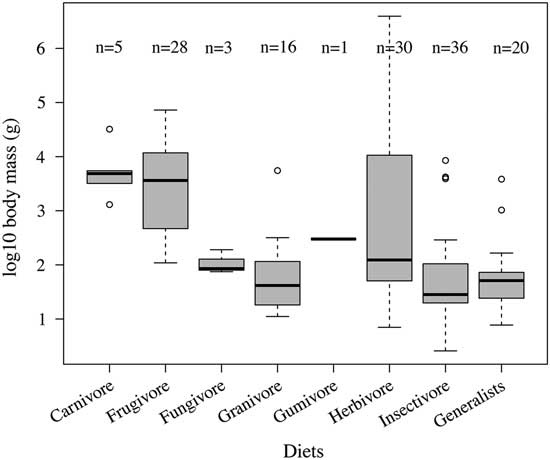
Figure 1 Box plot illustrating the body-mass range for each dietary category of the 139 mammal species in the data set. Categories are as described by Pineda-Munoz and Alroy (Reference Pineda-Munoz and Alroy2014).
Table 1 p-Values of pairwise comparisons based on the Wilcoxon rank-sum test for body-mass distributions in diet categories as described by Pineda-Munoz and Alroy (Reference Pineda-Munoz and Alroy2014) for (A) the whole data set and (B) only rodents.

Table 2 Proportion of animals in each dietary category for each body-mass range as discussed in the text.

The first four components of the PCA together express 65.76% of the variance and correspond to five major groups of feeding resources: green plants, fruit, seeds, invertebrates, and vertebrates (Supplementary Table 4). The first component (19.4% of the variance) mainly discriminates between a group of small-sized mammals that feed on invertebrates or roots and tubers, to the left of the chart, and the ones mainly feeding on green plants, to the right of the chart (Fig. 2). The second component (17.53% of the variance) discriminates mainly between medium-sized fruit eaters in the bottom of the chart and seed eaters on the top right of the chart (Fig. 2). Therefore, the two first components alone identify the four major feeding groups. The third component (15.19%) discriminates between many of the food resources, with especially high values for fungus and flower–gum eaters. The vertebrate-feeding variable loads strongly only on the fourth component (13.64% of the variance). Some degree of overlap can be observed between the groupings (Fig. 2), which could be related to the amount of food mixing displayed by some species. For example, many of the species in our data set mix seeds and vegetation in their diet. The same patterns can be observed in the data from Wilman et al. (Reference Wilman, Belmaker, Simpson, de la Rosa, Rivadeneira and Jetz2014) (see Supplementary Table 5 and Supplementary Fig. 3).
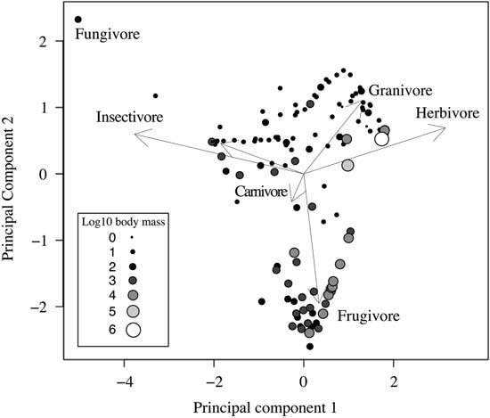
Figure 2 Scores of the two first axes of the PCA of dietary data for all the 139 species in the data set (adapted from Pineda-Munoz and Alroy [Reference Pineda-Munoz and Alroy2014]). Raw data are percentage of stomach content examinations rescaled to z-scores. Arrows indicate loadings on the two first components. Sizes indicate the log10 body mass (g) of each species as shown in the legend.
Figure 3 shows that species with extreme body sizes (micro- and megamammals) have more specialized and less diverse diets on average as based on the inverse Simpson index (Table 3). Micromammals (<10 g) are represented by three lipotyphlans with pure insectivore diets and two rodents having herbivore and generalist diets. Small mammals (10–999 g) display the most diverse diets (Fig. 3 and Table 3). They mostly belong to two taxonomic orders: Rodentia (75%) and Lipotyphla (10.9%). Medium-sized mammals (1–30 kg) mainly have frugivorous (51.5%), herbivorous (15.1%), carnivorous (12.1%), or insectivorous (12.1%) diets, and they mainly belong to the orders Primates (36.4%), Carnivora (30.3%), and Artiodactyla (18.2%). Large mammals (>30 kg) are only represented by six artiodactylan species, two carnivorans (Ursus arctos and Canis lupus), and a proboscidean (Loxodonta africana). The same patterns are seen in the data from Wilman et al. (Reference Wilman, Belmaker, Simpson, de la Rosa, Rivadeneira and Jetz2014) (see Supplementary Fig. 4).

Figure 3 Relationship between log10 body mass (g) and diet diversity indices calculated by applying inverse Simpson indices to stomach content percentages. Colors and shapes represent different dietary specializations as shown in the legend. The line connects the maximum dietary diversity value for each half-log10 unit to allow visualization of the maximum degree of food mixing. Ursus arctos has been excluded from the maximum dietary diversity curve to allow better visualization of the general pattern and for reasons mentioned in the text.
Table 3 Average, standard deviation, and maximum diet diversity values for each body-mass range as discussed in the text.

Around 50% of the medium-sized mammals in our data set have a frugivorous diet, and 75% of the frugivorous species fit in the medium-size range. We also found that 46.6% of the geographical distributions of the pure frugivores and 54.6% of the distributions of the mixed frugivores (Fig. 4) overlap with the distribution of tropical and subtropical moist broadleaf forests as defined by Olson et al. (Reference Olson, Dinerstein, Wikramanayake, Burgess, Powell, Underwood, D’amico, Itoua, Strand and Morrison2001). Some differences can be observed in the geographic distribution patterns between South America and Africa. While South American frugivores only occur within the tropical rain forest region, the ones in Africa show wider distributions, sometimes ranging into such biomes as tropical savannas.

Figure 4 Geographical distribution of tropical and subtropical moist broadleaf forests (adapted from Olson et al. [Reference Olson, Dinerstein, Wikramanayake, Burgess, Powell, Underwood, D’amico, Itoua, Strand and Morrison2001]) and of pure frugivore and mixed frugivore species in our data set (extracted from Map of Life [2016]).
Discussion
Body Mass and the Degree of Diet Specialization
Our results show how most dietary specializations are restricted to certain body-size classes in mammals. In a general way, this sort of pattern has been previously related to phylogenetic, ecological, and energetic constraints (Eisenberg Reference Eisenberg1981; Gittleman Reference Gittleman1985; Price and Hopkins Reference Price and Hopkins2015). Smaller mammals in our data set, having higher daily energy and protein requirements, generally require highly digestible food resources (i.e., grains, fungi, and insects; Clauss et al. Reference Clauss, Steuer, Müller, Codron and Hummel2013). They require less dietary specialization, because these particular food resources are usually abundant enough to support large populations. Some small mammals also display an herbivorous diet, which has been suggested to be a consequence of ecological opportunity rather than being related to any physiological advantage (Clauss et al. Reference Clauss, Steuer, Müller, Codron and Hummel2013).
In contrast, large mammals are not able to forage on high-nutritive rapidly digestible foods, because these resources are too rare to support their populations. Instead, they specialize their feeding on vegetation, a much more abundant food resource. Our results support this idea and show how dietary diversity decreases with increased body mass as a general trend. Having lower requirements for energy and nutrients per unit of body weight allows large mammals to feed on less nutritive resources (i.e., structural plant material) and get most of their nutrients from a very specialized diet (Demment and Van Soest Reference Demment and Van Soest1985; Clauss et al. Reference Clauss, Schwarm, Ortmann, Streich and Hummel2007, Reference Clauss, Steuer, Müller, Codron and Hummel2013). Increased body size allows herbivores to evolve gut structures that increase volume and retention time of the ingesta, and so they are capable of extracting a higher fraction of nutrients from low-energetic plant materials (i.e., leaves and grasses). However, it has been observed that long retention times are not characteristic of very large mammals. In those cases, other ecological advantages such as larger home ranges, predator avoidance, or resource competition are a potential benefit of large body size (Clauss et al. Reference Clauss, Schwarm, Ortmann, Streich and Hummel2007, Reference Clauss, Steuer, Müller, Codron and Hummel2013; Steuer et al. Reference Steuer, Südekum, Tütken, Müller, Kaandorp, Bucher, Clauss and Hummel2014).
Most micromammals (<10g) in the data set display a rather specialized insectivorous diet. Their high metabolic costs require them to feed on food resources with substantial energy content such as insects (Peters Reference Peters1986). Additionally, their small size might mechanically restrict their diets to small invertebrates (Fisher and Dickman Reference Fisher and Dickman1993). Thus, it could be postulated that extreme body sizes require higher levels of specialization and that the optimum for a very diverse diet must lie in the small range (10–999 g) (Raia et al. Reference Raia, Carotenuto, Passaro, Fulgione and Fortelius2012), as it does.
Among predators (pure insectivores and carnivores), the maximum body mass for the insectivores in our data set is 8.5 kg, with larger predators being carnivores. Similarly, Carbone et al. (Reference Carbone, Mace, Roberts and Macdonald1999) estimated a maximum sustainable mass of 21.5 kg for invertebrate diets, although some exceptionally larger insectivore mammals such as the aardvark (Orycteropus afer, 52 kg) do exist. Additionally, the average size of the pure insectivore mammals in Wilman et al. (Reference Wilman, Belmaker, Simpson, de la Rosa, Rivadeneira and Jetz2014)—the biggest data set known so far—is 914 g. Previous research suggested that myrmecophagous mammals from Afrotropical forests seemed to have the lowest population densities. Thus, resource availability might be limiting the maximum body mass of insectivores.
As mentioned, the maximum degree of food mixing tends to decrease with increasing body mass. However, the brown bear U. arctos falls outside this pattern according to the dietary diversity statistic. Surviving hibernation requires storing energy by consuming highly energetic food resources and increasing body fat (Humphries et al. Reference Humphries, Thomas and Kramer2003). In early spring, when more energetic and protein-rich foods are less abundant, U. arctos feeds on vegetation. However, it switches to a more nutritious diet in late summer. This mixed diet would be beneficial for supporting a seasonal higher demand of nutrients before periods of hibernation (Beeman and Pelton Reference Beeman and Pelton1980; McLellan Reference McLellan2011). Thus, U. arctos and other generalist hibernating ursids feed on a diverse, unspecialized diet despite their high body mass.
A few of the generalist species in the data set show a less diverse diet than some classified as specialists, which could be explained as a mathematical artifact arising in unusual circumstances. For example, an animal feeding on 60% vegetation, 10% insects, 10% fruit, 10% fungi, and 10% seeds would be classified as an herbivore, but its diet will be more diverse (inverse Simpson index = 1.23) than that of an animal eating 45% vegetation, 45% fruit, and 10% fungi (inverse Simpson index = 0.95).
Frugivory and Body Mass
Most dietary specializations have an optimum body-mass range, and few dietary specializations occur in the medium-size range; the only common ones are herbivory, frugivory, and carnivory. Most frugivorous mammal species in our data set have a body mass between 500 g and 30 kg. Previous studies found similar patterns, suggesting a peak in frugivory in the medium-size range for Neotropical primates (Kay Reference Kay1984; Robinson and Redford Reference Robinson and Redford1986; Hawes and Peres Reference Hawes and Peres2014). A diet with a very high proportion of fruit has been proposed to constrain body size due to mechanical, locomotional, ecological, and metabolic factors (Milton and May Reference Milton and May1976; Robinson and Redford Reference Robinson and Redford1986; Hawes and Peres Reference Hawes and Peres2014).
Hawes and Peres (Reference Hawes and Peres2014) performed an exhaustive study on the frugivory of Neotropical primates with special attention paid to the relationship with body mass. They observed higher rates of frugivory in medium-sized primate species (2–3 kg). The proportion of fruit in the diet of smaller species was much lower, with a higher intake of seeds and insects, while the largest ones foraged on an increasingly higher amount of foliage, a pattern also observed in previous studies (Kay Reference Kay1984).
Frugivore species in our data set are distributed around tropical and subtropical moist broadleaf forests. Thus, species with a higher percentage of fruit in their diet have a more restricted geographical distribution. They can also be found in forested patches in the surrounding areas, where they have to complement their diets with other food resources such as vegetation or insects, as shown in our resource utilization data set (see Supplementary Table 1).
We recorded frugivore species in tropical environments in South America and Africa but not in Southeast Asia and the Indo-Pacific (Fig. 4). This fact could be related to the nature of our dietary data. Pineda-Munoz and Alroy (Reference Pineda-Munoz and Alroy2014) limited their study to the stomach content literature in order to standardize data and avoid sampling bias. Unfortunately, very little stomach content research has been performed in the latter two regions. However, there are some examples of medium-sized tropical frugivores in these regions, such as the Indian giant squirrel Ratufa indica, with an average adult size of 1.5–2 kg; the liontail macaque Macaca silenus, with an average size of 3–10 kg (Ganesh and Davidar Reference Ganesh and Davidar1999); and the binturong Arctictis binturong, with an average size of 9–20 kg (Colon and Campos-Arceiz Reference Colon and Campos-Arceiz2013).
Similarly, the more restricted geographical distribution of South American frugivore species as compared with African ones could be related to sampling biases and a higher level of endemism in the South American region. Stomach content studies have been mainly carried out near the Amazon River. However, South America seems to have a high diversity of frugivore species such as primates, which ultimately results in allopatric, closely related species having more restricted geographic distributions (Wilson et al. Reference Wilson1988). Pure frugivores such as the black uacari (Cacajao melanocephalus) or the Colombian woolly monkey (Lagothrix lugens) can be found in areas surrounding those that provided most of the South American stomach content data.
We hypothesize that a wholly frugivorous diet is only suitable in tropical rain forests or similar biomes, where fruit resources are available all year round. Seasonality of precipitation or outright aridity prevents species from specializing on an entirely frugivorous diet in more open environments (Ganesh and Davidar Reference Ganesh and Davidar1999). Thus, based on our results we predict that medium-sized mammals should be less frequent in open environments. These observations are consistent with Rodríguez (Reference Rodríguez1999), who quantitatively documented a decrease in the density of mid-sized mammals in increasingly open landscapes.
Plant species composition in open environments is highly heterogeneous, with fruiting trees widely dispersed across space. As a consequence, frugivores in such environments would have to rely on a food resource that is rather unstable and patchily distributed, which would therefore require them to have unrealistically large home ranges (Milton and May Reference Milton and May1976; Ganesh and Davidar Reference Ganesh and Davidar1999).
According to optimal foraging theory, diet choice is conditioned by the need to maximize energy intake per unit of time spent on the foraging activity (MacArthur and Pianka Reference MacArthur and Pianka1966; Bartumeus and Catalan Reference Bartumeus and Catalan2009). An animal relying on a patchily distributed resource will then be forced to face a trade-off between the nature of resources and the energy required to move from patch to patch (Pyke et al. Reference Pyke, Pulliam and Charnov1977; Bartumeus and Catalan Reference Bartumeus and Catalan2009). Thus, the productivity and the species distribution of fruit trees in tropical rain forests play an important role in the evolution of the relationship between diet specialization and body mass in tropical mammalian species. This trade-off explains why the optimum body mass for a frugivore diet would fit around the medium-size range (1–30 kg). The energy invested in foraging activity—moving across patches or climbing trees—is cost ineffective for smaller and for bigger species (Pyke et al. Reference Pyke, Pulliam and Charnov1977; Bartumeus and Catalan Reference Bartumeus and Catalan2009). A pure frugivore diet is therefore restricted to the medium-size range within which foraging efficiency reaches its maximum.
Frugivory and the Medium-size Gap
Many ecological analyses have pointed out the decline or absence of medium-sized mammals (500 g–30 kg) in open-environment mammalian communities. Some interpretations in the literature include predator–prey relationships; trophic, physiological; and mechanical constraints; taxonomic limitations; or predator avoidance (Valverde Reference Valverde1967; Legendre Reference Legendre1986; Gingerich Reference Gingerich1989; Smith and Lyons Reference Smith and Lyons2011).
Alroy et al. (Reference Alroy, Koch and Zachos2000) hypothesized that the opening of a medium-size gap in North America during the middle of the Cenozoic could be linked to increased seasonality. The mid-size range was emptied during the middle Eocene (about 46 Ma) as ecosystems became more arid and seasonal. Alroy and colleagues also recognized a decrease in ecomorphological diversity after this period, as arboreal frugivorous species were replaced by large terrestrial herbivores. This interpretation supports our idea of a relationship between the opening of a medium-size gap and the decrease or disappearance of frugivore species in open environments.
Additionally, Alroy (Reference Alroy1998) recognized a general evolutionary trend in North American mammals toward increased body mass during the Cenozoic. However, he observed an upper size limit to the evolution of small taxa around 500 g, where the mid-size gap starts in North American mammals. This limit would have been established when vegetation structure changed toward more open landscapes, reducing the number of niches left to explore. In parallel, medium-sized tree-dwelling mammals evolved toward increased body size (Alroy Reference Alroy1998) or were replaced by open-environment herbivores. Interestingly, and as pointed out by Smith and Lyons (Reference Smith and Lyons2011), the upper limit of the mid-size gap coincides approximately with the lower limit observed for ruminant herbivores (5–10 kg) (Demment and Van Soest Reference Demment and Van Soest1985).
The Consequences of Improper Diet Classifications
All paleoecological methods make assumptions. In particular, biological parameters need to be categorized properly in order to statistically test their relationships with ecological and climatological variables. The present results suggest that the dietary categories of Pineda-Munoz and Alroy (Reference Pineda-Munoz and Alroy2014) strongly correlate with body mass, which suggests that the classification is useful. Additionally, recent research has shown that this classification correlates well with dental morphology (Pineda-Munoz 2015).
Fernández-Hernández et al. (Reference Fernández-Hernández, Alberdi, Azanza, Montoya, Morales, Nieto and Peláez-Campomanes2006) statistically tested some paleoecological methods—ecological diversity analysis (Andrews et al. Reference Andrews, Lord and Evans1979) and cenograms (Legendre Reference Legendre1986)—to evaluate their power as climate and paleoclimate estimators. The significance of the individual paleoecological variables used in these methodologies was also examined. The variables were taxonomic affiliation, trophic relationship, locomotion, and body size. The results suggested that body size was the best ecological variable, of those tested, for inferring climate. However, the dietary classification was statistically untested and ambiguous, because frugivorous and granivorous species were put together in a single category. Our data set shows that frugivore and granivore mammals have statistically different body-size ranges (p < 0.05; see Table 1). Thus, including them in a single category masked some ecological signals, which may have caused diet to be undervalued as a climatological indicator (Fernández-Hernández et al. Reference Fernández-Hernández, Alberdi, Azanza, Montoya, Morales, Nieto and Peláez-Campomanes2006). Furthermore, the geographical distribution of the frugivorous species in our data set shows a strong correlation between frugivory and tropical and subtropical climates. Thus, if frugivores had been separated from granivores, diet would have better discriminated between rain forests and open savannas. This observation reinforces the idea that a more comprehensive dietary categorization can more greatly empower paleoecology.
Acknowledgments
We thank M. McCurry and Xuan Zhu for assistance with GIS analysis. We also thank Nick Chan, David M. Alba, colleagues at Macquarie University and National Museum of Natural History Smithsonian Institution, and two anonymous reviewers for comments and suggestions. S.P.-M. was supported by Macquarie University’s HDR Project Support Funds and a Peter Buck Predoctoral Research Fellowship from Smithsonian NMNH. A.E. acknowledges the support of the Australian Research Council and Monash University. This is the Evolution of Terrestrial Ecosystems Program publication number 339.
Supplementary Material
Supplemental materials deposited at Dryad:: doi:10.5061/dryad.br45b.


