


Introduction
The Archaeocyatha are an extinct group of aspiculate sponges (Fig. 1) that appear very early in the Cambrian, forming extensive reef communities (Wood Reference Wood1999; Debrenne Reference Debrenne2007; Gandin and Debrenne Reference Gandin and Debrenne2010; Debrenne et al. Reference Debrenne, Zhuravlev and Kruse2012; R Core Team 2018) and shortly after the first appearance of sponge fossils (Carrera and Botting Reference Carrera and Botting2008; Antcliffe Reference Antcliffe2013, Reference Antcliffe2015; Antcliffe et al. Reference Antcliffe, Callow and Brasier2014; Muscente et al. Reference Muscente, Michel, Dale and Xiao2015; Nettersheim et al. Reference Nettersheim, Brocks, Schwelm, Hope, Not, Lomas, Schmidt, Schiebel, Nowack, De Deckker, Pawlowski, Bowser, Bobrovskiy, Zonneveld, Kucera, Stuhr and Hallmann2019). While now widely recognized as an extinct class of Porifera (Debrenne et al. Reference Debrenne, Zhuravlev and Kruse2012; Antcliffe et al. Reference Antcliffe, Callow and Brasier2014), their taxonomic affinities were disputed until the 1990s (Debrenne and Vacelet Reference Debrenne and Vacelet1984; Kruse Reference Kruse1990; Rowland Reference Rowland2001). Given their abundance and global distribution, the archaeocyaths have become important index fossils for correlating rocks on a global scale, meaning that we have detailed knowledge of their taxonomy and systematics (Debrenne et al. Reference Debrenne, Zhuravlev and Kruse2012; Gradstein et al. Reference Gradstein, Ogg, Schmitz and Ogg2012). The Archaeocyatha are the first undoubted metazoans to form extensive reef-like bioconstructions in association with calcimicrobes (Brasier Reference Brasier1976; Rowland and Gangloff Reference Rowland and Gangloff1988; Gandin and Debrenne Reference Gandin and Debrenne2010), and they therefore play a pivotal role in early Cambrian ecology (Wood et al. Reference Wood, Zhuravlev and Debrenne1992; Wood Reference Wood1999; Zhuravlev et al. Reference Zhuravlev, Naimark and Wood2015; Cordie and Dornbos Reference Cordie and Dornbos2019). Studies on their functional morphology have been extensive and show the Archaeocyatha were suspension feeders (Wood et al. Reference Wood, Zhuravlev and Debrenne1992; Debrenne et al. Reference Debrenne, Zhuravlev and Kruse2012). The reef communities of archaeocyathan sponges meant many individuals lived in close proximity. Ordinarily such close assembly leads to increased competition for suspended food resources, particularly given that in the early Cambrian the global abundance of phytoplankton and zooplankton is thought to have been much lower than modern levels (Servais et al. Reference Servais, Owen, Harper, Kröger and Munnecke2010; Cordie et al. Reference Cordie, Dornbos, Marenco, Oji and Gonchigdorj2019). In modern animal communities, resource partitioning is a common strategy used to reduce food competition between coexisting taxa (Gili and Coma Reference Gili and Coma1998). However, it has long been known that modern sponge communities do not play by the same ecological rules as most metazoan communities (Reiswig Reference Reiswig1971; Wulff Reference Wulff2006). Modern sponges do not partition prey before ingestion, only during retention, meaning there is little competition between them for this resource (Reiswig Reference Reiswig1971). As a result, sponge-dominated communities are almost invariably not competition driven, but neutral associations (Reiswig Reference Reiswig1973). It seems that modern sponges are “different from all the other organisms for which the conceptual framework of ecology was developed” (Wulff Reference Wulff2006: p. 148). Sponge interactions, particularly in modern sponge-dominated communities, generally promote the “continued coexistence of all participating species” (Wulff Reference Wulff2012: p. 274). Such cooperation and passive association have not been observed for many Cambrian sponge communities formed by archaeocyaths (Zhuravlev et al. Reference Zhuravlev, Naimark and Wood2015). Rather, competitive interactions are well documented in Archaeocyaths, including characteristics such as overgrowth (bioimmuration), avoidance, and the secretion of aporous skeletal sheets to maintain barriers between individuals (Brasier Reference Brasier1976; Kruse Reference Kruse1990; Debrenne et al. Reference Debrenne, Zhuravlev and Kruse2012). Statistical analysis of extensive ecological data sets also indicate that archaeocyathan communities were selectively assembled (Zhuravlev et al. Reference Zhuravlev, Naimark and Wood2015), meaning that the individuals were competing to be present in the community. Archaeocyathan communities therefore behaved rather differently compared with modern sponge-dominated communities, and this seems to have been particularly true during the Tommotian (Cambrian Stage 2 in Siberia, Russia).
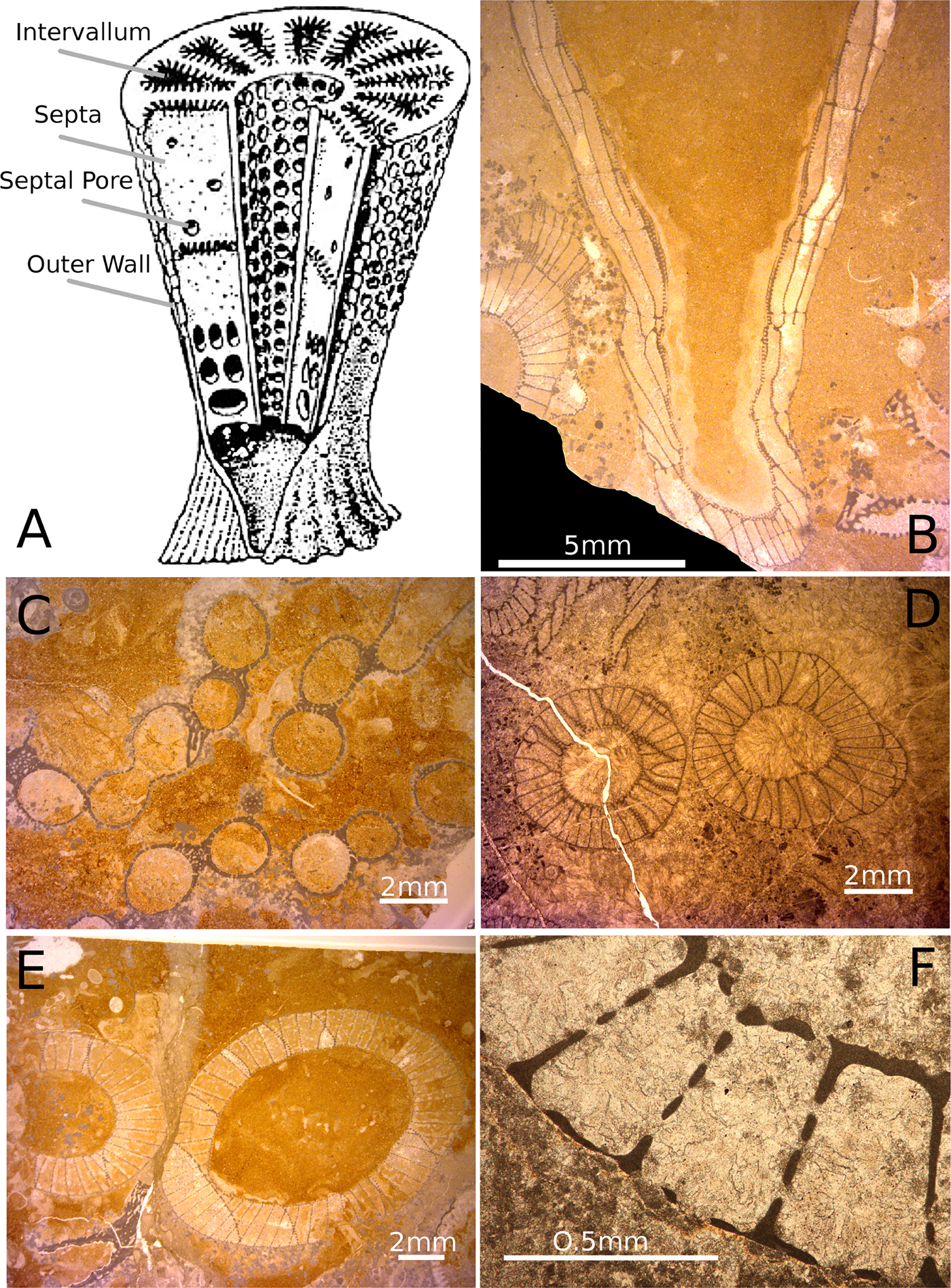
Figure 1. A, Schematic reconstruction of a double-walled archaeocyath showing the major characters discussed in the text. Adapted from a version in Antcliffe et al. (Reference Antcliffe, Callow and Brasier2014) from the original drawing of Debrenne et al. (Reference Debrenne, Zhuravlev and Rozanov1989). B–F, Archaeocyatha from the Siberian Platform in Russia, Terreneuvian to Cambrian Series 2 in age. B, A thin section of two archaeocyaths, central large specimen is in slightly oblique to longitudinal section, while the specimen in the bottom left is in transverse section. C, The archaeocyath Archaeolynthus polaris showing multiple modules. D, Two cups of an archaeocyath that show no growth avoidance and that are probably conspecific. E, Two cups of different archaeocyathan individuals showing growth avoidance. F, Close-up view of the two-walled structure of an archaeocyath showing the inner and outer walls, the septa, the intervallum space, and the inner-wall pores, outer-wall pores, and septal pores.
The structure of an archaeocyath skeleton (Fig. 1A,B) is thought to reflect the organization of the aquiferous system in life (Wood et al. Reference Wood, Zhuravlev and Debrenne1992). As suspension feeders, archaeocyaths filtered organic matter from the water column, which they brought into their body through pores or canals in their skeleton (Debrenne et al. Reference Debrenne, Zhuravlev and Kruse2012). Archaeocyaths had choanocytes (Debrenne et al. Reference Debrenne, Zhuravlev and Kruse2012) that would have helped generate a current drawing water from the outside of the sponge through the outer wall into the intervallum, the space between the inner and outer walls, and then out of the inner-wall pores to where it would have exited the cup (Balsam and Vogel Reference Balsam and Vogel1973). While some archaeocyaths were single walled (e.g., Archaeolynthus; Fig. 1C) most archaeocyaths had double walls (Fig. 1A,D–F), and the majority of living matter was located in the intervallum (the space between the two walls), and it would be here that phagocytosis of food would have taken place (Savarese Reference Savarese1992; Debrenne et al. Reference Debrenne, Zhuravlev and Kruse2012). The morphology of archaeocyaths is radically different from that of any living sponges, with the single genus Vaceletia being the only approximate morphological analogue, as the only surviving sphinctozoan sponge (Vacelet Reference Vacelet1977; Wörheide and Reitner Reference Wörheide, Reitner, Reitner, Neuweiler and Gunkel1996). Sphinctozoans are a polyphyletic grouping of similarly constructed sponges that reached their peak during the Permo-Triassic (Senowbari-Daryan and García-Bellido Reference Senowbari-Daryan, García-Bellido, Hooper, Van Soest and Willenz2002). There are many similarities between the polyphyletic sphinctozoan sponges and archaeocyaths, including the lack of spicules (e.g., in Vaceletia; see Vacelet Reference Vacelet1977), the massive calcareous skeleton, and the segmentation and partitioning of the skeleton (Kruse Reference Kruse1990). However, there are also fundamental differences such as the wall/pore elaborations in archaeocyaths, which are entirely absent in sphinctozoans. The wall microstructure is also different between archaeocyaths and sphinctozoan sponges, as is the stereoplasm, and the ontogenetic sequence of wall production, particularly in relation to the intervallum where food digestion takes place (Kruse Reference Kruse1990). Archaeocyaths are therefore unique in the evolutionary history of sponges and are morphologically distinct from all living sponges.
There has been little examination of what characters of the archaeocyaths were the primary focus for the observed competitive exclusions. According to ecology theory, the primary driving factors of competition are: resources (primarily food), the natural environment (e.g., space), and natural enemies (e.g., predators; Shea and Chesson Reference Shea and Chesson2002). As archaeocyaths had no known natural predators, and ecological studies suggest that they were often pioneer species so had little competition for local space (Zhuravlev et al. Reference Zhuravlev, Naimark and Wood2015), we here test the hypothesis that food was a limiting resource that drove competition in archaeocyathan communities. What archaeocyaths fed on is unknown, but is usually assumed to be bacteria, as these are important to the diet of extant sponges (Kruse et al. Reference Kruse, Zhuravlev and James1995; Debrenne and Zhuravlev Reference Debrenne and Zhuravlev1997). Modern sponges can feed on the whole size range of particles that can enter through their pores (ostia), albeit generally with reduced efficiency with increasing particle size (Leys and Eerkes-Medrano Reference Leys and Eerkes-Medrano2006). In archaeocyathan sponges, the size of the pores on the outer wall logically limited the size of food particles entering the skeleton, and when measured consistently, pore size can therefore provide an upper bound on the size of plankton that could have been phagocytosed by internal feeding cells. Archaeocyath outer-wall pore sizes, as well as septal and inner-wall pores (Fig. 1A,F), have been measured as a taxonomic indicator (Kruse Reference Kruse1982; Skorlotova Reference Skorlotova2013; Kruse and Moreno-Eiris Reference Kruse and Moreno-Eiris2014); however, pores have never been examined in an ecological context. Here we describe the feeding dynamics and prey partitioning of archaeocyathan reef communities by using measurements of the outer-wall pore diameter as a proxy for delimiting the size of suspended plankton entering the body and being consumed by the animal. Restrictive pore size data can also be used to examine the type of prey being consumed, because plankton fall broadly into distinct size categories that correlate well with biological grouping (Sieburth et al. Reference Sieburth, Smetacek and Lenz1978).
Materials and Methods
The archaeocyath material studied was derived from localities on the Siberian Platform in Russia (Fig. 2A) and is housed in the collections at the Muséum National d'Histoire Naturelle (MNHN) in Paris, France. The Siberian Platform consists of three major facies tracts of lower Cambrian, Nemakit–Daldynian to Toyonian in age, equivalent to Cambrian Series 1 (Terreneuvian) and Series 2, which displaced northeastward throughout the Cambrian (Khomentovskiy and Repina Reference Khomentovskiy and Repina1965). The fossil localities are now found where the Lena and Aldan Rivers intersect the archaeocyathan reef system. In general, there is a SW–NE trend of increasing paleo-water depth (Fig. 2A,B), with the archaeocyathan reef acting as a barrier between the shallow-marine, evaporitic, terrigenous system to the SW and the open fully marine deeper-water carbonates to the NE (Kruse et al. Reference Kruse, Zhuravlev and James1995). The specimens were predominantly collected during fieldwork by Peter D. Kruse, Andrey Yu. Zhuravlev, and Noel P. James (Kruse et al. Reference Kruse, Zhuravlev and James1995), from six localities in Siberia: Aldan, Byd'yangaya Creek, Churan, Zhurinskiy Mys’, Titirikteekh, and Oy-Muran (Fig. 2C). Archaeocyaths at these localities form meter-scale bioherms, where calcimicrobes such as Renalcis, living in association with the archaeocyaths were responsible for precipitating the majority of the calcium carbonate that comprises the bioherms (James and Debrenne Reference James and Debrenne1980; Gandin and Debrenne Reference Gandin and Debrenne2010). Taxa included in this study include the genera Nochoroicyathus, Coscinocyathus, Rotundocyathus, Erismacoscinus, and Tumuliolynthus (Fig. 3).
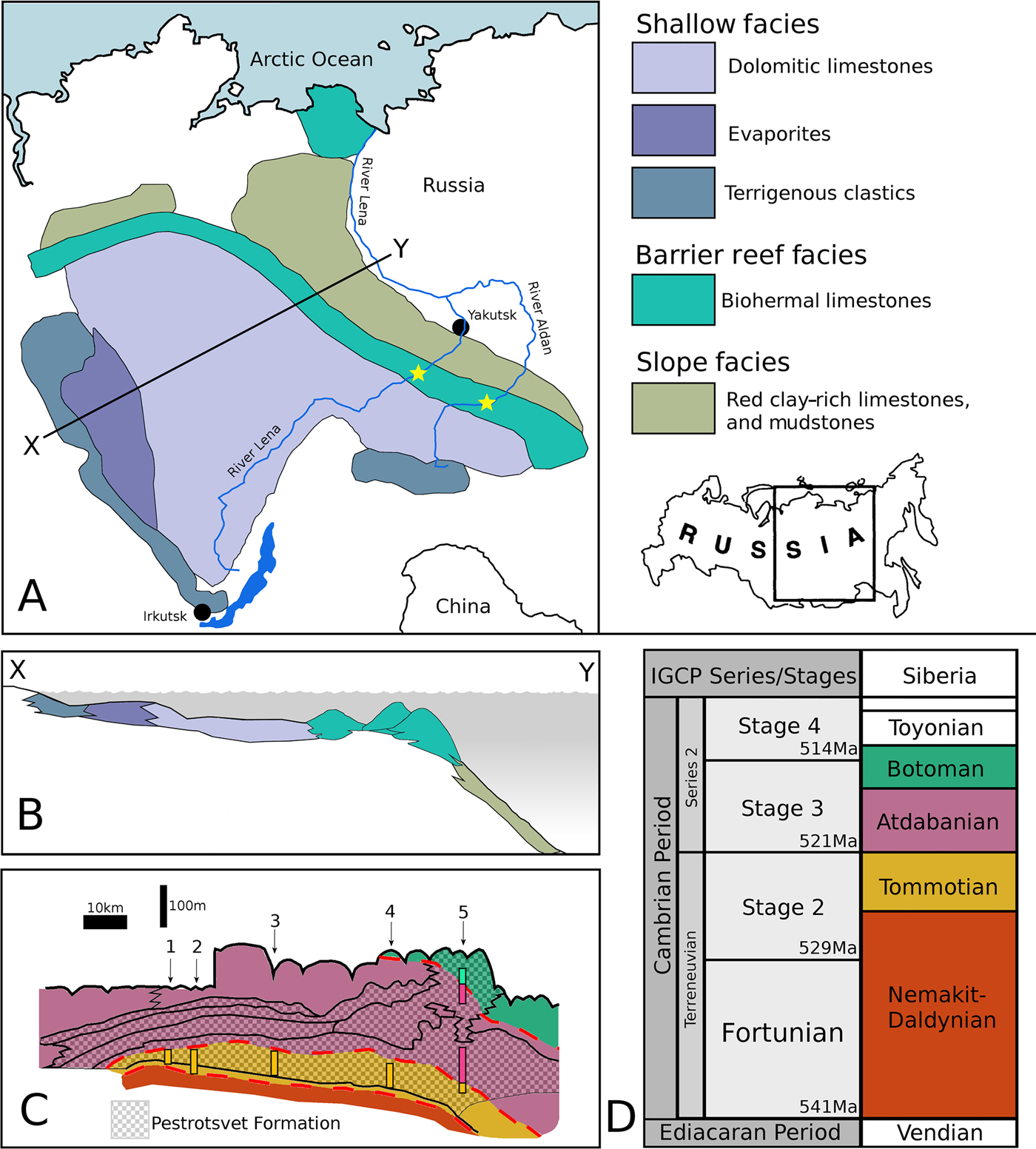
Figure 2. A, Map of the locality of the Siberian Platform in Russia, showing the extent of the platform with the three major facies tracts of Terreneuvian to Cambrian Series 2 in age. Stars show the position of the fossil localities on the Lena and Aldan Rivers from which the samples used in this study were taken. In general, there is a SW–NE trend of increasing paleo-water depth, with the archaeocyathan reef acting as a barrier between the shallow restricted marine system to the SW and the deeper marine system to the NE. Line X–Y denotes the line of section in part B. B, Schematic reconstruction of the facies relationships of the Siberian Cambrian. C, Schematic of a section along the River Lena, with the Pestrotsvet Formation crosshatched. Shadings (colors online) correspond to the timescale in D. Numbers indicate the positions of the localities discussed: 1. Titirikteekh; 2. Churan; 3. Byd'yangaya; 4. Zhurinskiy Mys’; 5. Oy-Muran. Highlighted bars show what age the specimens were drawn from for a particular section. After Kruse et al. (Reference Kruse, Zhuravlev and James1995). D, Timescale showing current best estimates for how the Siberian sections correlate with the global stage and series boundaries as recognized by the IGCP (Cambrian), compiled from Kruse et al. (Reference Kruse, Zhuravlev and James1995), Rozanov et al. (Reference Rozanov, Khomentovskiy, Shabanov, Karlova, Varlamov, Luchinina, Demidenko, Parkhaev, Korovnikov and Skorlotova2008), Gradstein et al. (Reference Gradstein, Ogg, Schmitz and Ogg2012), and Landing et al. (Reference Landing, Geyer, Brasier and Bowring2013).

Figure 3. Representative genera of Archaeocyatha from the Siberian fossil sites around the Lena River. All are from the collections in the Muséum National d'Histoire Naturelle in Paris. A,B, Nochoroicyathus; C, Coscinocyathus; D, Rotundocyathus; E, Erismacoscinus; F, Tumuliolynthus.
The global correlations of Cambrian strata are notoriously problematic, with only a few sections in the world (mainly Gondwana, e.g., Morocco and Australia, and Avalonia, e.g., the United Kingdom and Canada) providing any (even if very limited) absolute dates (Landing et al. Reference Landing, Geyer, Brasier and Bowring2013). The difficulties are then compounded by major facies differences between the different global sections, leading to extreme endemism of the fossils and making global biostratigraphy problematic and contentious (Landing et al. Reference Landing, Geyer, Brasier and Bowring2013). Most stratigraphic sections contain no lower Cambrian rocks (Peters and Gaines Reference Peters and Gaines2012). This time period coincided with one of the largest marine transgressions in Earth history, leading to subsequent extensive erosion and loss of lower Cambrian rock (Peters and Gaines Reference Peters and Gaines2012) as sea levels receded. As a result, lower Cambrian rocks are rare and difficult to correlate. Figure 2D compares the locally used stratigraphic terminology for Siberia with that of the globally correlated IGCP (International Geoscience Programme) series and stages. As these correlations remain to some extent problematic (Rozanov et al. Reference Rozanov, Khomentovskiy, Shabanov, Karlova, Varlamov, Luchinina, Demidenko, Parkhaev, Korovnikov and Skorlotova2008; Landing et al. Reference Landing, Geyer, Brasier and Bowring2013; Daley et al. Reference Daley, Antcliffe, Drage and Pates2018), the internally consistent Siberian terminology is adopted here, as that is how the material was catalogued in MNHN based on previous descriptions and the fieldwork collection data (Kruse et al. Reference Kruse, Zhuravlev and James1995).
The Oy-Muran material is difficult to date and was collected from two areas of distinct ages within the locality (Fig. 2). Consequently, they are separated in the analysis according to age: one is of latest Tommotian to Atdabanian (referred to as To-At Oy-Muran) and the other is dated between the Atdabanian and Botoman (At-Bo Oy-Muran). All the other localities are Tommotian in age. Within the Tommotian, Aldan is from the oldest strata; Churan, Titirikteekh, and Zhurinskiy Mys’ are all three derived from strata of a slightly younger age; and Byd'yangaya Creek is from the youngest strata (Kruse et al. Reference Kruse, Zhuravlev and James1995). They were also separated spatially, with each locality representing an area of exposed strata spaced several kilometers apart (Kruse et al. Reference Kruse, Zhuravlev and James1995) along the River Lena, while Aldan comes from sections on the River Aldan. (Fig. 2A,C).
Measurements of archaeocyaths were taken from rock thin sections mounted on glass slides. Any individual archaeocyath is referred to as a specimen, such that there may be multiple specimens on each thin section. The specimens from which measurements could be taken were identified to a genus level on each thin section by previous researchers, and when unclear, they were identified with help from A. Kerner (MNHN). A specimen was identified as suitable for use if it was possible to take at least five representative outer-wall pore measurements, although usually around 10 measurements were taken from each specimen. Pores had to be well enough preserved that the area within and around a pore could be distinguished clearly. Each thin section examined was digitally scanned, and the specimens to be measured were assigned labels (Supplementary Material). A Heidenhain Quadra-Chek with a Nikon Measuring Microscope with a binocular head was used to take the measurements.
Archaeocyaths can be clonally modular, that is, constructed of more than one cup (Debrenne et al. Reference Debrenne, Zhuravlev and Kruse2012) and are one of the earliest animal groups to have become clonal (Landing et al. Reference Landing, Antcliffe, Geyer, Kouchinsky, Bowser and Andreas2018). In life, the archaeocyath would have branched when creating clonal modules, which in thin section is not immediately obvious, because the connection may not be visible in the plane of section. Thus, one individual might produce many cups, which could appear to be separate individuals in thin section. This could lead to pore sizes on cups from the same individual being counted twice as separate specimens. It is therefore necessary to be able to distinguish between cups of separate individuals in close proximity and cups of one modular individual (Fig. 1C–E). Several indicators were used to distinguish modular forms from separate individuals, including the presence of immune responses (Brasier Reference Brasier1976) to dismiss the possibility of two or more morphologically similar archaeocyaths in close proximity being one modular form. Most of the archaeocyath species examined in this study were not modular, as modularity was rare in the Tommotian (Wood et al. Reference Wood, Zhuravlev and Debrenne1992).
Two different procedures were developed for measuring restrictive pore size depending on whether the section through the pore was transverse or longitudinal (Fig. 4). If a pore was cut at an angle that departed from either the longitudinal cut or the transverse cut, measurements were not taken, as neither technique would be appropriate (Figs. 4 and 5A,B). This often meant entire specimens were rejected, as all the pores were oblique cuts. To ensure the accuracy of the measurement from the information that can be gained from one view, each specimen was compared with different cuts of congeneric specimens. Previous studies measured outer-wall pore sizes (Kruse Reference Kruse1982; Skorlotova Reference Skorlotova2013; Kruse and Moreno-Eiris Reference Kruse and Moreno-Eiris2014) but did not take into account the commonly present features of pores that would have restricted the size of plankton that could pass through those pores. Such features include bracts (Fig. 5C), tumuli (Fig. 5D), and microporous sheaths. All of these features would have limited the size of particles that could pass into the archaeocyath. When such structures were present in the studied material, measurements were taken of the unobstructed gap left open by the additional feature. Broken walls were disregarded so as not to overestimate pore sizes (Fig. 5E). When both types of view were available on the same specimen, measurements were taken from both for later comparison (Fig. 5F). Having both longitudinal and transverse sections provides a complementary view of the pores to gain maximum information about the shape and structure of the pore.
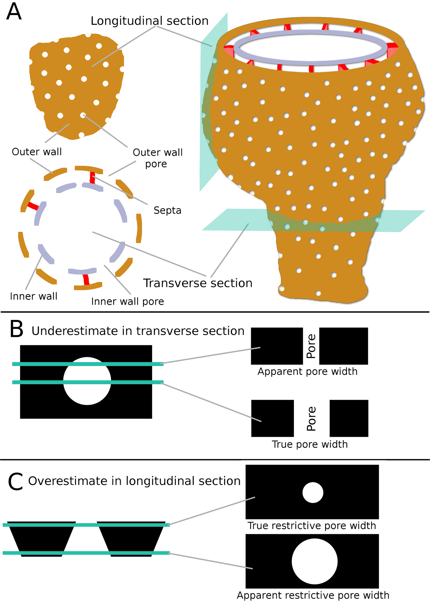
Figure 4. A, Schematic reconstruction of a typical archaeocyath showing the relationship of the major anatomical features to both longitudinal and transverse sections. B, Schematic drawing showing how pores in transverse section could appear smaller than the true diameter, if the section passes through anywhere other than the exact center of the pore. C, Schematic showing how pores in longitudinal view could appear larger than the true restrictive width, depending on the location of the section.
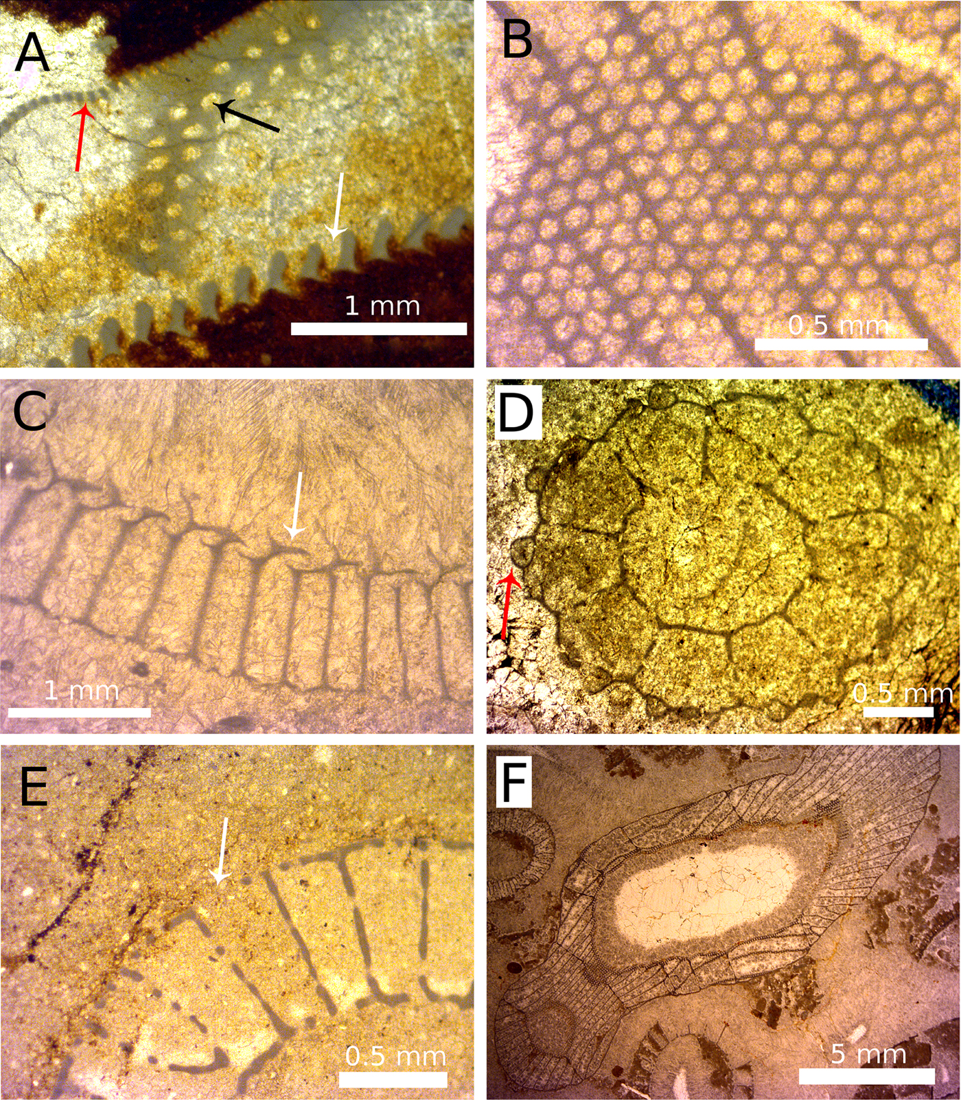
Figure 5. A range of features associated with pores and apparent restrictive pore widths. A, the three major pore types: dark gray (red online) arrow, outer-wall pore; black arrow, septal pore; white arrow, inner-wall canal. B, Varying pore sizes seen in slightly oblique section, with pores becoming more elliptical (to subpolygonal) to the right side of the image. C, Annuli are plate-like features (white arrow) that restrict the pore width and may add spiny and ornate coverings to the pore. D, Tumuli are sphere-like coverings (dark gray [red online] arrow) over pores that have one or more openings to allow transit of particles. E, An example of a broken outer wall (white arrow), producing a space in the wall much larger than the original pore. F, The irregular growth of archaeocyaths (e.g., if the specimens turns through 90° during growth) means that a single section can intersect the specimen in such a way that transverse, oblique, and longitudinal sections can be seen in a single specimen in thin section.
Measuring Outer-Wall Pore Diameter in Transverse View
A transverse view of an archaeocyath pore intersects the pore in a plane perpendicular to the surface of the outer wall. In thin section, pores in transverse view are visible along their entire depth from the exterior surface to the interior surface of the outer wall (Fig. 4C, right). In some specimens, the pore is parallel sided; alternatively, the pore diameter can narrow (be funnel shaped) along its length (Debrenne et al. Reference Debrenne, Zhuravlev and Kruse2012). In the case of a funnel-shaped pore, the restrictive pore size is the narrowest end of the pore. A transverse cut through a pore might make pore size appear smaller than it actually is if the cross-section does not cut through the pore at its maximum width (Fig. 4B, top right). Thus, thin sections of archaeocyaths can be misleading (McKee Reference McKee1963). To resolve this problem, measurements of restrictive pore size were only taken from the apparently largest pores on a specimen, as is the convention used by studies that measure other aspects of pore sizes (Kruse Reference Kruse1982; Skorlotova Reference Skorlotova2013; Kruse and Moreno-Eiris Reference Kruse and Moreno-Eiris2014). So in transverse view, restrictive pore size comes from the largest pores visible in section.
Measuring Outer-Wall Pore Diameter in Longitudinal View
Longitudinal views of pores intersect pores in a plane parallel to the outer-wall surface, such that the pores appear as circles in thin section. Incidentally, a longitudinal view of a pore will usually intersect the archaeocyathan cup slightly obliquely as the tangent to the cup wall, so a longitudinal cup view and a longitudinal pore view do not have to be the same, unless the wall is parallel to the cup axis. Longitudinal pore views only show the diameter of the pore at one point along its whole depth, and it can be unclear whether this is the narrowest point, potentially leading to overestimation of the restrictive pore size (Fig. 4C, right). To resolve this, only the pores that appeared smallest were measured. This approach also resolved problems connected to the presence of any features associated with more complex pores. For example, if the pores had bracts, the gap between the bract and the pore wall (the restrictive pore size) would appear smallest on the thin section. A few species of archaeocyaths have two distinct pore sizes, with one being noticeably smaller than the other. In these instances, the smallest pores among the distinctly bigger pores were measured. It should be noted that specimens with two distinct pore sizes would not affect the transverse view method, as the smaller pore type would be treated as an artifact and dismissed, because the largest visible pore diameter is measured in transverse view. Longitudinal views of pores often appeared noncircular. There are two reasons for this. First, if circular pores were cut at a slightly oblique angle, then pores would appear oval shaped (McKee Reference McKee1963). This is an artifact, and the true restrictive diameter can still be measured from the shortest dimension. Second, some archaeocyath species have true noncircular pores, although this was the case for only one taxon measured in this study. For noncircular pores, only the shortest distance was measured (the minor axis of the ellipse), as ingestion was still limited by the shortest distance across the pore.
Analyses
Data collected were input into Microsoft Office Excel and used to calculate mean outer-wall pore size, standard deviation, and coefficient of variance for each specimen. The statistical program R (R Core Team 2018) was used, specifically the packages arm for correlation and regression analyses and ggplot2 for plotting the figures. PAST (Hammer and Harper Reference Hammer and Harper2008) was used for Kolmogorov-Smirnov tests for examining data distribution. Pearson's was used for all correlations unless otherwise stated. All results are reported as three significant figures, unless an exact result was obtained. The results are split into four parts, the first two of which aim to test the validity of the methods. The second two aim to investigate aspects of archaeocyath feeding ecology. The method of analysis for each of these categories is described in the following sections.
Analyses of Transverse and Longitudinal Measurements from the Same Specimens
The aim of these tests was to determine whether the method used on longitudinal pores was measuring the same diameter as the method used to measure transverse pores. All the data for specimens across all the localities for which both longitudinal and transverse measurements had been taken were compiled, and mean pore sizes of each specimen were calculated for pores measured from the transverse and longitudinal sections separately. The two mean pore sizes were examined with linear regression, with a paired t-test performed for the support of regression gradient. The null hypothesis of these tests is that there are no significant differences between the mean pore sizes measured from transverse and longitudinal sections. As neither the transverse nor the longitudinal measurements can be designated as the dependent or independent variable, two linear regressions were carried out (x on y and y on x). One was for the transverse measurement against the longitudinal measurements. This makes transverse measurements the dependent variable, and so all the error is attributed to the transverse measurements. The other regression made longitudinal measurements the dependent variable so that the situation was reversed. The standard deviations and coefficients of variance of the measurements were also compared between the transverse and longitudinal data sets using t-tests and linear correlation to compare the dispersion of the measurements. The aim of these tests was to investigate whether there was equal variability in the longitudinal and transverse measurements from each individual specimen.
Analyses of Transverse and Longitudinal Measurements when Only One Type of Outer-Wall Pore View Was Taken per Specimen
Mean pore size data were collated for specimens in which pores in only one view had been measured. Although all the mean pore sizes of transverse measurements had been taken from different specimens than were used for the longitudinal measurements, it was reasoned that, for a locality, the transverse and longitudinal measurements should not be significantly different from each other, because the specimens for both theoretically represent a random sample of the same population. For this reason, the transverse and longitudinal measurements were only compared if they were from the same locality. Any significant differences in the overall mean of the mean pore sizes of transverse versus longitudinal measurements were tested using a Welch's t-test. A Welch's t-test was used as there would otherwise have been a slight violation in the assumption of constant variance. Data were subjected to a Box-Cox transformation to improve normality. These tests were used to investigate whether the mean pore size distribution for a locality as calculated from specimens for which only transverse measurements were taken was significantly different from the pore size distributions calculated from specimens from which only longitudinal measurements had been taken.
Comparisons of the Distribution of Mean Outer-Wall Pore Sizes between Localities
The aim of these tests was to test for any significant differences between the distribution of pore sizes found at the different localities. Comparisons were made of the distribution of pore sizes at each locality using a series of two-sample Kolmogorov-Smirnov tests, a test that does not make any assumptions about the distribution of the data. This test compares the overall distribution of two samples by comparing the maximum difference between their cumulative probability distributions (Hammer and Harper Reference Hammer and Harper2008). The test was carried out on every combination of localities. As 21 tests had been carried out in total, the Benjamini-Hochberg procedure was used to control the false discovery rate, for a false discovery rate of 5%.
Results
Analyses of Transverse and Longitudinal Measurements from the Same Specimens
Comparisons of the Mean Outer-Wall Pore Sizes
In total there were 76 specimens for which mean pore size was calculated using both transverse and longitudinal measurements. A two-tailed paired t-test between the overall mean pore sizes of the longitudinal and transverse measurements showed no significant difference (t(75) = 0.46, p-value = 0.640). This provides evidence that there is no systematic difference between the two methods. Results of the linear correlation analyses indicate that there is a highly significant correlation between the size of pores as measured by transverse and longitudinal mean pore size (r 2 = 0.930, F(1,74) = 946, p-value < 2.20 × 10⁻¹⁶).
An analysis of the correlation between transverse and longitudinal measurements was performed when these could be measured from the same specimen. The regression of longitudinal mean pore size on transverse mean pore size gave a slope of 0.95 and an intercept of 3.90. The regression of transverse mean pore size on longitudinal mean pore size gave a slope of 0.98 and an intercept of 0.85. The 95% confidence intervals (Table 1) for both regressions show that the intercept is not significantly different from 0 and the slope is not significantly different from 1 at the 95% confidence level, providing evidence that the two methods are measuring the same diameter. The lower bound for the gradient of the slope is 0.96 and the upper is 1.09, which still contains a slope of 1 (Fig. 6). The true relationship between the mean pore sizes as calculated by the two types of measurement would be expected to lie between these two lines with allowance for the small uncertainty of their confidence intervals. The correlation for longitudinal on transverse is excellent (r 2 = 0.938) and highly significant (p-value [slope] = 1.00 × 10−45). The results of these tests provide good evidence that the two types of measurement are measuring the same average pore diameter.
Table 1. The 95% confidence intervals for two linear regression analyses comparing outer-wall pore diameter measured from longitudinal and transverse sections.


Figure 6. Plot showing the correlation between outer-wall pore measurements in transverse and longitudinal section (n = 257 specimens).
Comparisons of Standard Deviation and Coefficient of Variance of Measurements used to Calculate Mean Outer-Wall Pore Size
The standard deviation was calculated for the measurements used to calculate mean pore size; there was a sample size of 70 SDs for transverse and longitudinal measurements. The two-tailed paired t-test gave an insignificant result (t (69) = 0.0441, p = 0.964). This indicates that the overall mean standard deviation for the transverse measurements is not significantly different from that of the longitudinal measurements. The correlation coefficient for the two variables was 0.570 (p-value = 1.97 × 10⁻⁷). This highly significant correlation suggests that the standard deviation of both transverse and longitudinal measurements increases as the other increases. To test this, the coefficient of variance was calculated for all the measurements for which standard deviation had been calculated. There was no correlation between the coefficient of variance for the transverse versus the longitudinal measurements (r 2 = 0.140, p-value = 0.235). These results support the hypothesis that the correlation in standard deviations was caused by the increase in mean pore size. Further, a paired t-test for the coefficient of variance also found no significant difference between the mean of the coefficient of variances for the two methods (t(69) = 0.345, p-value = 0.731). So neither method had a consistently higher coefficient of variance.
Transverse and Longitudinal Measurements when Only One Type of Outer-Wall Pore View Was Taken per Specimen
Box plots of the data (Fig. 7) show a trend of longitudinal measurements having lower medians and upper-quartile and lower-quartile values than transverse measurements. The longitudinal measurements also have a smaller interquartile range. Statistical tests were only carried out for data from At-Bo Oy-Muran and To-At Oy-Muran, because these sites had reasonably large and even sample sizes (26 for To-At Oy-Muran and 31 for At-Bo Oy-Muran; Fig. 7B). Welch's two-tailed t-tests were used on the transformed data for To-At Oy-Muran and At-Bo Oy-Muran. The result of the t-tests showed the means of the two types of measurements were significantly different from each other (t(23.2) = 3.0491, p-value = 0.00576 for To-At Oy-Muran and t(28.8) = 4.00, p-value = 0.000400 for At-Bo Oy-Muran). The 95% confidence intervals for the differences between the means showed that the mean longitudinal pore size (μL) was significantly less than the mean transverse pore size (μT) for both localities (−2.22 < μL − μT < −0.42 for To-At Oy-Muran; −2.61 < μL − μT < −0.85).
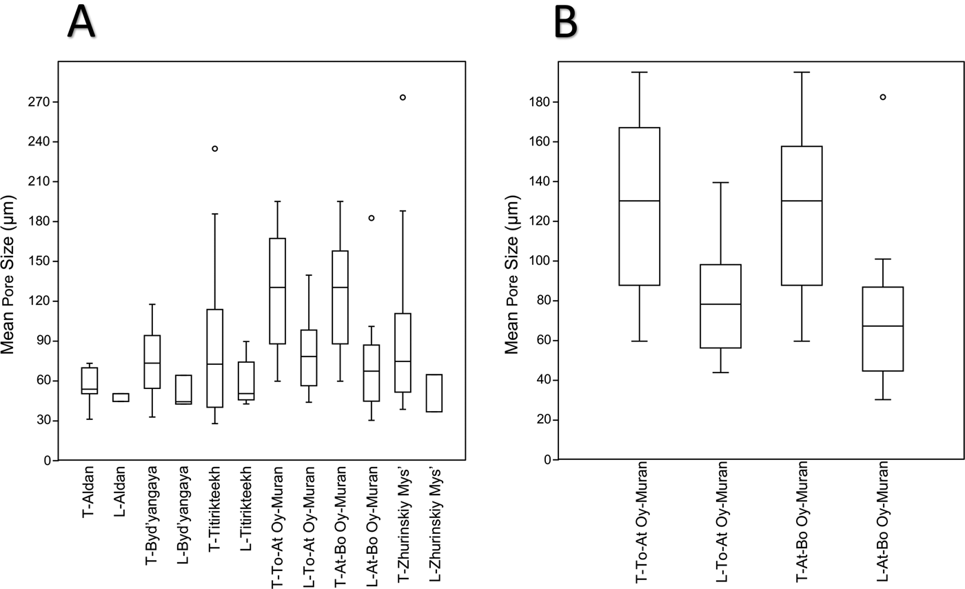
Figure 7. Box plots of outer-wall pore sizes measured separately for locality and section orientation. Any locality names with the prefix “T” are measurements from transverse sections, and those localities with prefix “L” are measurements from longitudinal sections. The horizontal lines in the boxes represent, in order from top to bottom, the upper quartile, the median, and the lower quartile. Whiskers show the minimum and maximum values, excluding outliers. Outliers were defined as being further than 1.5 times the height of the box away from the box and are signified by circles. A, Data from all locality studies. B, Enlarged box plots for the two Oy-Muran localities.
Summary Statistics of the Mean Outer-Wall Pore Sizes
In total, data were collected for 257 specimens. The mean pore size for all the localities’ data combined was 81.5 μm, and the median pore size was 68.8 μm. The data were positively skewed, so although the maximum pore size was 273 μm, there were proportionally fewer high values with 75% of the data below 101 μm (Fig. 8). The minimum size recorded was 25.2 μm.

Figure 8. Histogram showing the frequency of archaeocyath specimens with a mean outer-wall pore size falling within the given size classes (12 bars, 21 μm wide). The global median is 68.8 μm and the global mean is 81.5 μm. The data skew positive, with 75% of specimens having pores smaller than 101 μm. The smallest mean restrictive pore size found was 25 μm, while the largest was 273 μm.
Comparisons of the Distribution of Mean Outer-Wall Pore Sizes between Localities
The sample size of mean pore sizes calculated for each locality were: Aldan = 14, Byd'yangaya Creek = 54, Churan = 10, To-At Oy-Muran = 32, At-Bo Oy-Muran = 40, Titirikteekh = 71, and Zhurinskiy Mys’ = 35. The results for the two sample Kolmogorov-Smirnov tests are shown in the Table 2. A majority of the significant results involve Aldan, suggesting that the distribution at this locality is particularly distinct. Byd'yangaya Creek and To-At Oy-Muran also had significantly different distributions. Aldan and Byd'yangaya Creek have smaller mean and median pore sizes than other localities (Table 3), and To-At Oy-Muran contains relatively higher numbers of specimens with large mean pore sizes. The other localities generally have distributions between these extremes.
Table 2. Comparing the outer-wall pore distributions by locality. The p-values for each pair of localities are shown above the diagonal line of black boxes, with bold text indicating significant results at 95% confidence after the Benjamini-Hochberg procedure. Below the line are the D-values associated with the p-values. At-Bo, Atdabanian to Botoman; To-At, Tommotian to Atdabanian.

Table 3. Mean and median outer-wall pore sizes for the archaeocyaths measured at each locality. At-Bo, Atdabanian to Botoman; To-At, Tommotian to Atdabanian.

Discussion of Method Validity
Analyses of Transverse and Longitudinal Measurements from the Same Specimens
The results support the hypothesis that the two methods are measuring the same pore diameter and that both methods for taking measurements give a similar approximation of the mean pore size of a specimen. This supports the validity of measuring a specimen's pore size with one method when only one view is available. A consequence of studying fossil material from extinct organisms is the difficulty of investigating any further whether the mean pore size estimated by the two methods is in fact the true restrictive width. However, this uncertainty is minimized by the close agreement of the two methods, which were both logically devised to measure the pore diameter at the narrowest point. The methodology will allow for the rapid and reliable measurement of the restrictive pore size of specimens for which only one view is available.
There are two possible causes of the variability of the measurements used to calculate the mean pore size for each specimen. One is that the variation in measurement reflects true natural variation in the pore size of a specimen. The rest of the variation would be due to measurement error, which could be caused by inaccurately measuring the diameter at the narrowest point of the pore: this is thought to have had minor effect, as the equipment used was well calibrated and measured with high precision (calculated as being correct within 0.4–2 μm over the measurement range of 25–273 μm, thereby representing an error range of 0.7–1.6%). The other component of measurement error was the measuring of pores at a point that was not exactly the “true” narrowest point of the pore. As explained in the “Materials and Methods” section, this could lead to either under- or overestimation of pore size depending on the cut of the section; this is difficult to quantify but was controlled for through examination of pores from multiple orientations and comparative analysis of longitudinal and transverse cuts. The proportion of the variability attributable to these factors cannot be calculated from the data. Regardless of the cause, the results of the correlation and regression analysis suggest the impact of these factors on the study is relatively minor. Analyses suggested that standard deviation increased with mean pore size, and so the overall measurement error and/or natural variability within a specimen is thought to have increased with mean pore size: either of these explanations are plausible. The effect of the increase in the variation of measurements on mean pore size calculations was reduced, because the mean pore size for a specimen was based on measurements taken from multiple pores. The results showed no evidence of the variability in measurements being different for either method, so the measurement error is the same for both methods. This suggests that both methods are equally reliable for measuring pore size. On this basis neither method can be recommended over the other.
Analyses of Transverse and Longitudinal Measurements when Only One Type of Outer-Wall Pore View Was Taken per Specimen
The unexpected trend for longitudinal measurements to be lower than transverse measurements in specimens with only one type of pore cross section may be best explained by sampling bias. Longitudinal measurements may tend to be taken from specimens with smaller pore sizes, because large pores viewed in longitudinal section are more likely to appear incomplete, as you do not see a definite margin in this view, just a space in the wall, which when very large may be interpreted as dissolution or fracture of the wall. As a result, longitudinal measurements were less suitable for inclusion in the study. This bias would explain the significant result of the t-test. Until the causes of this trend are resolved, the effect it has on the data is unknown, although if the explanation suggested is correct, it is likely that specimens with larger pores will be underrepresented. The effect of this should be relatively small, because only 16.4% of the specimens had only longitudinal pores. If a bias is found for longitudinal measurements, future studies may consider not including them. There is no evidence at the moment to suggest that these biases were present, however.
The difference between the means of longitudinal and transverse pores could also reflect the measurement methods of the smallest of the minimum measures for longitudinally viewed pores and the largest of the minimum measures for transversely viewed pores. This is interesting, because when the data from specimens in which both pore types could be measured are taken together, no significant difference could be found. This suggests that the overestimation of the mean from transverse pores alone could be being balanced out by the underestimation of the mean from the longitudinal pores alone. However, it is worth noting that these measures are still based on real pores, and it is only the mean that is affected, not the overall maximum. By performing our subsequent analyses with the means of the data and not the upper range value of maximum diameter for estimating prey size, we are taking a conservative approach to prey size range, as a given archaeocyath may have had some larger pores than the mean pore size for the specimen.
Quantifying the Effect of Living Tissue on Restrictive Pore Size
The restrictive pore size in life would have been constricted by the presence of the living cells that cover the body of sponges. In the closest living modern analogue to archaeocyaths, Vaceletia, the thickness of live cells covering the body wall is estimated to be between 2 and 20 μm (Kruse Reference Kruse1990). This comports well with direct evidence from fossil archaeocyaths, which suggests that the cellular layer is of a similar scale (see Kruse Reference Kruse1990: Fig. 6). The outer-wall pore diameter is constricted, therefore, by 4 to 40 μm (see Figure 9A), as the pore has living tissue around the entire circumference and constricts both margins of the diameter. The effects of this constriction on the present analysis is, however, insignificant, as the error can be well constrained and becomes insignificant as the pores get larger (Figure 9B). This could suggest a potentially hugely significant error on the smallest of the specimens, as the minimum outer-wall pores were ca. 25 μm, thus, in extremis, the entire pore could be covered by living cells (max. 40 μm), rendering the pore useless for suspension feeding. This implies the smallest pores had a cellular covering toward the thinner range of the spectrum. The minimum cell coverage (4 μm) on the smallest outer-wall pores measured reduces our smallest pores to ca. 21 μm, making little difference when we are considering their likely prey. However, by the time we are considering the largest pores, the error is constrained between a negligible 1.45% (for 4 μm out of 273 μm) to a manageable 14.5% (40 μm out of 273 μm). Thus, when considering the maximum size of prey that could be consumed by the largest pores (273 μm) measured in our study, we can constrain these pores to between 233 and 269 μm when allowance is made for the cells covering the archaeocyath in life. These ranges are significant when one examines the size ranges of possible prey groups, as we consider in the following section.
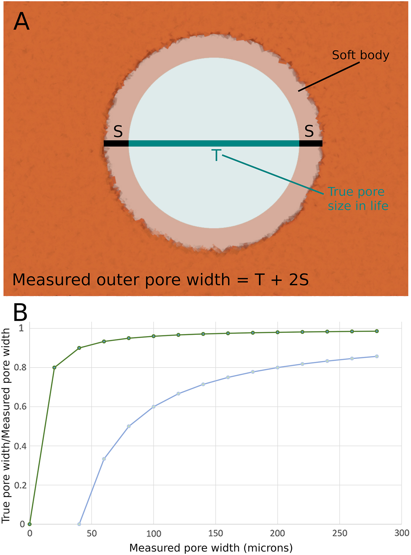
Figure 9. A, Schematic representation of the lining of the mineralized archaeocyath body wall with living cells. These cells would restrict the open pore size. B, Plot to show the percentile effects of the estimated cell thickness on the outer-wall pore diameter. The two curves show the maximum possible cell thickness (40 μm—lower curve, as it has a great effect on open pore diameter) and minimum possible cell thickness (4 μm—upper curve, as it has a lesser effect on open pore diameter).
Discussion of Implications for Cambrian Ecology
The data collected on outer-wall pore diameters provide information on the maximum size of plankton that could enter into the intervallum to be phagocytized by the archaeocyath. This study focused on only a few sites and a few genera, namely: Nochoroicyathus, Coscinocyathus, Rotundocyathus, Erismacoscinus, and Tumuliolynthus (Fig. 3). As archaeocyaths are a diverse group with a great deal of disparity in their skeletal morphology, these taxa do not represent the global range that could be found for archaeocyathan pores. It is therefore possible that the distribution of pore sizes could be different with a different sample of taxa, at different localities, and in different paleoenvironments. It is possible that other taxa could extend the range of pore sizes both upward and downward. Our conclusions are therefore conservative when considering total group Archaeocyatha.
How archaeocyaths fed has been the source of some debate. It has been suggested that archaeocyaths could possibly have housed symbiotic photoautotrophs that provided nutrition for the sponge (Wood Reference Wood1999; Debrenne Reference Debrenne2007). However, a photosymbiotic mode of life is now considered unlikely for a number of reasons. First, many archaeocyaths lived in areas of high sediment input, with high seston input, particularly of mud-sized particles (Kruse et al. Reference Kruse, Zhuravlev and James1995; Debrenne Reference Debrenne2007). As a result, light penetration would have been very poor, even in the most shallow-water environments that archaeocyaths inhabited; this would have made photosymbiosis unreliable and low yield. Second, carbon isotope data do not show the fractionations between archaeocyaths and marine cements that would be expected if the archaeocyaths were photosynthetic; this has been replicated at different sites in Australia (Surge et al. Reference Surge, Savarese, Dodd and Lohmann1997) and those sites in this study from Siberia (Brasier et al. Reference Brasier, Corfield, Derry, Rozanov and Zhuravlev1994). Finally, it has been argued that archaeocyaths predominantly lived in nutrient-rich environments, because they are often found co-occurring with fossil organisms with shells made with the bio-limiting nutrient phosphorous as an important component (Brasier Reference Brasier1991; Surge et al. Reference Surge, Savarese, Dodd and Lohmann1997). While such eutrophic conditions are very good for photosynthetic organisms, such as plants and free-living algae, it is very unusual to find animal–algal photosymbioses in such conditions, with modern reefal associations of this type strongly correlated with nutrient-poor conditions (Surge et al. Reference Surge, Savarese, Dodd and Lohmann1997; Gili and Coma Reference Gili and Coma1998; Kiessling Reference Kiessling2009). As a result, it is generally thought that bacterioplankton made up the main food resource for archaeocyaths (Wood et al. Reference Wood, Zhuravlev and Chimed-Tseren1993; Kruse et al. Reference Kruse, Zhuravlev and James1995; Debrenne and Zhuravlev Reference Debrenne and Zhuravlev1997). This is based on comparisons with studies of modern sponge ecology that show bacteria form a substantial part of many modern sponge diets (Reiswig Reference Reiswig1971; Leys and Eerkes-Medrano Reference Leys and Eerkes-Medrano2006), with bacterioplankton generally falling in the 0.2–2 μm range (see Fig. 10). Outer-wall pores in modern sponges are typically in the 30–60 μm range and can commonly reach 200 μm (Bergquist Reference Bergquist1978). However, the digestion of cells takes place in the aquiferous system in specialized choanocyte chambers. and the entrances to the choanocyte chambers are typically 5–10 μm (Bergquist Reference Bergquist1978; Bannister et al. Reference Bannister, Battershill and De Nys2012); thus, only particles smaller than 10 μm can be digested by most modern sponges. Particles between 10 and 100 μm can enter the sponge and travel through the aquiferous system but cannot enter the choanocyte chambers (Bannister et al. Reference Bannister, Battershill and De Nys2012), while particles larger than 100 μm have very little chance of entering the body of most modern sponges. The body size of archaeocyaths was significantly smaller on average than that of modern sponges (averages of 10.6 mm vs. 94.1 mm were found according to Cordie and Dornbos [2019]), yet our analysis indicates comparable outer-wall pore sizes in archaeocyaths and modern sponges. However, the internal morphology of archaeocyaths was quite unlike that of modern sponges. In archaeocyaths, digestion took place in the intervallum between the inner and outer wall—essentially this is equivalent of the choanocyte chambers in modern sponges. The entrance to the intervallum was through the outer-wall pores and there were no additional skeletal constrictions. The prey size and particle size were therefore not differentiated by the internal skeletal anatomy in archaeocyaths as they are in modern sponges. As pores in archaeocyaths are consistently two orders of magnitude larger than the size of bacteria, this could have made them susceptible to having to deal with higher levels of sediment input (Bell et al. Reference Bell, McGrath, Biggerstaff, Bates, Bennett, Marlow and Shaffer2015), which is highly problematic for sponges (Bannister et al. Reference Bannister, Battershill and De Nys2012), than would be necessary if archaeocyaths had much smaller pores. As a result, there needs to be consideration of whether larger plankton were an important part of the archaeocyath diet.
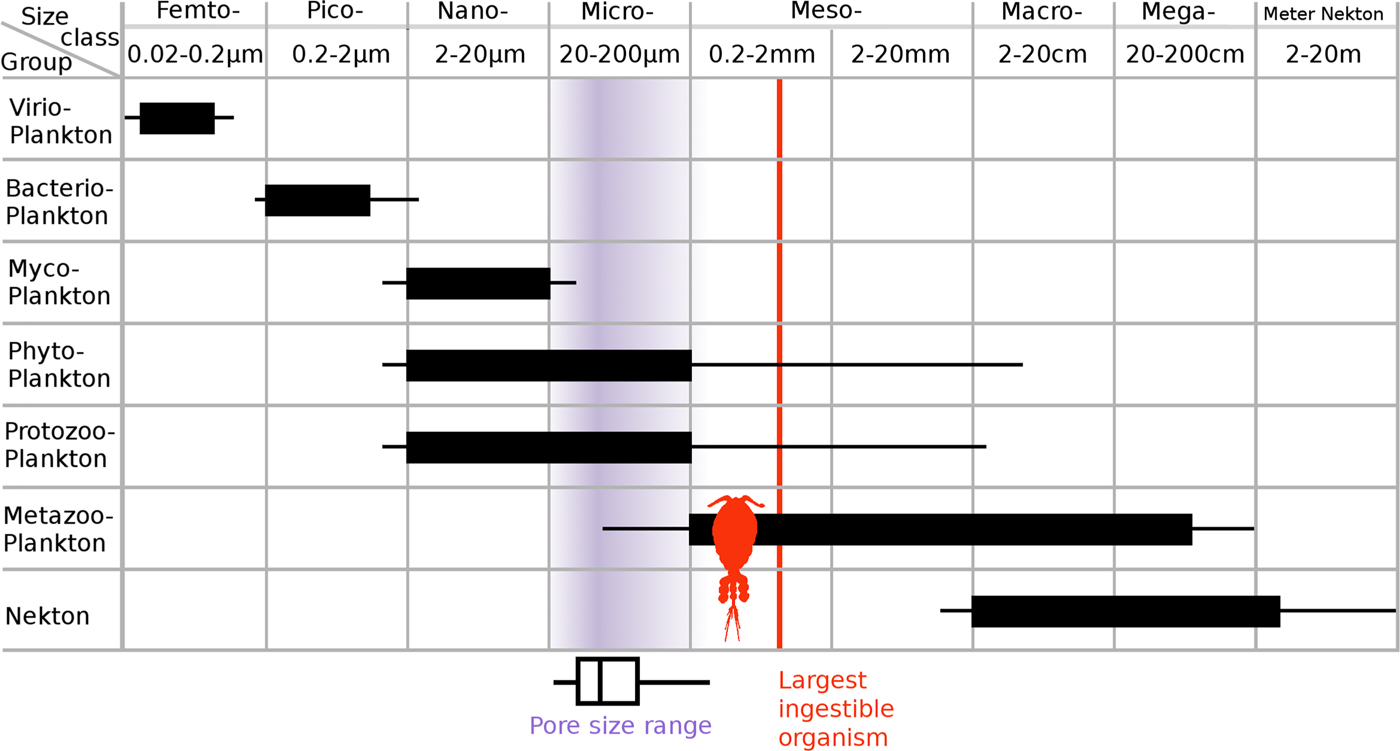
Figure 10. Relationship between the size classification of plankton and the biological function/phylogenetic class of plankton (after Sieburth and Smetacek Reference Sieburth, Smetacek and Lenz1978); note that horizontal scale is logarithmic. Phytoplankton consists of photosynthetic single-celled eukaryotic plankton and all autotrophic and mixotrophic single-celled eukaryotic plankton. Protozooplankton includes all single-celled heterotrophic eukaryotes, such as the ciliates and amoeboids. Metazooplankton includes all metazoan heterotrophic plankton and juvenile planktonic metazoans. The light gray (purple online) shading indicates the density of the data of archaeocyath mean pore sizes. The vertical line indicates the theoretical maximum length of plankton that could be consumed by the largest restrictive pores found in this study. Based on a typical 3:1 length to width ratio for copepods (Fernandez Araoz Reference Fernandez Araoz1991) and micro-current alignment of nonspherical prey items (Visser and Jonsson Reference Visser and Jonsson2000), a maximum prey body size would be 3 × 269 μm = 807 μm. Rather than simply being capable of eating bacterioplankton in the picoplankton range, even the smallest-pored archaeocyath would have been able to consume the nanoplankton range of the single-celled eukaryotic plankton groups, with several of the archaeocyaths being able to carnivorously consume micrometazoans.
Even considering the fact that pores may have been slightly restricted by living matter, all of the archaeocyath pores measured were well over 20 μm in diameter. This indicates that the whole size range of nanoplankton (2–20 μm) as well as a proportion of microplankton (20–200 μm) could easily enter the intervallum (Fig. 10; Sieburth et al. Reference Sieburth, Smetacek and Lenz1978; Omori and Ikeda Reference Omori and Ikeda1984). Generally, studies agree that phytoplankton in the nano- and microplankton size range form a significant part of the diet in most modern sponges (see review by Riisgård and Larsen Reference Riisgård and Larsen2010). These larger plankton (nano and micro) are believed to be taken up by cells such as the amoebocytes and collenocytes that line the inhalant passages (Conover Reference Conover and Longhurst1981; Riisgård and Larsen Reference Riisgård and Larsen2010). Plankton larger than 5 μm formed ~15% of the ingested carbon of the demosponge Dysidea avara, but a capacity for ingesting a broad range of food particles, particularly phytoplankton, was important for sustaining a constant food supply during winter when nutrient flux was lower (Ribes et al. Reference Ribes, Coma and Gili1999). These studies support the hypothesis that nanoplankton and microplankton may have formed an important part of the archaeocyath diet.
Nanoplankton and microplankton size classes can be produced by an array of different organisms (as can be seen from Fig. 10, following Sieburth et al. [1978]). Indeed, the 2–200 μm range is the only major class of plankton size that is commonly produced by a number different major types of organism (e.g., the picoplankton at 0.2–2 μm size range are produced almost exclusively by bacteria; the megaplankton at 20–200 cm are exclusively animal). Microplankton, however, are commonly produced by fungi (mycoplankton), photosynthetic eukaryotes (phytoplankton), and heterotrophic eukaryotes (protozooplankton). Using the restrictive pore size data to make predictions of which specific nanoplankton and microplankton were potentially being consumed by these archaeocyaths is complicated by the fact that the planktonic assemblages before the great Ordovician biodiversification event are believed to have been quite different from present-day assemblages, and very little is known about them (Servais et al. Reference Servais, Owen, Harper, Kröger and Munnecke2010). Known Cambrian phytoplankton are generally classified as acritarchs (see review by Servais et al. Reference Servais, Owen, Harper, Kröger and Munnecke2010), a polyphyletic group that includes any organic walled microfossil of uncertain phylogenetic affiliation (Evitt Reference Evitt1963), with sizes on the scale of tens to low hundreds of micrometers (Butterfield Reference Butterfield1997). This is the scale at which restrictive pore sizes would start to have had an effect on which plankton could enter an archaeocyath for these approximately spherical prey items. The fossilized remains of acritarchs around the Siberian bioherm localities (Kruse et al. Reference Kruse, Zhuravlev and James1995) suggest it is likely that these organisms would have been available as an archaeocyath food source.
Our results also suggest that archaeocyaths were able to consume Eumetazoa. The archaeocyath restrictive pore size range in our study extends to a maximum of 273 μm (max. 233–269 μm when considering the soft-tissue range), which is well into the range of eumetazoan zooplankton (metazooplankton in Fig. 10). Further, the restrictive pore size measured on the archaeocyath only needs to be the size of the smallest physical dimension of the object consumed (i.e., width), not the largest dimension (i.e., length), if the prey items are not spherical. There is substantial evidence to suggest that feeding currents cause the reorientation of nonspherical prey objects to align the smallest dimension perpendicular to the current direction, allowing the consumption of much larger particles (Visser and Jonsson Reference Visser and Jonsson2000). Metazooplankton can be as small as 50 μm in length, and in particular, larval stages fall well within the microplankton size class and could uncontroversially have been consumed by an archaeocyath. Metazooplankton that act as secondary consumers, such as copepods, are commonly found at around 600 μm in length (in the mesoplankton size class), and typically have a length to width ratio of around 3 to 1 (Fernandez Araoz Reference Fernandez Araoz1991). This would mean that, with a short axis size of around 200 μm, they could also be consumed by archaeocyaths at the larger end of the pore size spectrum when aligned by feeding currents. The largest pores found in our sample would allow consumption of copepods of a size up to ca. 800 μm in length, given current alignment. This suggests that archaeocyaths could have been carnivorous, similar to many other modern sponges (Vacelet and Boury-Esnault Reference Vacelet and Boury-Esnault1995; Vacelet Reference Vacelet2006). Most sponges that are carnivorous capture small crustaceans such as copepods (Vacelet and Boury-Esnault Reference Vacelet and Boury-Esnault1995) and do so in nutrient-poor areas of the ocean where macrophagy becomes more energetically efficient than filter feeding microscopic particles (Gili and Coma Reference Gili and Coma1998). Ingesting such energetically difficult large prey items would likely necessitate a slower processing time by the archaeocyath. Studies of the ingestion of isotope-tagged prey in modern sponges suggests that prey can be retained inside the sponge for a period of up to 2 weeks, providing considerable time averaging of isotope fractionations with the sponge body itself (Kahn et al. Reference Kahn, Chu and Leys2018). It is clear that sponges can take extensive amounts of time to process food items. It is highly likely that the intervallum space in the archaeocyath (see Fig. 1A) is where the ingestion of food took place (Debrenne et al. Reference Debrenne, Zhuravlev and Kruse2012). It is possible that micro- and mesoplankton could have entered this area, become trapped, and then remained there as the sponge slowly digested them. Microscopic phosphatized fossils of “Orsten-type” fossils provide the earliest evidence of planktonic metazoan larvae (Daley et al. Reference Daley, Antcliffe, Drage and Pates2018). These fossils are three-dimensionally replicated in phosphate and are widespread both temporally and geographically (Maas et al. Reference Maas, Braun, Dong, Donoghue, Müller, Olempska, Repetski, Siveter, Stein and Waloszek2006). Taxa such as Yicaris dianensis and Wujicaris muelleri from the phosphatic Yu'anshan Formation, China (Zhang et al. Reference Zhang, Siveter, Waloszek and Maas2007, Reference Zhang, Maas, Haug, Siveter and Waloszek2010), are at least 514 Myr old (Wolfe et al. Reference Wolfe, Daley, Legg and Edgecombe2016) and are directly comparable to larvae of well-studied arthropods (Zhang et al. Reference Zhang, Maas, Haug, Siveter and Waloszek2010). At an age of around 514 Ma these fossils are only slightly younger than most of the archaeocyaths that comprise the present study (ca. 520 Ma; see Fig. 2), and coeval with the youngest specimens herein (Atdabanian Series 2, Stage 3). Such prey would have been available to archaeocyaths.
The analysis also shows that there is significant variation in the distribution of outer-wall pore sizes between some of the localities. All of the restrictive pore sizes were within the microplankton range, but some archaeocyathan assemblages had significantly larger restrictive pores sizes, and thus could have consumed larger microplankton. Specimens from Aldan and Byd'yangaya have significantly smaller restrictive pore sizes than the other localities, meaning these archaeocyaths had a narrower range of possible prey items and a smaller upper limit on prey size. The specimens measured from To-At Oy-Muran had significantly larger restrictive pore sizes and so would have had the potential to take up a greater proportion of larger microplankton, and potentially mesoplankton.
Regional variations in fossil compositions are commonly attributed to a combination of ecological, environmental, and taphonomic factors (Zhao et al. Reference Zhao, Hu, Caron, Zhu, Yin and Lu2012). Taphonomic explanations probably have a limited role in causing pore size variation, because archaeocyath pores are usually well preserved. Outer-wall pore size variation is more likely the result of differing compositions of planktonic communities at different localities, with archaeocyaths at each having adapted to extract the range of plankton sizes that were found in higher abundance. It could also be that species with larger pores could potentially have fed on a wider variety of plankton, lending flexibility to their feeding mode, which would be advantageous in many situations, for instance, during seasonal variations in food abundance. In bioherms where there was more intense competition for the food resource, variations in pore sizes could allow resource partitioning in the archaeocyaths. Other factors could alter local archaeocyathan community composition, not least of which were their many other morphological characters that were also subject to selection. The present study shows that outer-wall pore size differences are statistically significant between sites and that this character is therefore one worthy of consideration when exploring ecological and evolutionary scenarios, but this does not preclude other factors also being significant.
Prey partitioning allows many species to form a single assemblage in a given location without increasing competition to unsustainable levels at which the assemblage would disintegrate. Thus, a high-diversity system can be established and maintained in one hydrodynamic regime (Lesser et al. Reference Lesser, Witman and Sebnens1994). This is most readily achieved by limiting the range of prey size choice. Organisms that ingest small particles and require higher flow rates can then live in the same place as organisms that ingest larger particles and can tolerate much lower flow rates (but will happily live in areas of high flow rate [Gili and Coma Reference Gili and Coma1998]). Active suspension feeders that generate currents to bring prey toward themselves are more energetically efficient at eating small prey, and sponges are remarkably efficient at this, expending only 0.8% of respiratory energy on pumping (Riisgaard and Larsen Reference Riisgaard and Larsen1995). So changes in prey size, though effecting this efficiency, are not critical to the ability to survive in a particular hydrodynamic regime, as the filtration system in sponges is so energetically efficient. In modern oceans, sponges dominate deep-sea filtration, but cnidarian reefs dominate in shallow temperate seas (Gili and Coma Reference Gili and Coma1998). This is not the case in the Cambrian, when there were no coral-dominated reefs (not until the Tabulate coral reefs of the Ordovician; see Landing et al. Reference Landing, Antcliffe, Geyer, Kouchinsky, Bowser and Andreas2018) and when archaeocyathan reefs dominated the shallow-marine successions in epicontinental seas from temperate to tropical waters (Gandin and Debrenne Reference Gandin and Debrenne2010). It is therefore quite possible that archaeocyaths functioned more like modern coral reefs than like modern sponge reefs. In this sense, they would have dominated the energy flow from the pelagic to benthic systems in Cambrian seas.
The variation in the average upper bound of the size of plankton archaeocyaths could take up could also have been influenced by other factors. For example, bracts (see Fig. 5C), which reduce the size of food particle that could enter the archaeocyath, are proposed to be an adaptation to environmental factors such as locally high water turbulence (Debrenne et al. Reference Debrenne, Zhuravlev and Kruse2012). This could mean that variation in pore size distributions reflects variation in water turbulence between the localities. Water turbulence, flow rate, and seston concentration are all crucial factors that affect how efficiently filter feeders can take up prey (Gili and Coma Reference Gili and Coma1998); however, they are all connected to prey selection and are themselves not mutually exclusive factors. Bioherms at the Siberian localities are split into domains, each of which would have had a different microclimate (Kruse et al. Reference Kruse, Zhuravlev and James1995). The fossil sites examined can be divided into two main groups based on field observations (Kruse et al. Reference Kruse, Zhuravlev and James1995; Rozanov et al. Reference Rozanov, Khomentovskiy, Shabanov, Karlova, Varlamov, Luchinina, Demidenko, Parkhaev, Korovnikov and Skorlotova2008; Gandin and Debrenne Reference Gandin and Debrenne2010). The first of these is a lower-diversity and lower-energy grouping of Aldan + Byd'yangaya + Churan, characterized by high proportions of the encrusting calcimicrobe Renalcis (James and Gravestock Reference James and Gravestock1990), lower levels of mud input, and small archaeocyaths that are mainly of the stick and bowl type. The second type is a higher-diversity and higher-energy grouping of Oy-Muran + Titirikteekh + Zhurinskiy Mys’, characterized by a lower proportion of Renalcis, high levels of mud input, and a full array of archaeocyath types, including large stick archaeocyaths and large ramose archaeocyaths, as well as the smaller types found elsewhere (Kruse et al. Reference Kruse, Zhuravlev and James1995). This fits well with the data from the pairwise mean pore sizes between sites, which indicated that Aldan and Byd'yangaya and Churan were statistically similar, but Aldan was significantly different from all the other sites, while high levels of support were also found for distinguishing Byd'yangaya from the To-At Oy-Muran. The highly erect and ramose forms found at Oy-Muran, Titirikteekh, and Zhurinskiy Mys’, alongside a much higher diversity, suggest these sites had much higher water flow rates and higher seston concentrations, which sustained the more complex forms and thereby allowed the development of much greater taxon heterogeneity. This suggests that at these three higher-energy sites, the sponge/Renalcis reef was functioning much more like a modern highly heterogeneous community (such a tropical coral–algal system) than a low-diversity system such as a deep-water sponge community. These reefs, particularly those found on the transition zone between shallow and deep water (Gili and Coma Reference Gili and Coma1998), as is the case for the Siberian archaeocyathan reef (Kruse et al. Reference Kruse, Zhuravlev and James1995; Rozanov et al. Reference Rozanov, Khomentovskiy, Shabanov, Karlova, Varlamov, Luchinina, Demidenko, Parkhaev, Korovnikov and Skorlotova2008), are maintained by extensive prey partitioning. This takes place across a broad range of prey sizes from picoplankton to mesoplankton, with prey ranging from bacteria to metazoan plankton. These highly structured communities are also associated with highly structured and diverse plankton, and this was likely the case for the Siberian reefs of the lower Cambrian. This indicates that the planktonic system was well developed by the Tommotian stage (ca. 525–521 Ma), with ecosystem construction well underway by this time. Archaeocyathan reefs were a critical locus for sustaining and expanding biodiversity, just like modern coral barrier reefs. The central and essential role that archaeocyathan reefs must have therefore played in the Cambrian explosion and the accelerating metazoan ecological expansion can hardly be overstated.
Conclusions
This study has developed, tested, and applied a new methodology for investigating the feeding ecology of archaeocyaths. By following the specific methods recommended here, restrictive outer-wall pore size data can be measured quickly and easily from pores preserved in both transverse and longitudinal sections. Archaeocyath skeletons are regularly preserved with their pores intact, and our method provides a novel means of gathering ecologically useful information from these extinct sponges. Statistical analyses of restrictive pore size data identified differences between Siberian localities, implicating prey partitioning as a likely cause. The study also provides evidence that nanoplankton, microplankton, and mesoplankton could have made up some proportion of the archaeocyath diet, in contrast to previous assumptions that they were bacteriophages. As sponges provide a critical link in marine ecosystems connecting the energy contained in the plankton to the benthos (Gili and Coma Reference Gili and Coma1998), it is essential to understand the role archaeocyaths played in the early Cambrian oceans. As the first metazoan-dominated ecosystems were constructed during the Cambrian explosion, the roles of prey partitioning and intraspecific competition can now be understood during the construction of the first complex reef ecosystems. Further, while the Archaeocyatha are confined to the Cambrian Period they are not the only group of sponges to have adopted such a peculiar mode of construction (Senowbari-Daryan and García-Bellido Reference Senowbari-Daryan, García-Bellido, Hooper, Van Soest and Willenz2002; Debrenne et al. Reference Debrenne, Zhuravlev and Kruse2012; Antcliffe et al. Reference Antcliffe, Callow and Brasier2014). This raises the prospect that other sponges that possessed large chambers and large pores (often >1 mm), and therefore could have ingested zooplankton, may have been more ecologically complex. These sphinctozoan forms are hugely abundant and diverse, reaching an acme in the Permo-Triassic before becoming almost extinct at the end-Cretaceous extinction (Senowbari-Daryan and García-Bellido Reference Senowbari-Daryan, García-Bellido, Hooper, Van Soest and Willenz2002). While they have meaningful morphological differences in comparison to archaeocyaths, they could still be prey fractionating using their pores. This methodology could therefore be of broad applicability to understanding the sponge contribution to reef dynamics through much of the Phanerozoic.
Authors’ Contributions
J.B.A. and A.C.D. designed the research. W.J. collected data in the collection of the MNHN (Paris, France) and performed initial statistics under the guidance of J.B.A. and A.C.D. J.B.A. performed further statistical tests and reran all statistics for robustness. W.J. photographed specimens. J.B.A. made all the figures and plates. W.J. helped to draft the article. J.B.A. was the primary writer. J.B.A. and A.C.D. developed and wrote the “Discussion” and “Conclusion” sections.
Acknowledgments
The authors would like to thank G. Taylor (Zoology, Oxford) and P. Kruse (South Australia Museum) for their advice and helpful discussions. A. Kerner (MNHN, Paris) organized access to the fossils and helped to identify specimens. F. Debrenne (MNHN, Paris) is thanked for her extraordinary contribution to this field and for her help and encouragement over many years. W.J. acknowledges funding from Jesus College (Oxford University), an Allison R. “Pete” Palmer Award from the Palaeontological Society, and the Palaeontological Association (grant reference: PA-UB201502). A.C.D. and J.B.A. acknowledge funding from the Oxford University Museum of Natural History and the support of the University of Lausanne, Switzerland.


