Introduction
Biodiversity hotspots are areas with exceptionally high regional taxonomic diversity that arise from spatial differences in speciation, immigration, and extinction rates (MacArthur and Wilson Reference MacArthur and Wilson1967; Russel Reference Russel1998; Bellwood et al. Reference Bellwood, Renema and Rosen2012). However, the definition of biodiversity has broadened recently from a measure of species richness to a more comprehensive concept that involves not only the number and abundance of species present but also their functional traits (Moore Reference Moore2013; Stuart-Smith et al. Reference Stuart-Smith, Bates, Lefcheck, Duffy, Baker, Thomson, Stuart-Smith, Hill, Kininmonth, Airoldi, Becerro, Campbell, Dawson, Navarrete, Soler, Strain, Willis and Edgar2013). Functional traits (e.g., morphological, physiological, behavioral) determine the interactions of organisms with their environment and with each other (Violle et al. Reference Violle, Navas, Vile, Kazakou, Fortunel, Hummel and Garnier2007; Díaz et al. Reference Díaz, Purvis, Cornelissen, Mace, Donoghue, Ewers, Jordano and Pearse2013; Kraft et al. Reference Kraft, Godoy and Levine2015). Therefore, it is crucial to explore both the abundance of species and their functional traits in order to understand regional biodiversity (Luck et al. Reference Luck, Harrington, Harrison, Kremen, Berry, Bugter, Dawson, de Bello, Díaz, Feld, Haslett, Hering, Kontogianni, Lavorel, Rounsevell, Samways, Sandin, Settele, Sykes, van den Hove, Vandewalle and Zobel2009; Devictor et al. Reference Devictor, Mouillot, Meynard, Jiguet, Thuiller and Mouquet2010).
Biogeographic patterns vary through time and space as a consequence of the interplay among origination, extinction, and migration. By constraining the timing of taxonomic turnover events and correlating them with known environmental changes, it is possible to identify drivers of diversity through time and space. For example, systematic analyses of the fossil record of the tropical marine fauna and coral reef systems of the Caribbean region have revealed patterns of diversity and species distribution through geological time (Jackson et al. Reference Jackson, Budd and Coates1996; Budd Reference Budd2000; Johnson et al. Reference Johnson, Jackson and Budd2008; Klaus et al. Reference Klaus, Lutz, McNeill, Budd, Johnson and Ishman2011). During the Cenozoic, a constant increase in generic coral diversity in the Caribbean from 50 Ma was interrupted in the early Miocene at about ~23 Ma; this interruption corresponds to regional changes in water quality that led to range restrictions and regional extinctions (Stehli and Wells Reference Stehli and Wells1971; Edinger and Risk Reference Edinger and Risk1994, Reference Edinger1995; Johnson et al. Reference Johnson, Sánchez-Villagra and Aguilera2009). The Neogene closure of the Central American Isthmus also triggered changes in water quality and other environmental factors (e.g., productivity) (O’Dea and Collins Reference O’Dea and Collins2013; Leigh et al. Reference Leigh, O’Dea and Vermeij2014). These changes had profound impacts on coral reefs and the tropical biodiversity they supported throughout the Neogene (Jackson et al. Reference Jackson, Budd and Coates1996; Marko et al. Reference Marko, Eytan and Knowlton2015; O’Dea et al. Reference O’Dea, Lessios, Coates, Eytan, Restrepo-Moreno, Cione, Collins, de Queiroz, Farris and Norris2016). In comparison to the work in the Caribbean basin, relatively little is known about the development of the modern Central Indo-Pacific marine diversity hotspot, including the history of origination–extinction events and their relationship to environmental changes over time. Here, we use the Central Indo-Pacific marine diversity hotspot to investigate patterns and characteristics of hotspot development through time.
At least since the early Miocene (~23–15.97 Ma), the Central Indo-Pacific (20°S to 20°N, 90° E to 180°E) has persisted as a hotspot of global marine diversity (Wilson and Rosen Reference Wilson and Rosen1998; Renema et al. Reference Renema, Bellwood, Braga, Bromfield, Hall, Johnson, Lunt, Meyer, McMonagle, Morley, O’Dea, Todd, Wesselingh, Wilson and Pandolfi2008; Lohman et al. Reference Lohman, de Bruyn, Page, von Rintelen, Hall, Ng, Shih, Carvalho and von Rintelen2011). However, at least two earlier marine diversity hotspots, the West Tethyan (middle Eocene and older) and the Arabian (late Eocene–early Miocene), are recognized during the Cenozoic (65 Ma–present) along the northern shores of the Paleo-Tethys ocean (Renema et al. Reference Renema, Bellwood, Braga, Bromfield, Hall, Johnson, Lunt, Meyer, McMonagle, Morley, O’Dea, Todd, Wesselingh, Wilson and Pandolfi2008). These hotspots are associated with a high diversity of marine taxa such as foraminifera (Renema Reference Renema2007; Renema et al. Reference Renema, Bellwood, Braga, Bromfield, Hall, Johnson, Lunt, Meyer, McMonagle, Morley, O’Dea, Todd, Wesselingh, Wilson and Pandolfi2008), mollusks (Kay Reference Kay1996), mangroves (Ellison et al. Reference Ellison, Farnsworth and Merkt1999; Morley Reference Morley2000), and corals (Wilson and Rosen Reference Wilson and Rosen1998; Wallace and Rosen Reference Wallace and Rosen2006). Areas with a high diversity of marine taxa shifted from the West Tethyan region across the Middle East to the Central Indo-Pacific, where the modern high-diversity region was established by the early Miocene.
The establishment of the high diversity in the Central Indo-Pacific appears to have been facilitated by tectonic events during the Cenozoic (Renema et al. Reference Renema, Bellwood, Braga, Bromfield, Hall, Johnson, Lunt, Meyer, McMonagle, Morley, O’Dea, Todd, Wesselingh, Wilson and Pandolfi2008). In particular, substantial expansion of the shallow-marine habitats suitable for coral reef development resulted from the opening of the South China Sea (~45–17 Ma) and the collision of Australia with the Pacific arcs and the Southeast Asian margin (starting ~20–25 Ma) (Hall Reference Hall1996, 2002, Reference Hall2009; Renema et al. Reference Renema, Bellwood, Braga, Bromfield, Hall, Johnson, Lunt, Meyer, McMonagle, Morley, O’Dea, Todd, Wesselingh, Wilson and Pandolfi2008; Hall et al. Reference Hall, Cottam and Wilson2011). The reported increase in shallow-marine habitats from the middle Eocene to the early Miocene (Mihaljević et al. Reference Mihaljević, Renema, Welsh and Pandolfi2014) coincided with abrupt increases in coral abundance, measured as area of coral-dominated carbonate platforms (Wilson Reference Wilson2008). However, it is unclear whether the abrupt increase of coral abundance was accompanied by an increase in coral diversity (Wilson and Rosen Reference Wilson and Rosen1998).
Knowledge of the pre–early Miocene coral fossil record is sparse, so much so that Wilson and Rosen (Reference Wilson and Rosen1998) refer to the paucity of Paleogene fossil corals as the “Paleogene gap.” However, recent discovery of abundant and diverse Oligocene coral assemblages from Sabah, Malaysia (McMonagle et al. Reference McMonagle, Lunt, Wilson, Johnson, Manning and Young2011; McMonagle Reference McMonagle2012), call into question the timing of the origin of the Central Indo-Pacific biodiversity hotspot. Most genera of extant reef-building corals in the Central Indo-Pacific were present between the early–middle Miocene and the Pliocene (Umbgrove Reference Umbgrove1946; Wilson and Rosen Reference Wilson and Rosen1998; Santodomingo et al. Reference Santodomingo, Novak, Petković, Marshall, Di Martino, Capelli, Roesler, Reich, Braga, Renema and Johnson2015a, Reference Santodomingo, Renema and Johnson2016). Detailed analysis of the Indonesian coral fossil record shows a faunal turnover in the early Miocene (Burdigalian) that resulted in an increase in coral diversity followed by relatively high diversity and limited turnover from the Miocene to the early Pleistocene (Johnson et al. Reference Johnson, Renema, Rosen and Santodomingo2015; Santodomingo et al. Reference Santodomingo, Renema and Johnson2016). However, Bromfield and Pandolfi (Reference Bromfield and Pandolfi2011) recorded two intervals of heightened taxonomic turnover between the middle Miocene and the Pleistocene in the Central Indo-Pacific (Indonesia, Papua New Guinea, and Fiji). The first interval corresponded with an origination event that resulted in an increase in coral generic richness in the middle Miocene. This origination event was followed by a gradual decrease in richness throughout the late Miocene and Pliocene. Thus, given the existing disparities among regional analyses, robust estimates of coral diversity in the region and the timing of the origin of the Central Indo-Pacific hotspot can only be obtained through the acquisition of new fossil collections from diverse environments across the Central Indo-Pacific throughout the Cenozoic era (Johnson et al. Reference Johnson, Renema, Rosen and Santodomingo2015; Wilson Reference Wilson2015).
Here, we use the scleractinian fossil record of the Central Indo-Pacific to investigate the taxonomic and functional diversity and community composition of corals from the Eocene to the Pliocene. By combining new records of Oligocene–early Miocene (Aquitanian) fossil corals from Malaysia and the Philippines with records previously reported from the Central Indo-Pacific region, we aim to refine the timing of the origin of the modern Central Indo-Pacific biodiversity hotspot, as defined by broad patterns in taxonomic and functional diversities of reef corals, and to identify potential drivers of diversity through time. In doing so, we provide a detailed record of temporal ranges of fossil corals in the region, and we estimate Neogene origination and extinction rates of Indo-Pacific coral genera and coral functional traits across 55 Myr. These data on the Central Indo-Pacific fossil record represent our most detailed view of the development and persistence of a biodiversity hotspot to date and yield important new ecological insights, particularly with regard to origination and extinction during the initiation and buildup of regional diversity. This example is not only useful in increasing our knowledge of hotspot dynamics, but also in providing a framework from which to examine high-diversity regions and understand their vulnerability and or adaptability to future environmental changes.
Materials and Methods
Study Sites and Sampling
Fossil corals (N=1606 coral fragments) were collected from three areas within the Central Indo-Pacific: Sarawak in Malaysia (Melinau and Subis [Tangap] Limestones) and the islands of Negros (Teankalan/Binaguiohan Limestone) and Cebu (Calagasan Formation and Butong Limestone Formation) in the Philippines (Fig. 1). Stratigraphic ranges of geologic sections from the study sites were determined using occurrences of large benthic foraminifera (LBF) zonation (Ta–Tf) (Lunt and Allan Reference Lunt and Allan2004; Renema Reference Renema2007; Lunt and Renema Reference Lunt and Renema2014). The LBF zonation is a common biostratigraphical tool in Cenozoic shallow-marine tropical deposits that allows dating accuracy of 1–3 million years (Renema Reference Renema2007; Lunt and Renema Reference Lunt and Renema2014). Formations were sampled based upon their prior reported ages (Oligocene and early Miocene), previous site descriptions and locality information (Barnes et al. Reference Barnes, Aurelio, Muller, Pubellier, Quebral and Rangib1958; Adams and Haak Reference Adams and Haak1962; Adams Reference Adams1965; Jurgan and Domingo Reference Jurgan and Domingo1989; Porth and von Daniels Reference Porth and von Daniels1989; Wannier Reference Wannier2009; Aurelio and Peña Reference Aurelio and Peña2010; Mihaljević et al. Reference Mihaljević, Renema, Welsh and Pandolfi2014), and field observations regarding the presence, abundance, and quality of preservation of fossil corals. Both limestone and shale formations/lithologies were sampled in order to capture the range of sedimentary environments and coral reef habitats .

Figure 1 Map of study sites where new fossil coral collections were made. A, Map of the Central Indo-Pacific region with Sarawak, Negros and Cebu marked in black. B, Sarawak with two localities from the Subis Limestone (SL1 and SL2) and one locality from the Melinau Limestone (ML). C, Close up of islands of Negros and Cebu in the Philippines. TBL locality from Negros is indicated. Black rectangle and white dot in the southern part of Cebu mark general position of the localities shown in D. D, Map of the studied localities on Cebu: seven localities from the Calagasan Formation (CF1, CF2, CF4, CF5, CF6, CF7, and CF10) and three localities from the Butong Limestone Formation (BLF1, BLF2, and BLF4).
Fossil corals were collected in stratigraphic sequence from outcrops at each study site (14 localities within five geological formations) (Fig. 1, Table 1, Supplementary Table 1). Corals in the Subis Limestone were collected from two different sections from the S&Y Quarry in Batu Niah: (1) a single bed at least 15 m thick with coral fragments embedded in fine matrix, and (2) a 10-m-thick section (five beds) characterized by corals and large benthic foraminifera associated with subordinate coralline algae and mollusk fragments. The general lithology of the deposits are coral/algal grainstone to boundstone forming part of an unattached platform (for details, see Mihaljević et al. Reference Mihaljević, Renema, Welsh and Pandolfi2014). The Melinau Limestone Formation locality consisted of a 13 m3 isolated limestone block/olistolith of coral/algal boundstone and foraminifera packstone derived from a reefal body set in the younger Setap Shale Formation (Wannier Reference Wannier2009) with excellent in situ preservation of corals (for details, see Mihaljević et al. Reference Mihaljević, Renema, Welsh and Pandolfi2014). Corals in the Teankalan/Binaguiohan Limestone locality were collected along a single, highly recrystallized, coral-rich bed of up to 15 m in thickness exposed on the road going from Candoni south into the valley. In general, the Teankalan/Binaguiohan Limestone is characterized by pink or cream to white, thick, coarse-grained micritic bioarenite beds (sometimes brecciated) that grade into irregular lenses of micritic coral rudites. In addition to corals, large benthic foraminifera, mollusks, and coralline algae are also locally abundant (Jurgan and Domingo Reference Jurgan and Domingo1989; Porth and von Daniels Reference Porth and von Daniels1989; Aurelio and Peña Reference Aurelio and Peña2010). Fossil coral collection in both the Calagasan (seven localities) and Butong Limestone Formation (three locations) occurred opportunistically along road cuts in coral-rich horizons while driving from Argao to Delaguete on the inland/mountain dirt roads. The Butong Limestone Formation (which is the southern equivalent of the Cebu Limestone) consists of bedded packstones and biorudites characterized by the presence of large benthic foraminifera and corals and high local abundances of branching corals. The Butong Limestone Formation overlies and interfingers with the Calagasan Formation (Porth and von Daniels Reference Porth and von Daniels1989; Wilson Reference Wilson2002; Aurelio and Peña Reference Aurelio and Peña2010). The Calagasan Formation is mostly sandstone and mudstone with sporadic limestone beds. The limestone beds, set in brown to dark-greenish carbonaceous shale, are rich with coral and large benthic foraminifera. Corals are found in situ within the framestone of the limestone beds and also scattered in the shale below. All localities within the same formation, except the two Subis localities, can be grouped into a single faunule (an association of animal fossils in a single stratum or succession of strata of limited thickness; sensu Jackson et al. Reference Jackson, Budd and Coates1996). Therefore, the collected fossil corals have been grouped into six faunules: Subis 1, Subis 2, Melinau, Teankalan/Binaguiohan, Calagasan, and Butong.
Table 1 Age, depositional setting, and lithology of geological formations studied.

Sampling efforts were standardized by setting time limits to coral collection within a 10-m-thick section. The time limits differed among sites with different lithologies (1h/section for shale; 3h/section for massive limestone) in order to account for the more difficult, time-consuming extraction of samples from highly indurated massive limestones. The coral specimens extracted from massive limestones were cut with a rock saw prior to analysis to expose diagnostic characters and to create thin sections.
Taxonomy
All collected fossil coral specimens were identified to genus (M. Mihaljević unpublished data). The Coral ID interactive key (Veron and Stafford-Smith Reference Veron and Stafford-Smith2002) and recent changes in taxonomic delineations (e.g., Huang et al. Reference Huang, Benzoni, Fukami, Knowlton, Smith and Budd2014) were used to identify extant coral taxa. The paleontological literature (Supplementary Table 2), published monographs (Leloux and Renema Reference Leloux and Renema2007; Bromfield Reference Bromfield2013), and a reference collection from the Queensland Museum were used to identify all extinct fossil genera.
To accurately capture taxonomic turnover and to estimate coral diversity through time, the data from our new collection were combined with records of fossil corals derived from the Paleobiology Database (PBDB; Supplementary Table 2) in April 2016 and supplemented with recent literature published through April 2016 (Leloux and Renema Reference Leloux and Renema2007; McMonagle Reference McMonagle2012; Bromfield Reference Bromfield2013; Novak et al. Reference Novak, Santodomingo, Rösler, Di Martino, Braga, Taylor, Johnson and Renema2013; Kusworo et al. Reference Kusworo, Reich, Wesselingh, Santodomingo, Johnson, Todd and Renema2015; Santodomingo et al. Reference Santodomingo, Novak, Petković, Marshall, Di Martino, Capelli, Roesler, Reich, Braga, Renema and Johnson2015a,Reference Santodomingo, Wallace and Johnsonb). To search and download relevant fossil coral records from the PBDB, the following search criteria were used: “Scleractinia”; “Paleogene to Quaternary.” From this global data set, we extracted records from the Central Indo-Pacific region (20°S to 20°N, 90°E to 180°E). The extracted PBDB Central Indo-Pacific coral data set was reviewed to address limitations inherent with the use of published records from the PBDB, such as the need to account for collector and facies biases as well as inconsistencies with current nomenclature. Therefore, prior to the analysis we: (1) cross-checked taxonomic nomenclature of each genus with the current literature and the World Register of Marine Species (WoRMS Editorial Board 2016), updating where necessary; (2) standardized stratigraphic nomenclature based on the International Commission on Stratigraphy (Cohen et al. Reference Cohen, Finney, Gibbard and Fan2013); and (3) excluded from analysis all records with poorly defined stratigraphy (site age not at the appropriate scale of resolution; e.g., Neogene). Fossil data derived from the PBDB, recent literature, and this study are listed in Supplementary Table 2.
Estimating True Stratigraphic Range
The first-appearance datum and last-appearance datum (FAD and LAD, respectively) of a taxon define the observed end points of its temporal range. Estimating the true range of a taxon is fundamental for any evolutionary analysis. Due to sampling and preservation biases, the observed range of a fossil taxon is almost certainly a truncated version of its true stratigraphic range (Strauss and Sadler Reference Strauss and Sadler1989). To express the uncertainty of observed taxon ranges, confidence intervals for FADs and LADs were estimated as the average gap length between occurrences within their observed range (Strauss and Sadler Reference Strauss and Sadler1989; Marshall Reference Marshall1990; Hammer and Harper Reference Hammer and Harper2005). The observed range of a taxon was obtained by compiling temporal ranges of the newly collected specimens, specimens reported from the PBDB, and the recent literature.
Taxonomic Diversity
Diversity was estimated using two independent methods: mean standing diversity (MSD) (Sepkoski Reference Sepkoski1975; Foote Reference Foote2000; Hammer Reference Hammer2003) and the Chao 2 index (Chao Reference Chao1984, Reference Chao1987). Although these two methods are similar to one another, they have intrinsic differences that cause them to underestimate (MSD) and overestimate (Chao2) diversity (e.g., Foggo et al. Reference Foggo, Attrill, Frost and Rowden2003; Tammekänd et al. Reference Tammekänd, Hints and Nõlvak2010). By using both methods, we hoped to gain an understanding of the range and variability of diversity measurements. However, for most of the discussion we will refer to the more conservative diversity estimate: MSD.
MSD for a specific time interval was calculated by differentially weighting taxa based on their occurrence through time (Sepkoski Reference Sepkoski1975; Foote Reference Foote2000; Hammer Reference Hammer2003). For instance, taxa that range throughout a time interval are weighted as 1 unit, taxa that have either a first or last occurrence in that specific time interval as 1/2 unit, and taxa that occur within a single time interval as 1/3 unit. In our study, the time intervals are equivalent to the time stages defined by the International Commission on Stratigraphy (Cohen et al. Reference Cohen, Finney, Gibbard and Fan2013). Using this weighting method minimizes distortions of the fossil record caused by variation in preservation and stage length; it is commonly used (e.g., Smith Reference Smith2001; Jaramillo Reference Jaramillo2002; Klug et al. Reference Klug, Kroeger, Kiessling, Mullins, Servais, Frýda, Korn and Turner2010) because it assumes that a taxon is present in all samples that lie between its FAD and LAD. In this way, the potential for sampling bias on standing diversity is reduced.
The Chao 2 index is often used in ecology for analyzing capture–recapture experiments, but it has also been shown to be a good estimator of diversity (Colwell and Coddington Reference Colwell and Coddington1994). This index takes into account that not all taxa are equally common in an environment and therefore are not equally represented in fossil samples. The Chao 2 index and its 95% confidence intervals were calculated using the EstimateS software (Colwell Reference Colwell2013). To detect the adequacy of our sampling efforts, a sampling curve was generated by plotting the number of collected fossil corals against the number of genera. The sampling curve was generated using R, Version 2.15.2 software (R Development Core Team 2012). Finally, we investigated the relationship between coral diversity and area of coral-dominated carbonates (estimated from Wilson Reference Wilson2008: Fig. 2) through time using linear regression.

Figure 2 Study interval with temporal range of the formations studied. E, early; M, middle; L, late. Large benthic foraminifera zones indicated (Ta–Th).
Taxonomic Turnover
To investigate taxonomic turnover of corals in the Central Indo-Pacific, we calculated origination and extinction rates. Because we are studying diversity dynamics within a limited geographical region (Central Indo-Pacific) and not globally, the term “origination” refers to the addition of taxa new to the region through both origination and immigration. Similarly, the term “extinction” represents the regional loss of taxa through extinction and/or emigration. Origination/immigration and extinction/emigration rates, herein just referred to as origination and extinction rates, were calculated by dividing the number of extinctions/emigrations (or originations/immigrations) within the time interval (geologic stage) by the estimated MSD. We then divided this value by the length of the time interval to determine an extinction (or origination) rate per unit of time (Van Valen Reference Van Valen1984; Foote Reference Foote2000). To distinguish between origination and immigration during faunal turnover, we used the PBDB to check for the presence of “new” genera in older marine biodiversity hotspots (i.e., the West Tethyan and/or Arabian).
Overall differences in the presence/absence of genera in communities from different time periods were expressed as a Bray-Curtis dissimilarity matrix (Bray and Curtis Reference Bray and Curtis1957), which we compared with a corresponding matrix of the time differences between each pair of communities, using a Mantel test (Mantel Reference Mantel1967) for correlation between matrices based on random permutations of the dependent (Bray-Curtis) matrix. Each data point thus represents a comparison between a pair of communities, relating the similarity in their composition to the amount of time separating them. The degree of change in community composition over time is expressed in bivariate plots that relate taxonomic dissimilarity to time separating them. Additionally, a hierarchical cluster analysis was performed on the Bray-Curtis dissimilarity matrix, showing the distinctions in taxonomic composition of coral communities. Statistical analyses on taxonomic turnover were carried out using R, Version 2.15.2 software (R Development Core Team 2012).
Functional Traits
To investigate functional diversity of corals in the Central Indo-Pacific, we collected information on five morphological traits: colony attachment, corallum type, colony growth form, corallite arrangement, and corallite size. The morphological characters were selected because they reflect coral functional strategies (Rachello-Dolmen and Cleary Reference Rachello-Dolmen and Cleary2007; Darling et al. Reference Darling, Alvarez-Filip, Oliver, McClanahan, Côté and Bellwood2012; Sommer et al. Reference Sommer, Harrison, Beger and Pandolfi2014). For example, branching colonies are usually fast growing and therefore more successful than other forms at occupying space and acquiring light and thus at obtaining key resources (Chappell Reference Chappell1980; Baird and Hughes Reference Baird and Hughes2000). However, they are sensitive to high hydrodynamic energy and thermal stress (Chappell Reference Chappell1980; Madin Reference Madin2005; McClanahan et al. Reference McClanahan, Ateweberhan, Graham, Wilson, Sebastián, Guillaume and Bruggemann2007). In contrast, massive colonies are resistant to high hydrodynamic energy and high sedimentation (Chappell Reference Chappell1980; Jackson and Hughes Reference Jackson and Hughes1985; Soong Reference Soong1993; Rachello-Dolmen and Cleary Reference Rachello-Dolmen and Cleary2007); therefore, they are more common than other colony morphologies in marginal reef environments (Sommer et al. Reference Sommer, Harrison, Beger and Pandolfi2014).
All five morphological characters were assessed using both our fossil coral collection and photographs from the taxonomic literature. For the colony attachment trait, corals were defined as either attached or free-living. For the corallum type trait, corals were assigned to either colonial or solitary. The colony growth form trait was categorized into branching, discoid, platy, massive, and cup-shaped. The branching category included all corals with branching and columnar growth forms. The platy category refers to vertical, horizontal, unifacial, or bifacial thin tiers. Encrusting colony growth forms were included in the massive category because preservation in coral fragments can make it difficult to differentiate thick encrusting sheets from small massive colonies. A similar grouping has been used to characterize coral growth forms in modern reefs (Darling et al. Reference Darling, Alvarez-Filip, Oliver, McClanahan, Côté and Bellwood2012; Sommer et al. Reference Sommer, Harrison, Beger and Pandolfi2014). The corallite size trait was classified into five categories by averaging the measurements of corallite diameter/valley width of all newly collected specimens within a genus (three corallite measurements per specimen): very small (<3 mm), small (3–6 mm), medium (6–8 mm), large (8–15 mm), and very large (>15 mm). The corallite arrangement trait referred to the relative position of the corallites within the colony: cerioid, plocoid, thamnasterioid, meandroid, phaceloid, and single. All functional character states were treated as nested, binary characters (present/absent), because some genera can exhibit multiple character states for the same functional trait (e.g., the same genus can have both small and medium corallite sizes).
Functional Diversity
Functional diversity of Central Indo-Pacific corals was estimated using Rao’s diversity coefficient (also known as quadratic entropy) (Rao Reference Rao1982), which measures the mean functional distances between randomly selected genus pairs based on the abundance-weighted variance of the dissimilarities computed among all pairs of genera (Rao Reference Rao1982; Champely and Chessel Reference Champely and Chessel2002; Ricotta Reference Ricotta2005). Rao’s diversity coefficient has been shown to be a good estimate of functional diversity (Botta-Dukát Reference Botta-Dukát2005; Scherer-Lorenzen et al. Reference Scherer-Lorenzen, Schulze, Don, Schumacher and Weller2007; Weigelt et al. Reference Weigelt, Schumacher, Roscher and Schmid2008). For functional diversity analysis, we used the mixed-variables coefficient of distance, as our functional trait states are independent or nested binary variables (Pavoine et al. Reference Pavoine, Vallet, Dufour, Gachet and Daniel2009). The mixed-variables coefficient of distance generalizes Gower’s coefficient, maintaining the Euclidian properties (Gower and Legendre Reference Gower and Legendre1986; Champely and Chessel Reference Champely and Chessel2002; Pavoine et al. Reference Pavoine, Vallet, Dufour, Gachet and Daniel2009; Laliberté and Legendre Reference Laliberté and Legendre2010). All calculations were completed using the ‘ade4’ package in R (Pavoine et al. Reference Pavoine, Vallet, Dufour, Gachet and Daniel2009).
Functional Turnover
Origination and extinction rates were calculated for each functional character state through time. To explore how diversity of functional groups varied through time, taxonomic diversity analyses were repeated separately for each individual functional character state. For example, taxonomic diversity was calculated using only the coral taxa with a massive colony growth form. Overall differences in the relative abundance of functional character states between each pair of studied time intervals were calculated (explained above in “Taxonomic Turnover”) using a Bray-Curtis dissimilarity index (Bray and Curtis Reference Bray and Curtis1957) and visualized using a nonmetric multidimensional scaling (nMDS) ordination (Anderson Reference Anderson1971; Giraudel and Lek Reference Giraudel and Lek2001). Relative abundance of a functional character state was derived by dividing the absolute number of genera with that functional trait state (e.g., branching) in particular time interval by the total number of genera present in that time interval. Rotational vector fitting was used to relate the functional character states to the ordination of time intervals, allowing us to quantify the strength of this relationship through a correlation coefficient (r 2) (Faith and Norris Reference Faith and Norris1989; King and Richardson Reference King and Richardson2008). The vectors point in the direction of the gradient, with the length of the vector indicating the strength of the gradient (i.e., the correlation between the ordination and the functional character states). Significance of vectors was estimated using 999 random permutations (Oksanen et al. Reference Oksanen, Blanchet, Kindt, Legendre, Minchin, O’Hara, Simpson, Solymos, Stevens and Wagner2013). As with the taxonomic data, a Mantel test and a hierarchical cluster analysis were performed on the Bray-Curtis dissimilarity matrix based on the abundances of the functional trait states. Statistical analyses on functional turnover were carried out using the ‘vegan’ (Oksanen et al. Reference Oksanen, Blanchet, Kindt, Legendre, Minchin, O’Hara, Simpson, Solymos, Stevens and Wagner2013) and ‘hclust’ (Murtagh Reference Murtagh2000) packages in R.
Environmental Drivers
nMDS ordination of the Bray-Curtis dissimilarity matrix was used to visualize the relative differences in taxonomic and functional trait composition among time intervals (Anderson Reference Anderson1971; Giraudel and Lek Reference Giraudel and Lek2001). To identify the main environmental drivers of taxonomic diversity and abundance of functional traits through time, we used rotational vector fitting of environmental factors (Faith and Norris Reference Faith and Norris1989; King and Richardson Reference King and Richardson2008) onto the nMDS ordination. We used global sea level, Northern Hemisphere temperature, global deep-water temperature (de Boer et al. Reference de Boer, van de Wal, Lourens and Bintanja2012), and global benthic δ13C (proxy for productivity) (Zachos et al. Reference Zachos, Pagani, Sloan, Thomas and Billups2001). These factors were selected because of their significance to development of reef environments (Wilson Reference Wilson2008) and availability of their continuous, long temporal records. Although coral communities are influenced by both global and local environmental factors, records of local factors such as salinity, riverine discharge, turbidity, or upwelling lack a long temporal record. Significance of each environmental factor was determined using 999 permutations. To capture fluctuations in the environmental factors within each time interval, the minimum, maximum, mean, and variance (based on standard deviation) of each factor over the entire study interval were used as separate variables. Prior to the nMDS and rotational vector analyses, we checked for multicollinearity of environmental variables using Spearman’s correlation coefficient with a cutoff of rho>0.8. After excluding correlated environmental factors, we tested the correlation of five global environmental factors (sea-level mean, sea-level variance, deep water–temperature variance, and productivity mean and variance) with coral community composition.
Results
Biostratigraphy
The co-occurrence of the foraminifera Eulepidina, Vlerkina borneensis, and Tansinhokella at the Cebu localities was indicative of the Te2-4 LBF zone (Oligocene: middle Chattian, ~26.5 Ma). In the Calagasan Formation, V. borneensis was abundant and Tansinhokella was rare, whereas in the Butong Limestone Formation, Tansinhokella was more common than in the Calagasan Formation and Austrotrillina was also present. This variation between the two formations indicates that the Calagasan Formation is slightly older (Oligocene: middle Chattian) than the Butong Limestone Formation (Oligocene: late Chattian, ~24.5 Ma). Due to the presence of Nephrolepidina, Eulepidina, Miogypsina, and Miogypsinoides, the Negros locality dates to the Te5 LBF zone (early Miocene: Aquitanian, ~23 Ma) as do the localities from Sarawak. Therefore, sites from Cebu are Chattian (~28.4–23 Ma) in age, whereas the Sarawak and Negros sites are from the Aquitanian (~23–20.4 Ma) (Fig. 2).
Sampling Adequacy and Estimated Stratigraphic Ranges
We identified a total of 30 genera from the 1606 coral specimens that we collected (Fig. 3). Cebu has the largest number of genera (27 in 1489 samples), Sarawak the second largest (14 in 106 samples), and Negros the fewest (3 in 10 samples) (Table 2). The sampling curve for the Chattian begins to level off after 500 specimens. The Aquitanian curve follows the same trajectory but does not reach an asymptote, indicating undersampling (Fig. 4) (for more information on sampling adequacy and bias, see Supplementary Material Appendix 1). Nevertheless, our new fossil collection extends the FAD in the Central Indo-Pacific for Acanthastrea, Astrea, Coelastrea, and Lobophyllia into the Chattian and for Blastomussa into the Aquitanian. Refer to Supplementary Figure 1 for a full listing of estimated temporal ranges for all fossil corals used in our diversity analyses and to calculate taxonomic and functional diversities in the Central Indo-Pacific.

Figure 3 Representative example of corals collected from (A) limestone outcrops, Hydnophora sp., QMF58230, and (B) shale outcrops, Astrea sp. QMF 58494. Scale bars, 1 cm.

Figure 4 Coral genera sampling curve for all Chattian (dashed line) and Aquitanian (solid line) specimens collected from Malaysia (Sarawak) and the Philippines (Negros and Cebu).
Table 2 Number of coral genera relative to the number of collected specimens found at each of the three study sites and in the two investigated time stages.

Taxonomic Diversity
A continuous but gradual increase in MSD of Central Indo-Pacific fossil coral genera occurred throughout the whole study interval (Fig. 5A). The most rapid increases in generic diversity (MSD) occurred between the Rupelian and Chattian with 21 new genera and between the Chattian and the Aquitanian with 20 new genera. In the Chattian, 29% of 21 newly occurring genera arose through speciation and 71% migrated mostly from older marine diversity hotspots (i.e., the West Tethyan and/or Arabian). The Aquitanian shows a very similar pattern (30% speciation, 70% migration) (Supplementary Table 3). The Chao2 diversity curve mirrors MSD, although diversity estimates range from 5 to 40% higher depending on the time interval. The overall increasing pattern in generic diversity shown by Chao2 shows two peaks: one in the Tortonian and a higher one in the Zanclean.

Figure 5 Coral diversity in the Central Indo-Pacific and global sea level through time. A, Taxonomic diversity estimated using two methods: the MSD and the Chao2 index with lower and upper confidence intervals; B, functional diversity calculated using Rao’s coefficient; C, global sea level (de Boer et al. Reference de Boer, van de Wal, Lourens and Bintanja2012). CI, confidence interval; MSD, mean standing diversity.
We found a positive logarithmic relationship (for MSD: r 2=0.87, p<0.05) between coral diversity (MSD or Chao2) and the relative area of coral-dominated carbonates, with a distinct pattern of increased diversity over time (Fig. 6). However, patterns are visible when estimating diversity from individual time epochs: (1) from the early Eocene to the early Oligocene, coral diversity gradually increased, but the area of coral-dominated carbonates does not increase proportionally (as fast); (2) diversity increases more rapidly in the late Oligocene and the early Miocene, when there is an accompanying abrupt increase in the area of coral-dominated carbonates; and (3) a gradual increase in coral diversity continues into the Pliocene despite the contraction in area of coral-dominated carbonates.

Figure 6 Plot of the area of coral-dominated carbonates (log) (from Wilson Reference Wilson2008) against the MSD of coral genera from the early Eocene to the Pliocene of the Central Indo-Pacific.
Taxonomic Turnover
Several origination/immigration and extinction/emigration periods were identified (Fig. 7). Origination rates were relatively high during most of the Eocene, even at the end, when an extinction event (seven genera within ~3.3 Ma) took place. From the Oligocene to the early Miocene, origination rates increased, culminating in the highest recorded origination rate (19 new genera within ~2.6 Ma) in the Aquitanian, when the extinction of six genera also occurred. For most of the rest of the Miocene, origination and extinction rates were relatively low yet remained constant, but in the Messinian a high extinction rate (nine genera within ~1.9 Ma) occurred. In the Pliocene, a high origination rate in the Zanclean and a high extinction rate in the Piacenzian were recorded.

Figure 7 Origination and extinction rates of Central Indo-Pacific coral genera through time (data from our new collection combined with records of fossil corals derived from the PBDB). Geologic stage abbreviations: Y, Ypresian (~55.8–48.6 Ma); Lu, Lutetian (~48.6–40.4 Ma); B, Bartonian (~40.4–37.2 Ma); Pr, Priabonian (~37.2–33.9 Ma); R, Rupelian (~33.9–28.4 Ma); C, Chattian (~28.4–23 Ma); A, Aquitanian (~23–20.4 Ma); Bu, Burdigalian (~20.4–15.97 Ma); L, Langhanian (~15.97–13.82 Ma); S, Serravallian (~13.82–11.6 Ma); T, Tortonian (~11.6–7.2 Ma); M, Messinian (~7.2–5.3 Ma); Z, Zanclean (~5.3–3.6 Ma); P, Piacenzian (~3.6–2.588 Ma); PLI, Pliocene.
Dissimilarity in generic composition correlated significantly with the amount of time separating time intervals, that is, the difference in generic composition increases as the time difference between two communities increases (polynomial model r 2=0.85, p<0.05; Mantel test r=0.91, p=0.0001) (Fig. 8A). Hierarchical cluster analysis (Fig. 8B) shows that Rupelian generic composition is most similar to the composition of older Eocene communities, whereas the generic composition of Chattian coral communities is most similar to those from the younger Miocene and Pliocene time periods. Moreover, overall generic composition becomes more similar over time. For instance, there is greater similarity between the Miocene and Pliocene assemblages (~0.2 dissimilarity) than there is between earliest Miocene (Aquitanian) and late Oligocene (Chattian) assemblages (~0.3 dissimilarity) or early Oligocene (Rupelian) and Eocene assemblages (~0.7 dissimilarity).

Figure 8 A, Bray-Curtis dissimilarity of coral community composition (genus level) plotted against time separating each pair of coral assemblages; B, cluster dendrogam for coral communities (genus level) in each time interval; C, Bray-Curtis dissimilarity of functional trait-state abundances plotted against time separating each pair of coral assemblages; and D, cluster dendrogram for functional trait-state abundances. Time intervals: blue, Eocene; green, Oligocene; red, Miocene; yellow, Pliocene.
Functional Diversity
All functional character states are present throughout the study interval, with the exception of phaceloid corallite arrangement in the Ypresian and the Lutetian. The functional diversity of corals (Rao’s diversity coefficient) from the Central Indo-Pacific is relatively constant across the entire time interval, yielding an average value of 0.39 ± 0.02 (Fig. 5B).
Generally, when comparing the functional character state abundances over time, the time intervals that are closest together tend to be the most similar in their functional composition (polynomial model: r 2=0.84, p<0.05; Mantel test: r=0.89, p=0.0001) (Fig. 8C). Hierarchical cluster analysis shows that, functionally, the Eocene and Oligocene coral communities are more similar to each other then they are to Miocene and Pliocene ones (Fig. 8D), which is in contrast with taxonomic composition, where the taxonomic composition of the Chattian (late Oligocene) is more similar to the younger assemblages than the older (Fig. 8B).
Functional character trait-state abundances vary through time, with many trait states correlating with specific time intervals (Fig. 9). The nMDS ordination of functional trait abundances (Fig. 9) corroborates the results of the Mantel test and hierarchical cluster analysis (Fig. 8C,D) with coral communities from time intervals closer in age plotting closer to each other, that is, characterized by similar trait states. For instance, difference in functional character states in the Aquitanian and Burdigalian, when compared with other time intervals, are driven primarily by an increased occurrence of corals with platy (P) colony morphology, meandroid corallite arrangement (me), and large (l) and very large (vl) corallite sizes.

Figure 9 nMDS ordination of abundance of functional trait states through time. Rotational vectors for functional trait states are fitted to the ordination axis to reveal their corresponding relationship to time intervals. Functional trait-state abbreviations: A, attached; F, free-living; C, colonial; S, solitary; B, branching; M, massive; P, platy; D, discoid; Cs, cup-shaped; c, cerioid; p, plocoid; t, thamnasterioid; me, meandroid; ph, phaceloid; si, single; vs, very small (<3 mm); s, small (3–6 mm); m, medium (6–8 mm); l, large (8–15 mm); vl, very large (>15 mm). Time intervals: blue, Eocene; green, Oligocene; red, Miocene; yellow, Pliocene.
Although there are distinct generic origination/immigration and extinction/emigration peaks, trait originations/immigrations and extinctions/emigrations occur throughout the study interval, and origination/extinction rates are unique for each functional character state through time (Supplementary Fig. 2). Origination rates vary among functional character states, but all increase sometime during the initiation and strong pulse of origination/immigration between the Rupelian and Aquitanian (Supplementary Fig. 2). During periods with high extinction rates (Priabonian, Aquitanian, Messinian, and Piacenzian), extinctions occur across all functional character states except free-living, branching, platy, cerioid, and phaceloid in the Priabonian; free-living, cup-shaped, and cerioid in the Aquitanian; platy, cerioid, phaceloid, and thamnasterioid in the Messinian; and branching, cup-shaped, cerioid, plocoid, phaceloid, and very small and medium-sized corallites in the Piacenzian.
Environmental Drivers
Community composition based on the ordination of the presence/absence of coral genera varies through time, specifically with communities from the Eocene (Ypresian–Priabonian) and early Oligocene (Rupelian) plotting separately from younger time intervals in the nMDS ordination (Fig. 10A), corroborating the results of the hierarchical cluster analysis. Overall differences of taxonomic community composition appear to be associated with global sea-level mean, given that it is the only significant environmental factor (r 2=0.67, p<0.05). Functional community composition shows a similar division between older (Eocene, Oligocene) and younger (Miocene, Pliocene) assemblages, with the Eocene more associated with sea-level mean, the Oligocene with sea-level variance, and the Miocene with both global sea-level mean (r 2=0.58, p<0.05) and sea-level variance (r 2=0.58, p<0.05) (Fig. 10B).
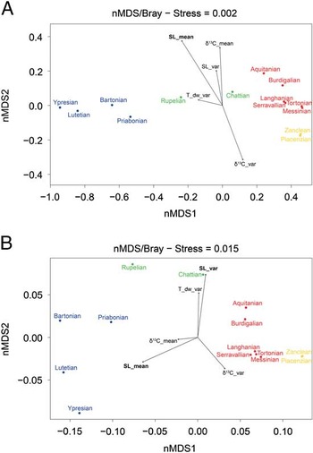
Figure 10 Similarity among time periods for community composition in relation to environmental variables. nMDS ordination of time periods as a function of the presence/absence of coral genera (A) and as a function of relative abundance of functional trait states (B). Time intervals: blue, Eocene; green, Oligocene; red, Miocene; yellow, Pliocene. Rotational vectors for environmental variables are fitted to the ordination axis to reveal their corresponding relationship to time intervals; significant environmental factors are highlighted in bold (p=0.05).
Discussion
Biodiversity hotspots are regions with sharply higher diversity relative to surrounding regions. They vary temporally and spatially due to the interplay of modern and historical ecological, geological, and environmental factors. Biodiversity itself is not only a measure of taxonomic richness but also of organismal and ecosystem functionality. Here we couple the taxonomic and functional development of coral communities with environmental dynamics of biodiversity hotspots to understand what drives biogeographic patterns of biodiversity and species–area relationships over time. Our findings show the Central Indo-Pacific biodiversity hotspot originated during the Oligocene. This provides a new working hypothesis for the timing of origination of the present-day Indo-Pacific diversity hotspot, clarifies previous estimates of the timing of origination (Wilson and Rosen Reference Wilson and Rosen1998; Renema et al. Reference Renema, Bellwood, Braga, Bromfield, Hall, Johnson, Lunt, Meyer, McMonagle, Morley, O’Dea, Todd, Wesselingh, Wilson and Pandolfi2008; McMonagle Reference McMonagle2012; Santodomingo et al. Reference Santodomingo, Renema and Johnson2016) and gives insight into underlying mechanisms of hotspot development. Specifically, our data show variable rates in the accumulation of diversity through time and decoupling of taxonomic and functional diversity patterns.
Taxonomic Diversity
Low diversity in the Eocene followed by a rapid increase in the Oligocene and earliest Miocene (Rupelain to Aquitanian, Figs. 5A and 7) and the maintenance of relatively high diversity throughout the rest of the Miocene and Pliocene results from the interactions between origination and extinction rates (Fig. 7). It should be noted that the increase in diversity might be underestimated due to sampling of indurated limestone lithologies, which represent potentially the most diverse depositional environments in the Central Indo-Pacific (Wilson Reference Wilson2015). Limestones are challenging for studying macrofossils due to diagenetic alteration (Wright and Burgess Reference Wright and Burgess2005), and this process is suggested by the undersampling of the Aquitanian corals in our new fossil collection (Fig. 4). As such, more complete sampling of limestone lithologies would enhance the observed increase in taxonomic diversity.
The complex interplay among, and co-occurrence of, global and local tectonic, eustatic, oceanographic, and climatic events (TECO events of Rosen Reference Rosen1984) makes it challenging to determine the precise drivers of the observed patterns in origination and extinction as well as coral community composition (Wilson Reference Wilson2008). Nonetheless, increasing taxonomic diversity from the Eocene to Pliocene (Fig. 5A) appears to be negatively (Fig. 5C) associated with mean global sea level (Fig. 10A). An overall decrease in global sea level from the Eocene to the Oligocene (Fig. 5C) coincides with local tectonics, such as continental collision and regional uplift (Hall Reference Hall2002; Hutchison Reference Hutchison2004), that resulted in an increase in shallow-marine habitats. It is possible that a relatively high sea level largely constrained coral proliferation and diversification in the Eocene (Fig. 5C). We propose that falling sea level from the Eocene until the late Oligocene largely promoted coral proliferation and diversification by increasing the area of shallow-water habitats ideal for coral growth (Fig. 11) (Hall Reference Hall2001; Renema et al. Reference Renema, Bellwood, Braga, Bromfield, Hall, Johnson, Lunt, Meyer, McMonagle, Morley, O’Dea, Todd, Wesselingh, Wilson and Pandolfi2008; Wilson Reference Wilson2008). Extinction at the end of the Eocene likely reflects an alternative response of some taxa to the environmental changes associated with abrupt sea-level fall; however, the loss of these taxa is not enough to negate the general increasing trend in taxonomic diversity over time (Fig. 5A).

Figure 11 Plot of the area of coral-dominated carbonates (log) and sea level from the early Eocene to the Pliocene of the Central Indo-Pacific.
During the late Oligocene–early Miocene, the greatest increase in taxonomic diversity occurs (Fig. 5A), likely representing the accumulation of taxonomic diversity due to sustained, relatively higher origination rates from the Bartonian to the Aquitanian (Fig. 7). This increase in taxonomic diversity coincides with the abrupt regional increase in the relative area of coral-dominated carbonates (Wilson Reference Wilson2008), resulting from the transition of local reef habitats from large carbonate platforms dominated by foraminifera in the Eocene to more isolated and shallower platforms dominated by corals in the Miocene (e.g., Wilson Reference Wilson2002; Mihaljević et al. Reference Mihaljević, Renema, Welsh and Pandolfi2014). Observation of coral diversity peaking in the Aquitanian, when the relative area of coral-dominated carbonates abruptly increased (Wilson Reference Wilson2008), is consistent with a species–area relationship, in which the number of species is expected to increase as the amount of available habitat space increases (Rosenzweig Reference Rosenzweig1995). Lack of reef framework in the Central Indo-Pacific until the Aquitanian (Wilson Reference Wilson2002, Reference Wilson2008; Mihaljević et al. Reference Mihaljević, Renema, Welsh and Pandolfi2014) suggests that the Central Indo-Pacific diversity hotspot originated (i.e., increased faunal turnover and magnitude of diversity) in habitats characterized by low abundance but moderate diversity of corals (Mihaljević et al. Reference Mihaljević, Renema, Welsh and Pandolfi2014). The positive logarithmic trend between the MSD and area of carbonate structures (Fig. 6) supports this hypothesis.
Interestingly, there is a lack of a species–area relationship from the early Miocene onward. Coral diversity continued to increase through the Pliocene, despite a decrease in origination rates from the early Miocene and decreasing area of coral-dominated carbonates from the middle Miocene (Fig. 6). If the area of coral-dominated carbonates is considered a proxy for suitable habitat, it is plausible that as habitat availability declined from the early Miocene, physical barriers could have developed, creating isolation and promoting speciation (i.e., continued diversification) (Keith et al. Reference Keith, Baird, Hughes, Madin and Connolly2013). An increase in habitat complexity could sustain a continued, albeit relatively lower, rate of diversification into the Pliocene (Guégan et al. Reference Guégan, Lek and Oberdorff1998; Báldi Reference Báldi2008). Additionally, if habitat area was reduced and coral taxa were confined to coexist in a smaller area, increased pressure from biological interactions (e.g., competition) also could have contributed to low diversification rates (e.g., Rosenzweig Reference Rosenzweig1995) and the lack of a species–area relationship through to the Pliocene.
The decrease in shallow-marine habitats from the middle Miocene is likely related to the complex interactions between continued falling sea level and regional tectonic uplift. From the Eocene to the Oligocene, the interaction of falling global sea level and regional uplift resulted in the expansion of shallow-marine habitats by collectively reducing regional sea level. By the middle Miocene, however, the effects of this interaction appear to have changed, as the trajectory between global sea level and the area of coral-dominated carbonates reverses (Fig. 11). We propose that, through the interplay of falling global sea level and regional tectonic uplift, regional sea level reached a critical (low) threshold in the Central Indo-Pacific around the middle Miocene, after which continued sea-level fall (and uplift) began to decrease the area of shallow-marine habitats suitable for corals. This transition exemplifies the complexity of sea-level and tectonic interactions and their cumulative effect on ecology over time.
In addition to the interaction of global sea level and local tectonics, other global and local environmental variables, with less continuous records than sea level, could have influenced coral diversity trends over time. For instance, changes in ocean chemistry might have promoted the abrupt increase in coral diversity from the Rupelian to the Aquitanian (across the Oligocene/Miocene boundary). During this time, the global seawater Mg/Ca ratio (a proxy for carbonate precipitation for which higher values favor the precipitation of aragonite over calcite) was increasing, and local salinity became more consistent due to more constant terrestrial runoff driven by a climatic shift—from seasonal to ever-wet conditions—over the Oligocene/Miocene boundary (Stanley and Hardie Reference Stanley and Hardie1998; Morley Reference Morley2000, Reference Morley2011; Morley et al. Reference Morley, Morley and Restrepo-Pace2003). The shift to more consistent, less seasonably variable conditions would lead to more favorable, less stressful shallow-water environmental conditions, potentially promoting coral proliferation and diversification (Wilson Reference Wilson2008).
Johnson et al. (Reference Johnson, Renema, Rosen and Santodomingo2015) highlighted that imprecise dating methods in early Central Indo-Pacific collections led to some genera being placed in incorrect time periods. Considering these results, the high extinction and origination rates observed in our data at the end of the Miocene and beginning of the Pliocene, respectively, should both be lower. Consequently, lower extinction rates would correspond to relatively higher diversity and limited turnover throughout the Miocene and Pliocene, corroborating findings of previous studies (Johnson et al. Reference Johnson, Renema, Rosen and Santodomingo2015; Santodomingo et al. Reference Santodomingo, Renema and Johnson2016). Although these findings would slightly alter magnitude of the observed diversity patterns in the latest Miocene and early Pliocene, they do not affect the estimated timing of origination of the Central Indo-Pacific biodiversity hotspot, which our results show to be in the late Oligocene.
Functional Diversity
Intriguingly, observed patterns in taxonomic diversity are decoupled from patterns in functional diversity. Despite significant fluctuations in taxonomic diversity, functional diversity remained relatively stable (Fig. 5B), irrespective of temporal variations in trait abundances and turnover rates (Fig. 9 and Supplementary Fig. 2). Taxonomic and functional diversity trends could be expected to be similar if new traits are arising as the result of the development of new taxa (or vice versa) (Naeem and Wright Reference Naeem and Wright2003; Petchey and Gaston Reference Petchey and Gaston2006; Villéger et al. Reference Villéger, Miranda, Hernández and Mouillot2010). Our finding of high stability in functional diversity during periods of high diversification contradicts these expectations and points toward high functional redundancy, suggesting that species added to the community occupy the same functional space (i.e., have similar traits) as already existing species (Mayfield et al. Reference Mayfield, Bonser, Morgan, Aubin, McNamara and Vesk2010; Cadotte et al. Reference Cadotte, Carscadden and Mirotchnick2011).
The co-occurrence of species occupying the same functional space can be facilitated through expansion of habitat area, resulting in relaxation of species competition (e.g., space). As previously discussed, global sea-level changes combined with local tectonics contributed to the expansion of shallow-marine habitats suitable for coral growth. The influence of the sea level on abundance of functional trait states is clearly illustrated by the separation of Eocene–Oligocene and Miocene–Pliocene functional communities by significant sea-level mean and variance vectors (Fig. 10B). Additionally, the reported increase in habitat complexity (Mihaljević et al. Reference Mihaljević, Renema, Welsh and Pandolfi2014) might further promote functional redundancy in corals. While most functional trait states were present in all time intervals, that is, functional diversity through time is constant, their relative abundances varied through time in response to environmental changes. Considering high morphological plasticity of corals, simple turnover of already existing trait states would allow for rapid adaptation to the emerging habitat availability and complexity without the “need” for new adaptations. Thus, functional redundancy might have contributed to the ~28 Myr-long persistence of the Central Indo-Pacific biodiversity hotspot through promoting ecosystem stability following declines in taxonomic diversity (Fonseca and Ganade Reference Fonseca and Ganade2001; Guillemot et al. Reference Guillemot, Kulbicki, Chabanet and Vigliola2011).
Despite the decoupling of taxonomic and functional trait diversity patterns, both taxonomic and functional trait composition become more dissimilar as the time separating assemblages increases (Fig. 8A,C). This ubiquitous increase in dissimilarity of assemblages with increasing time is likely not solely driven by random accumulation of diversity over time, but might also reflect the development of reef communities in response to habitat availability, for example, diversity increases with increasing habitat availability (Tager et al. Reference Tager, Webster, Potts, Renema, Braga and Pandolfi2010). Temporal trends in taxonomic, trait, and environmental conditions are not linear per se (i.e., taxonomic diversity has not increased at a steady rate over time, nor has sea level linearly lowered), and fluctuations in these factors likely have interactive effects on coral assemblages over time (Bromfield and Pandolfi Reference Bromfield and Pandolfi2011), resulting in dissimilar communities from the Eocene to the Pliocene (Fig. 8B,D).
Although cluster analyses show increasing dissimilarity with time for both taxonomic and functional trait assemblages, the results also reveal that the pattern of dissimilarity is not the same for both taxonomic and functional assemblages (Fig. 8B,D). Most notably, Chattian generic composition was more similar to that of younger time periods (Miocene and Pliocene) than to the Eocene, whereas the Chattian functional composition was more similar to the older (Eocene) period (Fig. 8B,D). This implies that the biggest taxonomic turnover (Rupelian–Chattian) is largely disconnected from functional trait dynamics. The decoupling of Chattian taxonomic and functional assemblages suggests that the response of corals to expanding habitats in the Chattian was characterized by the local appearance of new taxa (leading to the grouping of this era with the younger time periods) that maintained the same functional space as those in the pre-Chattian (therefore maintaining functional similarity to older time periods). In contrast, further expansion and diversification of suitable habitats in the Aquitanian led to the emergence of new taxa that was accompanied by changes in the functional space of the Aquitanian coral communities (Renema et al. Reference Renema, Bellwood, Braga, Bromfield, Hall, Johnson, Lunt, Meyer, McMonagle, Morley, O’Dea, Todd, Wesselingh, Wilson and Pandolfi2008; Wilson Reference Wilson2008; Mihaljević et al. Reference Mihaljević, Renema, Welsh and Pandolfi2014). The decoupling of taxonomic and functional diversity means that (1) functional trait dynamics are not dependent on taxonomic dynamics (Figs. 5 and 8), and (2) taxonomic and trait dynamics can be influenced differently by the same environmental factors (Fig. 10).
Mechanisms of Increase in Coral Reef Area during the Origin of the Hotspot
The abrupt increase in reef area in the late Oligocene and especially the early Miocene is associated with the proliferation of already present taxa and origination/immigration of new taxa. The strong positive correlation between coral-dominated area and MSD indicates that the origination/immigration of new taxa was undoubtedly a key mechanism. However, the proliferation of already present taxa must also have contributed to the abrupt increase in coral-dominated carbonates because: (1) increases in the area of coral-dominated carbonates and coral diversity are not proportional through time, and (2) Chattian communities are functionally more similar to communities older than the Miocene. For example, a comparison of the contribution of already present and new taxa to the relative abundance of colony growth trait states (branching, massive, platy, discoid, and cup-shaped)—a proxy for coral area—revealed that taxa already present in the Chattian contributed more to the relative abundance of all coral growth forms than did new taxa. The same is true in the Aquitanian, with the exception that new taxa with platy and discoid growth forms, which tend to be common in turbid (oligophotic) environments (Rosen et al. Reference Rosen, Aillud, Bosellini, Clack, Insalaco, Valldeperas and Wilson2002; Browne et al. Reference Browne, Smithers and Perry2012; Novak et al. Reference Novak, Santodomingo, Rösler, Di Martino, Braga, Taylor, Johnson and Renema2013), contribute more than already present taxa with these growth forms (Table 3). These patterns suggest that the Central Indo-Pacific biodiversity hotspot has developed in oligophotic conditions in two phases: (1) in the Chattian through proliferation of coral genera already present since the Rupelian, and (2) in the Aquitanian through the expansion of existing taxa as well as through the origination/immigration of new genera.
Table 3 Percentage contribution of old and new taxa to relative abundances of coral growth forms. Old taxa refers to 46 genera already present in Rupelian.
Conclusions
Our study shows that the Central Indo-Pacific has persisted as a biodiversity hotspot since the Chattian (~28 Myr), which is ~5 Myr earlier than previously thought. We postulate that functional redundancy, seen through the decoupling of taxonomic and functional diversity, potentially contributed to the persistence of the hotspot by promoting ecosystem stability. An increase in shallow-marine habitats suitable for coral growth, resulting from the interplay of global sea level and regional tectonics, seems to have driven this diversification of Central Indo-Pacific corals, which, through proliferation of already present genera, immigration, and origination of new ones contributed to the expansion of reef area. Therefore, the history of the Central Indo-Pacific highlights that marine biodiversity hotspots develop through a complex interplay of proliferation, accumulation, and origination of coral genera.
Acknowledgments
We acknowledge financial contributions from Petroliam Nasional Berhad (Petronas), Pearl Energy, the University of Queensland (UQ) International Scholarship (UQI) 2011–2014, the UQ Collaboration and Industry Engagement Fund, UQ Centre for Marine Science, the Australian Research Council Centre of Excellence for Coral Reef Studies, and the Winifred Violet Scott Trust. We also thank the State Planning Unit in Kuching, Malaysia for allowing us to conduct research in Sarawak, and the National Parks and Nature Reserves for a research permit for the Gunung Mulu National Park. Special thanks for logistical, physical, and all other help during seven field trips in Sarawak, Malaysia, and the islands of Cebu and Negros, Philippines, go to: Peter Lunt, the Gunung Mulu National Park staff (especially Brian Clark), Luke Southwell, Hollystone Quarry Sdn. Bhd. staff, people from the Long Jeh community, Brian Beck, King King Ting, the Mines and Geosciences Bureau in Manila and Mandaue City (especially Yolanda Aguilar and Abraham R. Lucero), Felix G. Nepomucedo, and Jack Coates-Marnane. We would also like to thank Simon Blomberg, Etienne Laliberte, Sandrine Pavoine, and Juan Carlos Ortiz for discussions about the statistical analysis. We thank Bas de Boer and James Zachos for access to raw environmental data. Special thanks to Aaron Hunter, Brigitte Sommer, Eugenia M. Sampayo, three anonymous reviewers and the editor for their comments on earlier versions of this article.
Supplementary Material
Data available from the Dryad Digital Repository: http://dx.doi.org/10.5061/dryad.3k5v6