


Introduction
The molluscan class Gastropoda (snails and slugs) is one of the largest, most diverse groups of animals on Earth, with an estimated 32,000 to 40,000 named living gastropod species (Appeltans et al. Reference Appeltans, Ahyong, Anderson, Angel, Artois, Bailly, Bamber, Barber, Bartsch, Berta, Błażewicz-Paszkowycz, Bock, Boxshall, Boyko, Brandão, Bray, Bruce, Cairns, Chan, Cheng, Collins, Cribb, Curini-Galletti, Dahdouh-Guebas, Davie, Dawson, De Clerck, Decock, De Grave, de Voogd, Domning, Emig, Erséus, Eschmeyer, Fauchald, Fautin, Feist, Fransen, Furuya, Garcia-Alvarez, Gerken, Gibson, Gittenberger, Gofas, Gómez-Daglio, Gordon, Guiry, Hernandez, Hoeksema, Hopcroft, Jaume, Kirk, Koedam, Koenemann, Kolb, Kristensen, Kroh, Lambert, Lazarus, Lemaitre, Longshaw, Lowry, Macpherson, Madin, Mah, Mapstone, McLaughlin, Mees, Meland, Messing, Mills, Molodtsova, Mooi, Neuhaus, Ng, Nielsen, Norenburg, Opresko, Osawa, Paulay, Perrin, Pilger, Poore, Pugh, Read, Reimer, Rius, Rocha, Saiz-Salinas, Scarabino, Schierwater, Schmidt-Rhaesa, Schnabel, Schotte, Schuchert, Schwabe, Segers, Self-Sullivan, Shenkar, Siegel, Sterrer, Stöhr, Swalla, Tasker, Thuesen, Timm, Todaro, Turon, Tyler, Uetz, van der Land, Vanhoorne, van Ofwegen, van Soest, Vanaverbeke, Walker-Smith, Walter, Warren, Williams, Wilson and Costello2012; Rosenberg Reference Rosenberg2014). With a fossil record that extends to the Cambrian, gastropods are the subject of major taxonomic and evolutionary research worldwide. Their long fossil record makes them an attractive model system for the study of macroevolutionary tempo and mode (Bieler Reference Bieler1992), and their accretionary, coiling form means that the shell preserves an essentially complete record of ontogeny up until the time of death. However, existing morphometric methods fail to capture key descriptive parameters of this spiral, and the full potential of the group for macroevolutionary studies of morphology has been only partially realized.
Mathematical analysis of shape (morphometrics) is a powerful tool in biology and paleobiology that provides data for taxonomy and biostratigraphy, phylogenetic analyses, evolutionary studies, and paleoenvironmental reconstruction. Morphometrics has been employed successfully to study the evolution of other molluscan groups such as bivalves (Claxton et al. Reference Claxton, Wilson, Mackie and Boulding1998; Crampton and Maxwell Reference Crampton, Maxwell, Harper, Taylor and Crame2000; Marquez et al. Reference Márquez, Robledo, Peñaloza and Van der Molen2010; Collins et al. Reference Collins, Crampton and Hannah2013; Aguirre et al. Reference Aguirre, Richiano, Álvarez and Farinati2016) and the planispiral cephalopods (Gerber et al. Reference Gerber, Neige and Eble2007, Reference Gerber2011). Helicospiral gastropods (as a group) have greater variability in their geometry (see Fig. 1 for a range of forms; see also Raup Reference Raup1966: fig 4) than either bivalves or planispiral cephalopods, but with modern computing methods, variation alone should not constitute an intractable problem for morphometric analysis.
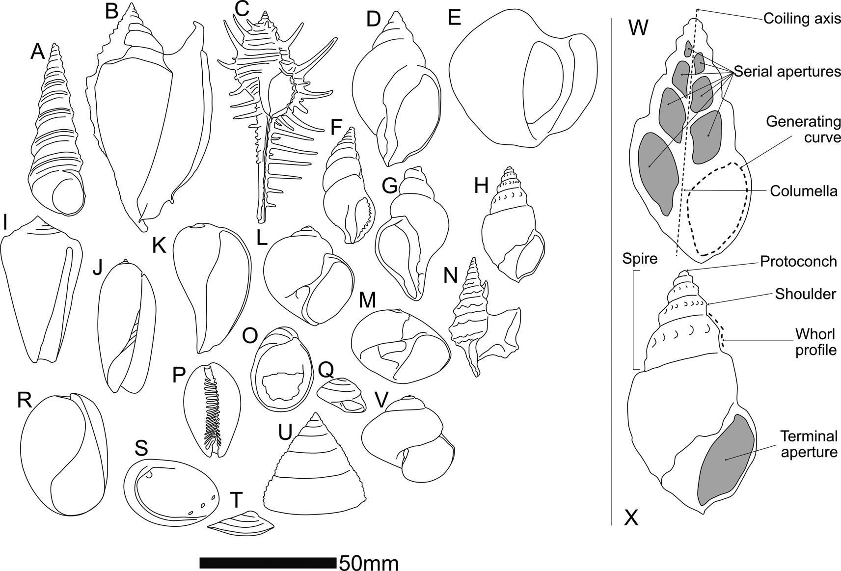
Figure 1. A cross section of gastropod morphological diversity. A, Turritella sp. B, Euprotomus aratrum (Röding, Reference Röding1798). C, Murex altispira Ponder & Vokes, Reference Ponder and Vokes1988. D, Neptunea antiqua (Linnaeus, Reference Linnaeus1758). E, Conchothyra parasitica Hutton, Reference Hutton1877. F, Colubraria tortuosa (Reeve, Reference Reeve1844). G, Neptunea angulata (Wood, Reference Wood1848). H, Tylospira scutulata (Gmelin, Reference Gmelin and Gmelin1791). I, Conus consors G. B. Sowerby I, Reference Sowerby and Sowerby1833. J, Oliva miniacea (Röding, Reference Röding1798). K, Ficus subintermedia (d'Orbigny, Reference d'Orbigny1852). L, Eunaticina umbilicata Quoy & Gaimard, Reference Quoy and Gaimard1832. M, Neverita didyma (Röding, Reference Röding1798). N, Aporrhais pespelecani (Linnaeus, Reference Linnaeus1758). O, Nerita albicilla Linnaeus, Reference Linnaeus1758. P, Lyncina lynx (Linnaeus, Reference Linnaeus1758). Q, Steromphala umbilicalis (Da Costa, Reference Da Costa1778). R, Bulla ampulla Linnaeus, Reference Linnaeus1758. S, Haliotis tuberculate Linnaeus, Reference Linnaeus1758. T, Patella pellucida Linnaeus, Reference Linnaeus1758. U, Trochus maculatus Linnaeus, Reference Linnaeus1758. V, Janthina janthina (Linnaeus, Reference Linnaeus1758). W, X (not to scale) two views of Tylospira scutulata (W in cross section, X an exterior view), bearing labels for anatomical features discussed in this paper.
That said, differences in shell form between higher-level gastropod taxa are in many cases too great to allow comparison via current geometric morphometric methods. At the same time, groups like the Stromboidea (e.g., Fig. 1B [Strombidae], E and H [Struthiolariidae], N [Aporrhaidae]), many of which feature spectacular spikes, spikes, knobs, wings, and calluses as part of their adult (but not juvenile) shell, are difficult to compare with each other using geometric morphometrics, even within the same genus, although we know from molecular methods that they are closely related. Three issues that have confounded geometric morphometric analysis of gastropods to date are:
1. consistent identification of biologically homologous landmarks within individuals through ontogeny and across taxa;
2. allometry of the generating curve; and
3. different numbers of whorls between individuals.
Landmark and semilandmark methods require at least two (for 2D) or three (for 3D) biologically homologous, consistently locatable point(s) on the shell surface by which to orient themselves. The sculptural elements that would seem to provide these landmarks typically fail to be strictly homologous (Merle Reference Merle2005; Liew et al. Reference Liew, Kok, Schilthuizen and Urdy2014) in a way that functions well with the geometric morphometric paradigm, even though the shell is overall a part of the animal that is homologous between individuals. External shell shape can be just as easily dictated by environmental factors as by genetics (e.g., Dalziel and Boulding Reference Dalziel and Boulding2005; Brookes and Rochette Reference Brookes and Rochette2007; Harasewych and Petit Reference Harasewych and Petit2013), and the protoconch, which would theoretically seem to be an excellent starting place for truly homologous landmarks, is often broken or lost, or smooth and featureless.
Methods such as placing landmarks at sutures between whorls in two-dimensional (2D) images of snails (e.g., Van Bocxlaer and Schultheiß Reference Van Bocxlaer and Schultheiß2010; Vaux et al. Reference Vaux, Crampton, Marshall, Trewick and Morgan-Richards2017, Reference Vaux, Trewick, Crampton, Marshall, Beu, Hills and Morgan-Richards2018) or employing Fourier analysis of a 2D outline of a snail (e.g., Roy et al. Reference Roy, Balch and Hellberg2001; McClain Reference McClain2004; Wilson et al. Reference Wilson, Glaubrecht and Meyer2004) give an approximation of the snail's shape but ignore its spiraling nature and assume that the profile of the shell as viewed in the traditional spire-up, aperture-facing view for illustration is a single, biologically meaningful contour. This approach has applications in taxonomic and, to some extent, ecological analysis, but does not provide sufficient coverage of form for more detailed morphological studies and fails to acknowledge the role of ontogeny in producing the final form of the shell. Landmarks on a profile comprising successive whorls are also highly correlated—they are formed by the same generating curve, albeit one that might change shape through ontogeny. Combining all landmarks into one profile causes arithmetic redundancy in subsequent shape analyses. Landmark analyses of this kind are also confounded by the whorl-number problem, as landmark studies require the same number of landmarks for every specimen. These issues have been discussed and summarized by authors such as Stone (Reference Stone1998) and Johnston et al. (Reference Johnston, Tabachnick and Bookstein1991).
The aperture, or serial “apertures” up the spire as created by sectioning a shell down its columella (or umbilicus), does approximate a biologically meaningful contour, the generating curve, and this is amenable to 2D morphometric analysis. This curve records the position of the mantle edge that forms new growth increments of shell (see Schindel [Reference Schindel, Ross and Allmon1990] for a discussion of the relationship between the true terminal aperture and sectioned apertures). However, comparing a single aperture (sectioned or terminal) from any given snail with that of other snails is not sufficient to describe the form of the snail, and the generating curve (the margin of the soft parts along which the shell is produced) changes shape and orientation through ontogeny. Attempting to make up for this in a geometric morphometric framework by comparing the shapes of multiple apertures up the spire runs into the number-of-whorls mismatch issue, further complicated by frequent damage to the shell at both ends. In any real specimen, the likelihood of the entire set of whorls being preserved is low—especially for fossil specimens.
In this study, we take an approach that combines the coiling parameter paradigm from theoretical shell morphology with a variation on geometric morphometrics to produce an empirical morphospace. The centroid (“centre of gravity” in Thompson [Reference Thompson1942]); Schindel [Reference Schindel, Ross and Allmon1990]) of the generating curve is used as a semilandmark to trace the ontogeny of the shell, rather than an external sculptural element or internal point along the generating curve. This was termed the “aperture trajectory” by Stone (Reference Stone1998). In our present study, centroids are measured for serial apertures down the shell and used to calculate coiling parameters in a cylindrical coordinate space, analogous to those of Raup (Reference Raup1966). Use of the centroid circumvents the necessity of identifying a consistent landmark on a shell and does not require each whorl, or aperture, or the generating curve underlying both, to be the same shape through ontogeny (a property known as self-similarity or gnomonic growth in earlier literature or isometric growth in more modern parlance). The use of coiling parameters, rather than x,y landmarks or semilandmarks in a Cartesian space, avoids the whorl-number problem, because each snail, regardless of number of whorls, can be described by the same number of mathematically independent variables, summarizing how the generating curve migrates through space during ontogeny.
Theoretical and Empirical Shell Models and Morphospaces
Theoretical shell models (e.g., Raup and Michelson Reference Raup and Michelson1965; Raup Reference Raup1966; Okamoto Reference Okamoto1984; Løvtrup and Løvtrup Reference Løvtrup and Løvtrup1988; Hutchinson Reference Hutchinson1989, Reference Hutchinson1990; Savazzi Reference Savazzi1990; Stone Reference Stone1995; Tursch Reference Tursch1997; Rice Reference Rice1998; McGhee Reference McGhee1999; Hammer and Bucher Reference Hammer and Bucher2005; Urdy et al. Reference Urdy, Goudemand, Bucher and Chirat2010; Noshita et al. Reference Noshita, Asami and Ubukata2012; Noshita Reference Noshita2014) are morphological models (as opposed to evolutionary models) that seek to parameterize shell form in order to model shell growth. The product of a theoretical shell model is a theoretical shell morphospace—the model (which may or may not be based on a set of measurements) defines the axes of the morphospace, and then measurements from specimens can be plotted within it. This kind of morphospace could provide an ideal starting point for developing a morphometric system to describe real shells—after all, one should be able to plot real shells in a morphospace once it has been constructed (successful examples include: McGhee Reference McGhee1980; Gerber et al. Reference Gerber, Neige and Eble2007, Reference Gerber2011). So why has this not been applied to gastropods? Schindel (Reference Schindel, Ross and Allmon1990) proposes that it is because real gastropod shells cannot be placed in any of the theoretical gastropod shell morphospaces that have been proposed—the parameters of the models are not sufficient to summarize real gastropod shells or cannot practically be measured from real gastropod shells. However, we propose that perhaps the model that has been used is not the best fit to real snail shapes.
Theoretical shell models vary widely, but most assume a logarithmic helicospiral as a basis. Thompson (Reference Thompson1942: p. 771), who took the logarithmic model from Moseley (Reference Moseley1838), explains that the logarithmic helicospiral, such as that seen in Turbo Linnaeus, Reference Linnaeus1758, can be thought of as (paraphrased): a spiral in which the radius vector is inclined to the coiling axis at a constant angle β, forming a logarithmic spiral wrapped upon a cone, and which is similar in shape the whole way along.
The molluscan shell form as thus described is conceptualized as a translation of a closed generating curve about an axis, such that the generating curve does not change in shape but increases in size. This isometric (“gnomonic,” in Thompson's [Reference Thompson1942] terminology) growth is an underlying assumption of almost all shell-growth models, largely following Raup (Reference Raup1966), in which this mode of growth was accepted (Stone Reference Stone1996).
Two assumptions, therefore, underlie our current understanding of (most) molluscan shell growth:
• that shells grow exponentially, tracing a logarithmic helicospiral; and,
• that the generating curve of a shell is a fixed shape
The first assumption is dependent on the second—the identification of a logarithmic helicospiral is founded on the properties of the curve traced by some given point that is typically on the exterior of the shell—a shoulder nodule, a spiral cord, a lineation, or the suture between whorls. Whereas it is theoretically possible to change the shape of the aperture while maintaining the logarithmic spiral, the shape of every whorl affects the shape of the whorl that comes after, and thus allometric growth can and often does affect the position of the centroid of each successive whorl (Fig. 2). (We do not consider those cases where the animal resorbs and remodels the inside of older whorls during ontogeny—here the remodeled apertures were not digitized). Because of non-isometric growth, in many gastropods, distinctive features of the final whorls of an adult shell are not necessarily present on successively (ontogenetically) younger whorls. This is not a new finding (e.g., McGhee Reference McGhee1980; Schindel Reference Schindel, Ross and Allmon1990), but authors have continued to use the logarithmic helicospiral as a basis for their models, despite having identified deviation from it as a potential source of error.
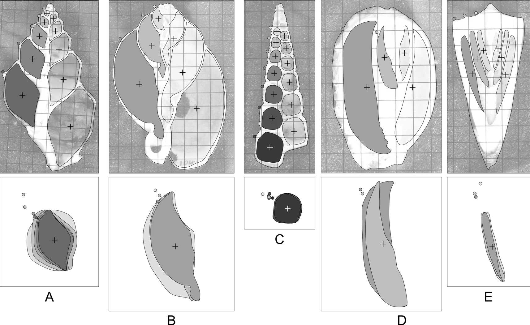
Figure 2. Shape variation in apertures of sectioned gastropods: A, Struthiolaria papulosa; B, Semicassis pyrum (Lamarck, Reference Lamarck1822); C, Maoricolpus roseus (Quoy & Gaimard, Reference Quoy and Gaimard1834); D, Cypraea sp.; E, Conus sp. Grids on images are 5 mm squares. Crosses denote aperture centroids. Filled circles on the shell outline denote the shoulder of the whorl. Below each shell, the inset box takes the filled apertures from the left side of each shell (for clarity of illustration only: apertures from both sides of the shell are used in analyses), centers, and scales them to unit area. The degree of allometry varies between species, as does the relative position of the external “landmark” that would be used to calculate whorl parameters. Some shells (e.g., C,E) are very close to isometric, others (e.g., A,D) display marked allometry. Without cross-sectional views of the shell, it is difficult to assess the degree of allometry for any given species.
An additional issue concerns the use of landmarks on the exterior surface of the shell to define the helicospiral: the external surface is never coincident with the “true” generating curve and may be modified by thickened shell, spines, ribs, flanges, callus, and so on. The contour on the inside of the shell cavity is the best available approximation of the generating curve (if one considers the extrapallial space to be the “organ” that produces the shell, then the interior surface of the shell, where the soft parts anchor, will provide a more conservative representation of the shape of that organ across taxa than the exterior curve, which incorporates sculptural elements in some but not all individuals or taxa), although as observed by previous authors, the section of that curve revealed by a sagittal cross section of the whole shell typically is at an angle to the true generating curve (McNair et al. Reference McNair, Kier, LaCroix and Linsley1981; Schindel Reference Schindel, Ross and Allmon1990; Vermeij Reference Vermeij2010). Landmarks on the internal contour, however, are difficult to establish, as the internal contour is typically smoothly rounded, with few points that could be used as homologous landmarks and few constraints that could be used to anchor simple geometrical semilandmarks (“Type Two” landmarks of Bookstein [Reference Bookstein1991]).
The present study can be considered an empirical shell morphospace of coiling, in that it starts with empirical measurements and looks for a best-fit model of growth, rather than starting with a theoretical model of growth and taking measurements to feed into it.
Methods
The parameters we define and use are analogous, conceptually rather than mathematically, to the parameters set out by Raup (Reference Raup1966) and used subsequently in other studies in different formulations (e.g., McGhee Reference McGhee1980; McClain Reference McClain2004; Gerber et al. Reference Gerber, Neige and Eble2007). We calculate the rate of translation (Te) using aperture centroids, and rate of whorl expansion (We), rate of increasing distance of the aperture from the coiling axis (De), and generating curve shape (Se) using the digitized aperture outline. The subscript e on our parameters differentiates them from the original Raupian formulation by emphasizing that they are derived from empirical measurements, not from Raup's original equations, despite describing analogous aspects of spiral form.
One hundred seventy-six sagittal sections of fossil and modern shells make up the study dataset. Imaging was either by physical sectioning and photography, or in the case of rare fossil material, by synchrotron radiation computed microtomography. We examined a range of shell forms, including fusiform, turriculate, and trochiform. Supplementary Table S1 lists the specimens included, method of imaging, and relevant parameters.
The central axis of the cylindrical coordinate system is the snail's coiling axis. r is then the distance of the aperture centroid from the coiling axis, and y the vertical distance along the coiling axis from the first measurement. θ, the angle between a given aperture and the aperture before, is measured from an arbitrary zero, which is necessary, as the apex or protoconch of the shell is almost always lost or, even where present, may be too small to measure.
We use the following notation (illustrated in Fig. 3):
• θ is the angle around the coiling axis from the last aperture, measured in radians
• rθ is the distance from the coiling axis at θ
• yθ is the distance along the coiling axis at θ
• r0 is r at θ = 0 (i.e., the distance from the coiling axis of the first measured aperture)
• y0 is y at θ = 0 (set usually to 0)
Given this,
• We is the rate of whorl expansion (i.e., rate of aperture area increase);
• Te is the rate of downward growth of the spiral;
• De is the rate of movement of the aperture away from the coiling axis; and
• Se is the rate of change of the shape of the aperture (described using principal components analysis on morphometric data—in our case, from a fast Fourier transform [FFT] of the aperture coordinates).
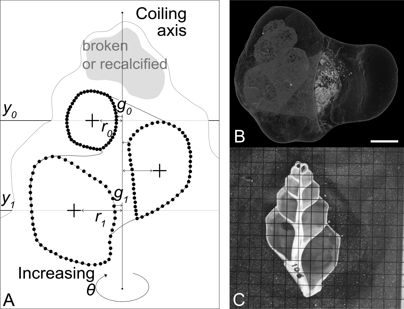
Figure 3. Parameters captured by semilandmarking serial apertures, and the two different methods of imaging. A, Diagrammatic representation of a sectioned shell. Small black circles indicate manually placed points (semilandmarks). From the semilandmarks, the centroid of each aperture (cross) can be calculated. The first centroid is placed at y 0; r 0 and g 0 are then measured as the distance from the coiling axis to the centroid and the coiling axis to the closest edge of the aperture at y 0 respectively. One full revolution later, y 1, r 1, and g 1 can be measured. B, Synchrotron CT scan of Conchothyra parasitica (scale bar, 10 mm). This can be digitally sectioned to produce an image similar to the photograph in C. C, Physically sectioned specimen of Struthiolaria papulosa (grid: 5 mm squares).
Landmark data capture is undertaken in tpsDig (Rohlf Reference Rohlf2017), a data capture program that has become a de facto standard in morphometric studies. Two points are placed along the coiling axis (determined visually). Serial “apertures” up the spire are digitized using an arbitrarily chosen 50 (manually placed, and then adjusted using tpsDig to be equally spaced) points per curve. As many apertures as possible are captured for each specimen, avoiding apertures that are obviously damaged or have been internally recalcified or otherwise remodeled.
The resulting .tps file is read into R (R Core Team 2020) for analysis. The workflow can be described as follows:
1. Read in images and .tps file, and process metadata, landmarks, and semilandmark curves.
2. Calculate and record the centroid of each digitized aperture for each specimen.
3. Calculate and record the area of each digitized aperture for each specimen.
4. Rotate each specimen so that the coiling axis is aligned vertically (to the y-axis of the coordinate system).
5. Measure and record the width between the inner edge of each aperture and the coiling axis.
6. Translate all points from Cartesian space to cylindrical space. Every specimen's first (ontogenetically youngest) digitized aperture centroid is pinned to 0. The polar axis is defined by the two landmarks delineating the coiling axis of the specimen.
7. Each of the parameters Te (translation), We (whorl expansion), and De (distance of aperture from coiling axis) is a rate of change that can be calculated using a number of different models: calculate each parameter five times using linear, logarithmic, power law, exponential, and quadratic models, and then compare the fit of the five different models to the data. The five models are (in code and equation form):
a. Linear: lm(y ~ theta)
(1) $$y = {\rm \alpha \theta } + {\cal N}\lpar {0\comma \;{\rm \;\sigma }} \rpar $$
b. Quadratic: lm(y ~ poly(theta, 2))
(2)$$y = {\rm \alpha }_1{\rm \theta }^2 + {\rm \alpha \theta } + {\rm \beta } + {\cal N}\lpar {0\comma \;{\rm \;\sigma }} \rpar $$c. Logarithmic: lm(y ~ log(theta + 0.0001))
(3)$$\eqalign{y = {\rm \alpha }\log \lpar {{\rm \theta } + 0.0001} \rpar + {\rm \beta } + {\cal N}\lpar {0\comma \;{\rm \;\sigma }} \rpar} $$d. Power law: lm(log(y + 0.00001) ~ log(theta + 0.00001))
(4)$$\log \lpar {y + 0.00001} \rpar = {\rm \alpha }\log \lpar {{\rm \theta } + 0.0001} \rpar + {\rm \beta } + {\cal N}\lpar {0\comma \;{\rm \;\sigma }} \rpar $$e. Exponential: lm(log(y + 0.0001) ~ theta)) log(y + 0.0001)
(5)$$\eqalign{\log \lpar {y + 0.0001} \rpar = {\rm \alpha \theta } + {\rm \beta } + {\cal N}\lpar {0\comma \;{\rm \;\sigma }} \rpar} $$
θ is the rotation around the coiling axis,
α is the rate of the parameter of interest,
α1 is the extra rate parameter needed for the polynomial,
β is the y-axis intercept, and
N(0, σ) is the variation unaccounted for by the model.
(The α parameter is used to plot the morphospace. The β parameter accounts for the variation in starting point due to the uneven loss of starting whorls between specimens and is not reported further. The small values added to y in the logged parameters are to avoid the fact that the logarithms only work for numbers greater than zero.)
8. Using residual plots, adjusted R 2 values, and AICc scores, choose the model that best fits the data for each parameter. (The AICc accounts for differences in the number of parameters and for small sample sizes. Models are compared with Akaike weights.)
9. The final parameter Se (aperture shape) is calculated as a rate of change of aperture shape, taking the landmarked apertures and using Hangle (Crampton and Haines Reference Crampton and Haines1996; Haines and Crampton Reference Haines and Crampton2000) to perform FFT, and then applying principal components analysis (PCA) to allow the user to select a number of statistically principal component axes (PC) to run through the same rate models as the other three parameters in order to choose a model and calculate Se. See Supplementary File for further details of Hangle implementation. A 2D array of Procrustes-aligned landmark coordinates such as those output by geomorph (Adams et al. 2020) or IMP (Sheets Reference Sheets2014) could also be input here as a .csv file in the same format as the Hangle output, as long as it retained the ID and aperture number columns.


This workflow is fully implemented in an associated Supplementary File (“SOM_process_snails.Rmd”), which also gives further details of the analytical steps and suggestions for implementation. Using this R markdown workbook, any user-generated image and .tps files can be easily processed according to the workflow outlined to yield all the parameters, models, and raw versions of the plots presented in the “Results.”
Institutional Abbreviations
VM, Victoria University of Wellington School of Geography, Environment and Earth Sciences Collection, Mollusc Ledger, Wellington, N.Z.; P, Museum Victoria, Melbourne, Australia.
Case Study Data
To demonstrate the utility of this morphometric approach, we present a case study comparing coiling and shape parameters for gastropods of the family Struthiolariidae and their distribution in time and space. This group of gastropods varies in shell form between, at the extremes, a featureless “golf-ball” morphology, in which the adult animal completely envelops its shell in an extreme development of the apertural and parietal callus (Conchothyra parasitica Hutton, Reference Hutton1877; Fig. 1E), and a slender, elongate fusiform morphology (Tylospira scutulata [Gmelin, Reference Gmelin and Gmelin1791]; Fig. 1H).
The phylogeny of this family, which comprises ca. 70 fossil and 5 living species, is not known with any certainty, largely because there has been no modern synthesis of the fossils and no molecular analysis of the living members of the group as a whole. Relationships between genera are postulated based largely on sculptural elements, and soft-tissue information is limited and was mostly gathered in the 1950s (Morton Reference Morton1950, Reference Morton1951, Reference Morton1956). Several hypotheses of relationships at the genus level have been proposed (Fig. 4). The origins of Tylospira Harris, Reference Harris1897, particularly, are unknown (Darragh Reference Darragh1991). We have assembled a pilot dataset, in advance of a larger revision of the family, to see whether a comparative analysis of shell form could shed light on the phylogenetic affinities of Tylospira and provide further evidence to support or refute the evolutionary scenarios proposed for the biogeography and evolution of the Struthiolariidae. The variation on the workflow that examines this case study can be found in a second Supplementary File (“SOM_struthiolariidae.Rmd”).

Figure 4. Hypothesized relationships between genera in the Struthiolariidae, redrawn from descriptions or diagrams from the published literature, plus the relationships suggested in this paper by including shell-form parameters and biogeography alongside the published literature (Marwick Reference Marwick1924, Reference Marwick1951; Morton Reference Morton1950; Zinsmeister and Camacho Reference Zinsmeister and Camacho1980; Darragh Reference Darragh1991; Stilwell Reference Stilwell2001). C, Conchothyra; Pr, Perissodonta; M, Monalaria; T, Tylospira; S, Struthiolaria; Pl, Pelicaria. In this diagram, as elsewhere in the paper, Perissodonta includes Struthiolarella and Antarctodarwinella, and Tylospira includes Singletonaria, even though these synonymies were not always used by the original authors.
Results
Digitization Error
Nine different images of one physically sectioned snail (Pelicaria vermis [Martyn, Reference Martyn1784] VM1027) and nine different images of one computed tomography (CT)-sectioned shell (Tylospira coronata [Tate, Reference Tate1889] P135697a) were digitized. For each increment of θ, the r and y values are compared. Figure 5 plots the mean r and y versus θ for each of the replicated specimens, with 1 SD error bars. The specimen that was digitally resliced each time has higher variance, because there is an extra source of error incorporated, but the variance does not overwhelm the overall pattern.

Figure 5. Digitization error on replicate specimen images: on the left, Pelicaria vermis, sectioned once using a rock saw and photographed 9 times; on the right, Tylospira coronata, CT scanned and digitally sectioned 10 different times. As can be expected, there is more variance in the measures of y and r for the T. coronata specimen, because each replicate image has a slightly different plane of (digital) section.
Growth Rate and Shape Parameters
We choose the best model by comparing the results of the residual plots, the R 2 value, and the corrected Akaike information criterion (AICc) value (see Supplementary Files for the AICc calculation, which follows Burnham and Anderson [Reference Burnham and Anderson2002]), and prefer the model that has the best overall fit for the most of the four criteria. Mean R 2 and relative likelihood values for each model per parameter are reported in Table 1, residual plots can be seen in the Supplementary Files. We find that the best model for the Te parameter is the power law, the best model for the We parameter is the exponential, the best model for the Se parameter is the linear, and the De parameter is not well explained by any of the models we test here, although the best consensus model is the polynomial (see Supplementary Files). It is possible that De is more variable than other parameters because of the variety of ways that snails deal with having a high value for De—they can be truly umbilicate, or they can fill an umbilicus with callus, or they can simply have a very thick columella. This may mean that De is less constrained by the structural requirements of a functioning shell than other parameters. Each specimen's score for a parameter is estimated using the best-fit model for that parameter. All four variables are summarized in six bivariate plots that form the panels in Figure 6.
Table 1. Summary of mean adjusted R 2 and relative likelihood scores for the total snail dataset.
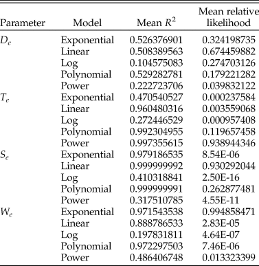

Figure 6. The four variables Te, We, De, and Se plotted as a series of bivariate plots, showing the major groups of gastropods included in this study. To aid the reader, a specimen from the extreme of each axis is illustrated as a diagram of its sagittal sections.
Closely related stromboidean families Struthiolariidae, Aporrhaidae, and Xenophoridae display commonalities in We and Se, with similar quadrate apertures that grow in size at a similar rate, but diverge in De, the rate at which they move away from the coiling axis—aporrhaid apertures remain close to the coiling axis throughout ontogeny, struthiolariids diverge more, and xenophorids diverge further and rapidly. For the specimens included here, Te is not particularly discriminatory, mostly separating Conus Linnaeus, Reference Linnaeus1758, in which the whorls almost overlap each other, from the other taxa, which all translate their apertures down to some degree. Cerithioids are dissimilar from stromboids in all parameters but Te and are united with trochoids by Se.
Struthiolariidae
The four-parameter plots for the Struthiolariidae are shown in Figure 7. There is a high degree of overlap between genera in all four parameters, but it is apparent in Figure 7 that globose specimens (Conchothyra spp., T. glomerata Darragh, Reference Darragh1991, Perissodonta spp.) are separated from fusiform specimens by We (the threshold being around 0.175 We). De ranges much wider in Tylospira than other genera. Taking the Te-We and Se-De plots and replotting them as time slices (Fig. 8), the striking similarity of younger genera appears to be convergent: the earliest genus Conchothyra Hutton, Reference Hutton1877 plots in the middle of We, Te, and De (with low-middle Se values), but the next youngest taxa (Monalaria Marwick, Reference Marwick1924 [NZ], Perissodonta Martens, Reference Martens1878 [Antarctica]) move toward the edges of the morphospace, as does the oldest species of Struthiolaria (S. calcar Hutton, Reference Hutton1885 [NZ]). Pleistocene Pelicaria vermis are quite variable in both Te and Se and overlap with both Miocene–Pleistocene Tylospira coronata and Recent Struthiolaria papulosa (Martyn, Reference Martyn1784) in Te-We space.

Figure 7. The four variables Te, We, De, and Se plotted as a series of bivariate plots for the family Struthiolariidae only. To aid the reader, a specimen from the extreme of each axis is illustrated as a diagram of its sagittal sections.

Figure 8. Time-slice diagram of struthiolariid morphology and biogeography. Shell silhouettes are approximately to scale. Paleogeographic reconstructions to the left are modified from Seton et al. (Reference Seton, Miller, Zahirovic, Gaina, Torsvik, Shephard, Talsma, Gurnis, Turner, Maus and Chandler2012). Bivariate plots shown in the center are the Te-We and Se-De panels from Fig. 7, duplicated for each time period but only plotting the specimens from that time period with older taxa grayed out. In the uppermost plot, large filled-in polygons are the convex hulls of all specimens in that species, to preserve clarity. Individual points can be seen in Fig. 7. Axes are as in Fig. 7. Lines joining specimens in the plots indicate the relationships diagrammed in the tree to the right (see also Fig. 4).
Discussion
Measuring the way snails coil has remained difficult for decades, and solutions have not been general enough to capture the astonishing morphological variety in this clade that should, in other respects, be an exemplary group for macroevolutionary studies. The aim of the present study is to provide a robust and easily implemented method that will be applicable to as wide a variety of researchers and studies as possible. The approach to the problem that we have taken allows researchers to compare the shape of regularly coiling shells with a minimum number of whorls preserved (two; to give four aperture cross sections) and without the need for external morphological landmarks that are homologous across all taxa in a given study—a severe constraint in many potential studies. The main disadvantage to our approach is that physical sectioning is destructive of specimens and CT scanning is a tool that is not yet readily available to all researchers. Despite these issues, in many cases, specimens are sufficiently numerous to allow for sectioning of some representative individuals. Another solution to this issue might be found in analyses that combine our approach with exterior landmarking to identify reliable covariation between internal and external morphological features.
Using the method presented here, workers are not constrained to a single model for all four parameters, nor are they constrained to always use the same model: it is possible to pick the best model for a group of interest. Because each available aperture contributes to the analysis, key aspects of ontogenetic development are captured. In addition, it would be possible to model different growth stages of the same snail (such as those identified by Harasewych and Petit [Reference Harasewych and Petit2013] for the land snail Extractrix Korobkov, Reference Korobkov1955).
There are limitations to the method presented here. This approach cannot deal with truly derailed coiling (coiling that is not regularly helicospiral; Seilacher and Gishlick [Reference Seilacher and Gishlick2015]), such as that exhibited by species of Stephopoma Mörch, Reference Mörch [as Moerch] and L1860 (Siliquariidae); it is only applicable to snails that coil regularly about an axis for which a sagittal section is meaningful. However, if a snail does exhibit regular coiling for any portion of its ontogeny, then this method can be used on that portion of the snail: we include in our main dataset four specimens of Tenagodus Guettard, Reference Guettard1770 (Siliquariidae; see Fig. 4) in which only the initial, “regular” whorls were digitized—these whorls exhibit similar aperture shape and similar rates of We and De to the closely related but much more regularly coiling family Turritellidae.
Shell Form and Biogeography of the Struthiolariidae
The Struthiolariidae are an ideal subject for the morphometric method presented in this paper. The oldest known member of the clade is the Cretaceous species Conchothyra parasitica, which is totally enveloped in callus. Not even the number of whorls can be discerned from the exterior of the shell, let alone any landmarks that could be used for shape analysis. Younger taxa in the clade vary between globose (Eocene Perissodonta, Miocene Tylospira) and fusiform (Neogene–Recent Struthiolaria Lamarck, Reference Lamarck1816 and Pelicaria Gray, Reference Gray1857, Recent Tylospira and Perissodonta). These taxa would be difficult or impossible to compare using a landmark-based analysis like that of Vaux et al. (Reference Vaux, Crampton, Marshall, Trewick and Morgan-Richards2017, Reference Vaux, Trewick, Crampton, Marshall, Beu, Hills and Morgan-Richards2018).
The relationships between the genera within the Struthiolariidae have been under discussion for decades (Fig. 3). It is generally agreed that Struthiolaria and Pelicaria are sister taxa (Marwick, Reference Marwick1924, Reference Marwick1951; Morton, Reference Morton1951; Zinsmeister and Camacho, Reference Zinsmeister and Camacho1980), and that Conchothyra is the oldest genus in the family and thus probably either is the progenitor of the younger taxa (Finlay and Marwick, Reference Finlay, Marwick and Finlay1937; Marwick, Reference Marwick1951; Zinsmeister, Reference Zinsmeister1976; Beu and Maxwell, Reference Beu and Maxwell1990; Stilwell, Reference Stilwell2001) or has a common ancestor with the progenitor of the younger taxa (Marwick, Reference Marwick1924; Zinsmeister and Camacho, Reference Zinsmeister and Camacho1980). Stilwell (Reference Stilwell2001), in a detailed treatment, showed that Monalaria originated from a small species of Conchothyra, C. marshalli (Trechmann, Reference Trechmann1917), and further connected the origins of Struthiolarella Steinmann and Wilckens, Reference Steinmann and Wilckens1908 and Antarctodarwinella Zinsmeister, Reference Zinsmeister1976 (both now referred to Perissodonta by Beu [Reference Beu2009]) to Conchothyra. Struthiolaria either originates from Monalaria (Marwick Reference Marwick1924) or Conchothyra (the gap in their stratigraphic distributions being explained by either a period of restriction to deep water, for which rock has not been preserved, or evolution outside the New Zealand region, according to Beu and Maxwell [Reference Beu and Maxwell1990]). However, Monalaria concinna (Suter, Reference Suter1917) and Struthiolaria calcar are much closer in De and We (distance of aperture to coiling axis and whorl expansion) (Fig. 6) than S. calcar is to either species of Conchothyra.
Previous hypotheses of the relationships between genera in this family have centered on the nature of the external morphology, such as the curvature of the columella, the sinuosity of the outer lip (measured approximately perpendicular to the terminal aperture shape measured here and thus not exerting a strong influence on the Se parameter), and particularly the nature of the callus and sculpture (e.g., Zinsmeister and Camacho Reference Zinsmeister and Camacho1980; Beu and Maxwell Reference Beu and Maxwell1990; Darragh Reference Darragh1991). However, despite its strikingly “extreme” external morphology, C. parasitica does not plot at the extreme of any of the three coiling parameters De, Te or We. Obviously, in the absence of molecular data, asserting that any given morphological character is a truer representation of relationship than another is pure conjecture, but the extent of callus particularly is known to be labile in both struthiolariids and the related strombids, whereas, as we show here (Figs. 7, 8), two or three of the De, Te, and We parameters are consistent within any given clade.
The final living genus, Tylospira, with only a single extant species in Australia, is the most interesting taxon in terms of phylogenetic placement. Darragh (Reference Darragh1991) postulated Monalaria as the ancestral taxon to Tylospira and suggested that the strong similarities (in form and sculpture) between the earliest Tylospira, T. glomerata, and the Eocene species of Perissodonta (then described as Antarctodarwinella) are the result of convergence, instead placing Tylospira closer to Monalaria because of similarities in whorl-profile shape and sculpture between Monalaria and two younger species of Tylospira, T. clathrata (Tate, Reference Tate1885) and T. coronata. However, we suggest here that, in fact, it is equally likely that Tylospira was derived from Perissodonta after the opening of the Drake Passage and the initiation of the Antarctic Circumpolar Current (ACC). In shell-form parameters, T. glomerata is almost indistinguishable from Perissodonta nordenskjoldi (Wilckens, Reference Wilckens1911), and furthermore, given the prevailing current directions in the Tasman Sea are eastward, westward dispersal from New Zealand to Australia is unlikely, but transport of mollusks eastward around the ACC has been documented (Beu et al. Reference Beu, Griffin and Maxwell1997; Gordillo Reference Gordillo2006)—largely in the context of dispersal events between New Zealand and South America, but if transport is possible between South America and New Zealand, then it seems plausible that it could also occur between South America and Australia. Resemblances between younger species of Tylospira and the New Zealand struthiolariid lineage, particularly Pelicaria (which was once considered congeneric with T. scutulata) are then convergent. It is worth noting that Pelicaria and those species of Tylospira for which the protoconch are known are both direct developers, unlike the rest of their confamilials, which are planktotrophs.
Combining rate and shape parameters (Fig. 8) with reconstructions of the Southern Hemisphere at the time periods for which we have specimens, we suggest that in the Paleogene, the genera included here split into two lineages—a New Zealand endemic lineage, comprising Conchothyra, Monalaria, Struthiolaria, and Pelicaria, and a circum-Antarctic lineage, comprising Perissodonta, also derived from Conchothyra stock and arriving in South America by the Paleogene, and Tylospira, derived from Perissodonta and arriving in Australia after the opening of Drake Passage in the Miocene. This relationship of Tylospira to Perissodonta, aside from a brief discussion and rejection by Darragh (Reference Darragh1991), has not to our knowledge been postulated before.
The New Zealand endemics (Monalaria, Struthiolaria, Pelicaria), initially reduce their whorl expansion, develop more quadrate apertures, and slightly increase their rate of translation compared with C. parasitica. Neogene and Recent members of this group occupy a wide swath of the We-Te morphospace, but never regain the “globose” region of high-We and high-Te observed for Conchothyra; they occupy almost the entire range of Se but only low De regions of the Se-De morphospace.
The circum-Antarctic lineage, comprising Perissodonta and Tylospira, initially retains the globose form of Conchothyra parasitica and increases the rate of whorl expansion and of aperture distance from the coiling axis, reduces the rate of translation, and becomes more quadrate in aperture shape. However, post-Miocene, the Tylospira lineage converges toward the same area of We-Te morphospace as the Struthiolaria+Pelicaria lineage, but with a narrower range of shapes and a much wider range of De values. We only had access to one specimen of Recent T. scutulata, and we were unable to get access to specimens of the rare extant species of Perissodonta (P. mirabilis [E. A. Smith, Reference Smith1875] and P. georgiana Strebel, Reference Strebel1908) but note that all three of these species are much more fusiform than their ancestors, following this trend.
Obviously, a lack of specimens of the older taxa precludes firm conclusions from being drawn here, but the results shown invite further research and illustrate the utility of spiral morphometrics for analyses of clades for which species vary between having few external features (e.g., Conchothyra parasitica) or many (e.g., Tylospira coronata).
Conclusions
The spiral Gastropoda are one of the most speciose and disparate of animal groups but have been a challenge to analyze using morphometric techniques, despite discussion of the issue by many authors. In this paper, we provide a methodology involving simple data-capture techniques that can be used to model the growth-rate parameters and aperture shapes that describe overall gastropod form.
The advantages of the method presented here are that it allows comparison of shells that lack sculptural homologies, have a variable number of whorls, or have very disparate exterior shapes. We illustrate this by applying the method to a pilot dataset of species from the austral family Struthiolariidae and find evidence to support a previously discarded hypothesis of relationship between Perissodonta and Tylospira that is congruent with the distribution of these genera in both space and time.
We provide a transparent methodology with code written in the open-source language R to allow workers to reproduce our empirically derived morphospace on any set of snails that they choose.
Data Availability Statement
Data available from the Dryad Digital Repository: https://doi.org/10.5061/dryad.p5hqbzknw.
Museum and sectioning information for all specimens used in this study can be found in Supplementary Table 1 (“S_Table_1_Specimens.csv”), metadata for analyses in Supplementary Table 2 (“S_Table_2_metadata.csv”), and Hangle shape data as Supplementary Table 3 (“S_Table_3_hangle_output.csv). Code to perform analyses is available as Supplementary File 1 (“S_File_1_Process_Snails.Rmd”) and Supplementary File 2 (“S_File_2_Struthiolariidae.Rmd”). Images and landmark data are available on Dryad at https://doi.org/10.5061/dryad.p5hqbzknw. Analyses are performed using R base packages (R Core Team 2020) plus dplyr (Wickham et al. Reference Wickham, François, Henry and Müller2020), magrittr (Bache and Wickham Reference Bache and Wickham2014), stringr (Wickham Reference Wickham2019), data.table (Dowle and Srinivasan Reference Dowle and Srinivasan2019), ggplot2 (Wickham Reference Wickham2016), reshape2 (Wickham Reference Wickham2007), scatterplot3d (Ligges and Mächler Reference Ligges and Mächler2003), DT (Xie et al. Reference Xie, Cheng and Tan2020), threejs (Lewis Reference Lewis2020), gridExtra (Auguie Reference Auguie2017), jpeg (Urbanek Reference Urbanek2019), pander (Daróczi and Tsegelskyi Reference Daróczi and Tsegelskyi2018), magick (Ooms Reference Ooms2020), plot3D (Soetaert Reference Soetaert2019), and other packages from tidyverse (Wickham et al. Reference Wickham, Averick, Bryan, Chang, McGowan, François, Grolemund, Hayes, Henry, Hester, Kuhn, Pedersen, Miller, Bache, Müller, Ooms, Robinson, Seidel, Spinu, Takahashi, Vaughan, Wilke, Woo and Yutani2019).
Acknowledgments
CT scanning was performed at the Australian Synchrotron's Imaging and Medial Beamline (IMBL), session 2014/3, experiment M8599. The authors are indebted to the staff at the Australian Synchrotron and the museum curators and researchers who kindly made specimens available for sectioning and scanning, sometimes at very short notice, J. Simes, M. Terezow, and A. Beu at GNS Science and R. Schmidt and T. Darragh at Museum Victoria. E. G. C. Smith provided invaluable mathematical and coding advice and originally suggested the title. We would also like to thank the members of the Jablonski and Price labs at the University of Chicago for useful discussions on snail morphometrics, and S. Edie (CalTech) for his comments on the article. P. D. Polly, P. Wagner, and an anonymous referee provided comments in review which improved the article greatly.


