Introduction
The late Pleistocene extinction is one of the largest extinction events in North America in the past 55 Myr (Alroy Reference Alroy, MacPhee and Sues1999), and it is particularly notable because of the role it had in shaping current biodiversity patterns (Koch and Barnosky Reference Koch and Barnosky2006; Hofreiter and Stewart Reference Hofreiter and Stewart2009; Smith et al. Reference Smith, Tomé, Elliot Smith, Lyons, Newsome and Stafford2016). Mammals were among the most adversely affected groups, and it is estimated that more than 30 genera disappeared from the continent (Grayson Reference Grayson1991, Reference Grayson2007; Koch and Barnosky Reference Koch and Barnosky2006; Faith and Surovell Reference Faith and Surovell2009; Meltzer Reference Meltzer2015; Stuart Reference Stuart2015). The causes of the extinction have been extensively debated, and several extinction models have been proposed. Some models identify climate change as the primary causal factor (e.g., Graham and Lundelius Reference Graham, Lundelius, Martin and Klein1984; Guthrie Reference Guthrie, Martin and Klein1984; Kiltie Reference Kiltie, Martin and Klein1984; King and Saunders Reference King, Saunders, Martin and Klein1984; Barnosky Reference Barnosky1986; Ficcarelli et al. Reference Ficcarelli, Coltorti, Moreno-Espinosa, Pieruccini, Rook and Torre2003; Forster Reference Forster2004; Scott Reference Scott2010; Cooper et al. Reference Cooper, Turney, Hughen, Brook, McDonald and Bradshaw2015), others point to overhunting and alteration of ecosystems by early human populations (Martin Reference Martin, Martin and Wright1967, Reference Martin, Martin and Klein1984; Mosimann and Martin Reference Mosimann and Martin1975; Diamond Reference Diamond1989; Fisher Reference Fisher and Haynes2009; Ripple and Van Valkenburgh Reference Ripple and Van Valkenburgh2010), and yet others point to a combination of climate change and human impacts (e.g., Koch and Barnosky Reference Koch and Barnosky2006; Emery-Wetherell et al. Reference Emery-Wetherell, McHorse and Davis2017). Another set of extinction models invoke catastrophic events, such as a bolide impact (Firestone et al. Reference Firestone, West, Kennett, Becker, Bunch, Revay and Schulz2007) or a hyperdisease (MacPhee and Marx Reference MacPhee, Marx, Goodman and Patterson1997).
Currently there is little support for the catastrophic extinction models (e.g., Lyons et al. Reference Lyons, Smitha and Brown2004; Koch and Barnosky Reference Koch and Barnosky2006; Surovell et al. Reference Surovell, Holliday, Gingerich, Kreton, Haynes, Hilman, Wagner, Johnson and Claeys2009; Holliday et al. Reference Holliday, Surovell, Meltzer, Grayson and Boslough2014; Meltzer et al. Reference Meltzer, Holliday, Cannon and Miller2014), and much of the debate regarding the late Pleistocene extinctions is focused on the relative importance of climate change versus human impacts, particularly hunting. Some of the climate change extinction models point to nutritional stress as the primary factor responsible for the extinctions (e.g., Graham and Lundelius Reference Graham, Lundelius, Martin and Klein1984; Guthrie Reference Guthrie, Martin and Klein1984). The recent development of different methodologies for the reconstruction of mammalian paleodiets (e.g., dental wear and stable isotopes) may shed new light on this matter by allowing the formulation and testing of novel hypotheses about patterns of feeding ecology expected under different extinction models.
Here, we employ methodologies based on dental wear (i.e., mesowear and low-magnification dental microwear) to study dietary patterns of horses and bison from three geographic areas of North America. We use those data to evaluate two nutritionally based extinction models relating to climate-induced vegetation changes during the terminal Pleistocene: the coevolutionary disequilibrium (Graham and Lundelius Reference Graham, Lundelius, Martin and Klein1984) and mosaic-nutrient extinction models (Guthrie Reference Guthrie, Martin and Klein1984). We also examine the prevalence of enamel hypoplasia in the samples of horse and bison as a proxy for the incidence of early systemic stress in these ungulates during the late Pleistocene. In the context of the late Pleistocene extinctions, the study of enamel hypoplasia provides the opportunity to test whether herbivorous mammals were potentially experiencing increased levels of systemic stress during the terminal Pleistocene, as predicted by the coevolutionary disequilibrium and mosaic-nutrient models as well as other climate-based extinction models. We emphasize that a comprehensive test of both models would require comparing changes in dental wear and enamel hypoplasia during earlier glacial–interglacial transitions as well as during the terminal Pleistocene. However, the temporal resolution needed to undertake such a study is presently lacking for previous glacial–interglacial transitions. Therefore, the objective of the present study is to evaluate the consistency of the data on dental wear and enamel hypoplasia collected for North American late Pleistocene horses and bison with respect to predictions established for the coevolutionary disequilibrium and mosaic-nutrient models.
We chose horses and bison for this study because they were relatively abundant in North American, late Pleistocene landscapes and are well represented in the fossil record of that continent (Faunmap Working Group 1994; Grayson Reference Grayson2016). In addition, some studies suggest that these ungulate mammals may have interacted ecologically as competitors for food resources (e.g., Feranec et al. Reference Feranec, Hadly and Paytan2009).
The Coevolutionary Disequilibrium Extinction Model
The coevolutionary disequilibrium extinction model assumes that late Pleistocene communities were highly coevolved systems, similar to those currently found on the African savannas (Graham and Lundelius Reference Graham, Lundelius, Martin and Klein1984). The present-day African grazing succession is an example of a coevolved system in which grazing by one mammalian herbivore species stimulates the growth of plant species or plant parts that in turn form the food resource of another herbivore species. In this ecosystem, coevolved foraging sequences partition the environment through well-defined niche differentiation, allowing the coexistence of many large herbivores (e.g., Gwynne and Bell Reference Gwynne and Bell1968; Bell Reference Bell1971; Murray and Brown Reference Murray and Brown1993).
Paleontological evidence suggests that organisms responded individualistically to the climatic changes at the end of the Pleistocene (e.g., Graham et al. Reference Graham, Lundelius, Graham, Schroeder, Toomey, Anderson and Barnosky1996; Stewart Reference Stewart2009). The coevolutionary disequilibrium model proposes that the individualistic response of plant species during this time interval resulted in large-scale restructuring of vegetation, causing a disruption of coevolutionary interactions between plants and animals (Graham and Lundelius Reference Graham, Lundelius, Martin and Klein1984). These changes are postulated to have reduced niche differentiation among large herbivorous mammals, leading to competition for dietary resources and causing nutritional stress in some species. Competition may have driven species with reduced fitness to extinction, whereas species better adapted to the new community patterns would have thrived and established a new interaction sphere (Graham and Lundelius Reference Graham, Lundelius, Martin and Klein1984).
Testable assumptions/predictions of the coevolutionary disequilibrium model include chronological congruence of plant community changes and animal extinctions, the occurrence of relictual populations of animals and plants in association with one another, and divergence and habitat partitioning of surviving large herbivores as a consequence of competition (Graham and Lundelius Reference Graham, Lundelius, Martin and Klein1984). Using newer analytical techniques, we can now expand the testing of assumptions of the coevolutionary disequilibrium model. Specifically, evaluation of mesowear and low-magnification microwear permits testing of well-defined niche differentiation and potential resource competition in large ungulates both before and after the onset of major environmental changes at the terminal Pleistocene as follows:
H10: Before rapid climatic changes at the end of the Pleistocene, sympatric species of horse and bison inhabiting North America did not differ significantly in their diets, suggesting that they did not partition the available food resources.
H1A: Before rapid climatic changes at the end of the Pleistocene, sympatric species of horse and bison differed significantly in their diets, indicating that they partitioned the available food resources.
H1 prediction: If sympatric species of horse and bison partitioned food resources before the rapid climatic changes of the postglacial (i.e., during the preglacial and full-glacial time intervals), then the signals of the dietary proxies (mesowear and low-magnification microwear, in this study) should be statistically different for horse and bison.
H20: During the postglacial, sympatric species of horse and bison did not differ significantly in their diets, suggesting that they were not partitioning the available food resources and were potentially competing for them.
H2A: During the postglacial, sympatric species of horse and bison from this time interval differed significantly in their diets, indicating that they were partitioning the available food resources.
H2 prediction: If sympatric species of horse and bison were not partitioning available food resources during the postglacial, as would be consistent with the assumptions of coevolutionary disequilibrium, then the signal of each dietary proxy (i.e., dental microwear and mesowear) should not be significantly different for horse and bison.
The Mosaic-Nutrient Extinction Model
Like the coevolutionary disequilibrium model, the mosaic-nutrient model for extinction focuses on an altered vegetational landscape as a primary driver of terminal Pleistocene extinctions. This model assumes that before the terminal Pleistocene, a mosaic vegetation pattern was present and allowed ungulates, especially large caecalid ungulates (e.g., horse and mammoth), to obtain a proper mix of nutrients needed for survival (Guthrie Reference Guthrie, Martin and Klein1984). Unlike caecalid ungulates, ruminants (e.g., bison and deer) are able to synthesize some essential nutrients in the rumen through the help of microbial activity (Guthrie Reference Guthrie, Martin and Klein1984). In addition, ungulates are adapted to overcome some plant defenses but not others. For example, large caecalid grazers like horse and mammoth have dental and digestive physiological adaptations to deal with grass phytoliths and a high concentration of fiber (Janis Reference Janis1976, Reference Janis, Russell, Santoro and Sigogneau-Russell1988), but are not as efficient at detoxifying allelochemics, which are commonly found in forbs and other browse, as is the case for ruminants (Janis Reference Janis1976; Guthrie Reference Guthrie, Martin and Klein1984). Therefore, as long as a diversity of plant species were available, large caecalids may have acquired a proper mix of nutrients by diluting a variety of different toxins, which could be detoxified in reduced quantities (Guthrie Reference Guthrie, Martin and Klein1984).
The mosaic-nutrient model proposes that at the end of the Pleistocene, changes in seasonal climatic regimes (i.e., increased seasonality and less intra-annual variability) led to decreased local plant diversity and increased zonation of plant communities and resulted in a shift in net anti-herbivore defenses (Guthrie Reference Guthrie, Martin and Klein1984). Collectively, those changes may have differentially impacted the ability of some herbivores (e.g., caecalid ungulates) to effectively obtain nutrients because of limitations in digestive physiology (Guthrie Reference Guthrie, Martin and Klein1984).
As with the coevolutionary disequilibrium model, newer analytical techniques permit direct testing for dietary change that may support or refute the mosaic-nutrient model. Specifically, evaluation of mesowear and low-magnification microwear permits testing of changes in the variety of food resources consumed by megafauna both before and at the terminal Pleistocene as follows:
H30: Bison and horse species did not suffer a decrease in the variety of plant species consumed during the postglacial relative to preglacial and full-glacial periods.
H3A: Bison and horse species underwent a significant decrease in the variety of plants consumed during the postglacial, potentially due to a reduction in local plant diversity.
H3 prediction: If species of horse and bison experienced a significant decrease in the variety of plants in their diets during the postglacial, then the statistical dispersion (measured by the variance) of the variables of each dietary proxy (i.e., low-magnification microwear variables and mesowear score) should be significantly smaller for this time interval than for the preglacial and full-glacial periods.
A Test for Both Models: Systemic Stress and Enamel Hypoplasia
Both the coevolutionary disequilibrium and mosaic-nutrient extinction models point to systemic stress, particularly nutritional stress, on herbivorous mammals as one of the primary factors responsible for the late Pleistocene extinctions (Graham and Lundelius Reference Graham, Lundelius, Martin and Klein1984; Guthrie Reference Guthrie, Martin and Klein1984). This would trigger a “bottom-up” ecosystem collapse starting with the herbivores and filtering upward to the apex carnivores. For either extinction model to be considered feasible, not only do the formulated predictions have to be met, but also the occurrence of broad systemic stress in herbivores during the terminal Pleistocene must be demonstrated. Recent advances regarding the inference of physiological stress from dental remains permit testing of this hypothesis.
Periods of disruption in tooth development correlated with systemic stress during enamel matrix formation are recorded in the teeth in the form of tooth defects known as enamel hypoplasia (Goodman and Rose Reference Goodman and Rose1990; Moggi-Cecchi and Crovella Reference Moggi-Cecchi and Crovella1991; Hillson Reference Hillson1996, Reference Hillson2005; Kierdorf and Kierdorf Reference Kierdorf and Kierdorf1997; Guatelli-Steinberg Reference Guatelli-Steinberg2000, Reference Guatelli-Steinberg2003; Witzel et al. Reference Witzel, Kierdorf, Schultz and Kierdorf2008). These tooth defects have been extensively used in anthropological and archaeological studies to infer the health of past and present primate populations, including humans (e.g., Goodman and Rose Reference Goodman and Rose1990; Moggi-Cecchi and Crovella Reference Moggi-Cecchi and Crovella1991; Skinner and Goodman Reference Skinner, Goodman, Saunders and Katzenberg1992; Hillson Reference Hillson1996, Reference Hillson2005; Guatelli-Steinberg Reference Guatelli-Steinberg1998, Reference Guatelli-Steinberg2000, Reference Guatelli-Steinberg2003; Lukacs Reference Lukacs2001, Reference Lukacs2009; Skinner and Hopwood Reference Skinner and Hopwood2004; King et al. Reference King, Humphrey and Hillson2005; Schwartz et al. Reference Schwartz, Reid, Dean and Zihlman2006; Witzel et al. Reference Witzel, Kierdorf, Schultz and Kierdorf2008; Guatelli-Steinberg et al. Reference Guatelli-Steinberg, Ferrell and Spence2012; Smith and Boesch Reference Smith and Boesch2015). In contrast, fewer studies have been conducted on archaeological and paleontological non-primate mammals, including Neogene rhinoceroses (Mead Reference Mead1999; Roohi et al. Reference Roohi, Raza, Khan, Ahmad and Akhtar2015), domestic pigs and wild boar (Dobney and Ervynck Reference Dobney and Ervynck2000; Dobney et al. Reference Dobney, Ervynck, Albarella and Rowley-Conwy2004; Witzel et al. Reference Witzel, Kierdorf, Dobney, Ervynck, Vanpoucke and Kierdorf2006), late Pleistocene and Holocene bison (Niven Reference Niven2002; Niven et al. Reference Niven, Egeland and Todd2004; Byerly Reference Byerly2007), Pliocene giraffids (Franz-Odendaal et al. Reference Franz-Odendaal, Chinsamy and Lee-Thorp2004), cattle (Kierdorf et al. Reference Kierdorf, Zeiler and Kierdorf2006), Pleistocene equids (Timperley and Lundelius Reference Timperley and Lundelius2008), domestic sheep and goats (Kierdorf et al. Reference Kierdorf, Witzel, Upex, Dobney and Kierdorf2012; Upex et al. Reference Upex, Balasse, Tresset, Arbuckle and Dobney2014), and the Pleistocene notungulate Toxodon (Braunn et al. Reference Braunn, Ribeiro and Ferigolo2014).
The Federation Dentaire Internationale (FDI) established an international index for the study of enamel hypoplasia that recognizes different categories of this defect: single pits, areas missing enamel, nonlinear grooves, nonlinear multiple pits, horizontal linear grooves, and horizontal linear pits (FDI 1982). Nonlinear pits and areas missing enamel are thought to result from localized physical trauma, usually associated with a thinning of the bone covering the developing tooth commonly caused by poor maternal diet (deficiencies in calcium, vitamin A, or vitamin D) and premature births (Skinner and Hung Reference Skinner and Hung1986). Small horizontal linear pits and horizontal linear grooves are known as linear enamel hypoplasia. Linear defects have been associated with different systemic stressors (e.g., weaning, parturition, nutritional stress, and illness) at the time of tooth formation (Franz-Odendaal Reference Franz-Odendaal2004; Franz-Odendaal et al. Reference Franz-Odendaal, Chinsamy and Lee-Thorp2004). Some researchers consider that the width and depth of linear enamel hypoplasia correspond, respectively, to the duration of the stress episode and its severity (Goodman et al. Reference Goodman, Armelagos and Rose1980; Suckling Reference Suckling1989).
In this study, we examined the prevalence of enamel hypoplasia in the cheek teeth of North American late Pleistocene equids and bison as a proxy for the incidence of early systemic stress. The hypotheses tested are:
H40: Horse and bison do not show a significant difference in the frequency of enamel hypoplasia and number of hypoplastic events per affected tooth during the terminal Pleistocene (postglacial) relative to previous time intervals.
H4A: Horses, in contrast to bison, show a significant increase in the frequency of enamel hypoplasia and number of hypoplastic events per affected tooth during the terminal Pleistocene (postglacial), potentially caused by an increase in systemic stress (specifically nutritional stress) due to new vegetational associations.
H4 prediction: The coevolutionary disequilibrium and mosaic-nutrient extinction models both predict an increase in systemic stress (specifically nutritional stress), particularly for the species that became extinct. Systemic stress encountered by an individual while the dentition was being formed can be inferred by examining for enamel hypoplasia. If horses experienced an important increase in systemic stress during the postglacial, the frequency of enamel hypoplasia and the number of hypoplastic events per affected tooth for this time interval should be significantly greater than those for earlier time periods (full-glacial and preglacial).
Materials and Methods
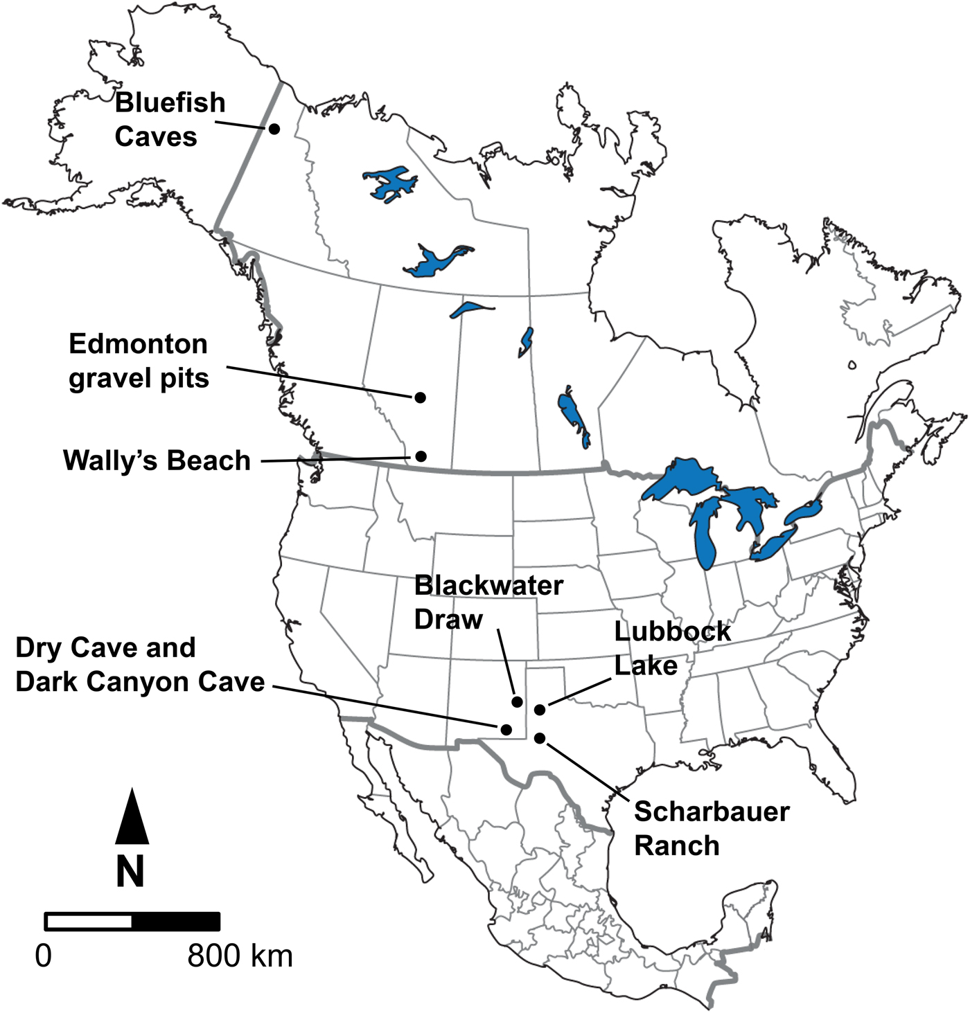
The samples for study consisted of late Pleistocene equid and bison cheek teeth (both isolated as well as from skulls and mandibles) from Bluefish Caves, Yukon Territory; the Edmonton area gravel pits and Wally's Beach site, Alberta; and several sites in the American Southwest, including Dark Canyon Cave, Dry Cave, and Blackwater Draw, New Mexico, as well as Sharbauer Ranch and Lubbock Lake sites, Texas (Fig. 1). These sites were selected for study because they are primarily arranged in a north–south transect along the Western Interior of North America, allowing us to evaluate responses in diet and systemic stress of horses and bison at different latitudes. All of the specimens we studied are deposited in the following institutions, with corresponding institutional acronyms and geographic location indicated in parentheses: Archaeology Collection (Bluefish Caves; MgVo-1, 2, and 3) of the Canadian Museum of History (CMH; Gatineau, Quebec, Canada); Quaternary Paleontology (P) and Archaeology collections (Wally's Beach site; DhPg-8) of the Royal Alberta Museum (RAM; Edmonton, Alberta, Canada); Vertebrate Paleobiology Collection, Laboratory for Environmental Biology, University of Texas at El Paso (UTEP; El Paso, Texas, USA); and the Vertebrate Paleontology collection of the Vertebrate Paleontology Laboratory, Jackson School Museum of Earth History, University of Texas at Austin (TMM; Austin, Texas, USA).

Figure 1. Geographic location of the fossil sites considered in this study.
The horse and bison teeth were identified using different published sources. Species identification was based on the studies by Lundelius (Reference Lundelius and Hester1972), Jass et al. (Reference Jass, Burns and Milot2011), and Harris (Reference Harris2015) for the bison teeth and Barrón-Ortiz et al. (Reference Barrón-Ortiz, Rodrigues, Theodor, Kooyman, Yang and Speller2017) for the equid teeth. Bison antiquus was identified for the American Southwest sample and Bison sp. for the sample from Alberta. We identified two equid species, caballine and non-caballine, for the American Southwest, but only the caballine species was identified in the samples from Alberta and the Yukon Territory. Given the state of flux in equid taxonomy, we refer to the caballine species as Equus “ferus” and to the non-caballine species as “Equus conversidens,” to acknowledge that the nomenclature may change with additional taxonomic studies. Following a proposal by Gentry et al. (Reference Gentry, Clutton-Brock and Groves1996), the International Commission on Zoological Nomenclature has ruled that the names for some wild forms have precedence over those for domestic forms, if these are considered conspecific (ICZN 2003; Gentry et al. Reference Gentry, Clutton-Brock and Groves2004). Therefore, Equus ferus Boddaert, Reference Boddaert1785 has precedence over Equus caballus Linnaeus, Reference Linnaeus1758; however, this has not been consistently followed in the literature (Wilson and Reeder Reference Wilson and Reeder2005). Equus conversidens is considered a valid taxon in some studies (e.g., Scott Reference Scott, Reynolds and Reynolds1996; Azzaroli Reference Azzaroli1998; Bravo-Cuevas et al. Reference Bravo-Cuevas, Jiménez-Hidalgo and Priego-Vargas2011; Priego-Vargas et al. Reference Priego-Vargas, Bravo-Cuevas and Jiménez-Hidalgo2017) and a nomen dubium in other studies (e.g., Winans Reference Winans1985, Reference Winans, Prothero and Schoch1989; Heintzman et al. Reference Heintzman, Zazula, MacPhee, Scott, Cahill, McHorse and Kapp2017). The generic name Haringtonhippus was recently proposed for the non-caballine horse (Heintzman et al. Reference Heintzman, Zazula, MacPhee, Scott, Cahill, McHorse and Kapp2017). However, a recent phylogenetic analysis identified Haringtonhippus within the group that includes species traditionally assigned to Equus (Barrón-Ortiz et al. Reference Barrón-Ortiz, Jass and Bravo-Cuevas2018). Regardless of how the caballine and non-caballine species are named, several studies consistently identify them as distinct lineages (e.g., Weinstock et al. Reference Weinstock, Willerslev, Sher, Tong, Ho, Rubenstein and Storer2005; Barrón-Ortiz et al. Reference Barrón-Ortiz, Rodrigues, Theodor, Kooyman, Yang and Speller2017; Heintzman et al. Reference Heintzman, Zazula, MacPhee, Scott, Cahill, McHorse and Kapp2017); therefore, their recognition as separate taxonomic units in the present study is well supported.
The data we collected were arranged into preglacial, full-glacial, and postglacial time intervals. The material from Bluefish Caves, which consisted of only one equid species (E. “ferus”), could only be divided into two time intervals: preglacial/full-glacial (~31– 14 kyr RCBP [radiocarbon years before the present]) and postglacial (~14–10 kyr RCBP) (Table 1). Specimens were assigned to one of these two time intervals based on published work (Cinq-Mars Reference Cinq-Mars1979; Morlan Reference Morlan1989), documents on file at the CMH (CMH Archives A2002-9 [Jacques Cinq-Mars's documents]: box 11, f.7), and the spatial and stratigraphic provenance of equid specimens (retrieved from specimen catalogs and maps in the CMH Archives; A2002-9: box 2, f.1, f.2, f.4; box 3, f.1, f.3 – f.9, f.13; box 8, f.4, f.5) relative to directly radiocarbon-dated bones (Canadian Archaeological Radiocarbon Database [CARD 2.0]). These divisions correspond to a change in the vegetation of the region from tundra during the preglacial/full-glacial to dwarf birch during the postglacial (Cinq-Mars Reference Cinq-Mars1979; Ritchie et al. Reference Ritchie, Cinq-Mars and Cwynar1982). Different publications mention the occurrence of bison remains at Bluefish Caves (Cinq-Mars Reference Cinq-Mars1979, Reference Cinq-Mars1990), but we were unable to locate any bison cheek teeth in the collection of the CMH. Thus, we only studied equid specimens from this site.
Table 1. Temporal distribution of the late Pleistocene equid and bison samples studied. Post-LGM = postglacial; LGM = full-glacial; Pre-LGM = preglacial. An asterisk (*) indicates the sample spans Pre-LGM and LGM time intervals.

The samples from Alberta were divided into preglacial (>60–21 kyr RCBP) and postglacial time intervals (~13– 0 kyr RCBP) (Table 1) based on published radiocarbon dates (Waters et al. Reference Waters, Stafford, Kooyman and Hills2015) and the association of specimens with localities that have only yielded dates of preglacial or postglacial age (Burns Reference Burns1996; Jass et al. Reference Jass, Burns and Milot2011). Fossil material from the full-glacial is not represented in Alberta, because most of the province was covered by the Laurentide and Cordilleran ice sheets at that time (Young et al. Reference Young, Burns, Smith, Arnold and Rains1994, Reference Young, Burns, Rains and Schowalter1999; Burns Reference Burns1996; Jass et al. Reference Jass, Burns and Milot2011). The specimens from Alberta consisted of only one equid species (E. “ferus”; although a second less common species, “E. conversidens,” is recognized from the Edmonton area gravel pits [Barrón-Ortiz et al. Reference Barrón-Ortiz, Rodrigues, Theodor, Kooyman, Yang and Speller2017]) and material referable to Bison sp.
The fossil material from the American Southwest (specifically eastern New Mexico and western Texas) was divided into preglacial (~25–20 kyr RCBP), full-glacial (~20–15 kyr RCBP), and postglacial (~15–10 kyr RCBP) ages (Harris Reference Harris1987, Reference Harris1989, Reference Harris2015; Tebedge Reference Tebedge1988; Haynes Reference Haynes1995; Holliday and Meltzer Reference Holliday and Meltzer1996) (Table 1). We were able to obtain data for only one equid species (“E. conversidens”) during the preglacial, whereas for the full-glacial we were able to collect data for two equid species (E. “ferus” and “E. conversidens”). We also collected data for postglacial specimens of E. “ferus” and “E. conversidens.” For B. antiquus, only specimens from postglacial localities showed a state of preservation that allowed us to study dental wear and enamel hypoplasia; therefore, the analyses for this species were limited to this time interval. The sampling limitations for these and all other localities studied were imposed by the preservation of the specimens and their availability at the repository institutions.
Analysis of Dental Wear
We used the extended mesowear (Franz-Odendaal and Kaiser Reference Franz-Odendaal and Kaiser2003; Kaiser and Solounias Reference Kaiser and Solounias2003) and low-magnification microwear methods (Solounias and Semprebon Reference Solounias and Semprebon2002; following the modifications by Fraser et al. [2009]), to test the outlined hypotheses for the coevolutionary disequilibrium and mosaic-nutrient extinction models. A total of 122 specimens for the dental microwear analysis and 102 specimens for the mesowear analysis were studied, consisting mostly of isolated teeth (Supplementary Tables 1 and 2).
Low-Magnification Microwear
Low-magnification microwear and microwear texture analysis are currently the most widely applied methodologies for the study of dental microwear (e.g., Solounias and Semprebon Reference Solounias and Semprebon2002; Ungar et al. Reference Ungar, Brown, Bergstrom and Walker2003, Reference Ungar, Scott, Grine and Teaford2010; Scott et al. Reference Scott, Ungar, Bergstrom, Brown, Grine, Teaford and Walker2005, Reference Scott, Ungar, Bergstrom, Brown, Childs, Teaford and Walker2006; Semprebon et al. Reference Semprebon, Godfrey, Solounias, Sutherland and Jungers2004; Merceron et al. Reference Merceron, Blondel, Brunet, Sen, Solounias, Viriot and Heintz2004, Reference Merceron, Blondel, de Bonis, Koufos and Viriot2005, Reference Merceron, Escarguel, Angibault and Verheyden-Tixier2010; Nelson et al. Reference Nelson, Badgley and Zakem2005; Gomes Rodrigues et al. Reference Gomes Rodrigues, Merceron and Viriot2009). In this study, we examined dental microwear at a low magnification (35×) using high-resolution clear-epoxy casts. We counted microwear features on high dynamic range images (HDR; Fig. 2) prepared following the methodology in Fraser et al. (Reference Fraser, Mallon, Furr and Theodor2009), using an Olympus E-M10 digital camera and a Nikon SMZ1500 stereomicroscope; the digital resolution of the images obtained is 0.6 pixels/μm. Cleaning, molding, and casting of the teeth studied were done according to Solounias and Semprebon (Reference Solounias and Semprebon2002). Only teeth in middle stages of wear were used. To minimize systematic biases during data collection, we randomized the order of the specimens during photography and the order of the HDR images was also randomized before data collection to ensure observer blindness (Mihlbachler et al. Reference Mihlbachler, Beatty, Caldera-Siu, Chan and Lee2012). All counts were done by the same researcher (C.I.B.-O.).
Figure 2. High dynamic range image of the paracone lingual enamel band of an equid tooth (upper right M1; UTEP 22-1609) showing one of the 0.4 × 0.4 mm counting areas and the microwear features evaluated in this study. Abbreviations: crs = cross scratch; cs = coarse scratch; fs = fine scratch; g = gouge; lp = large pit; p = small pit.
The majority of the specimens we studied consisted of isolated upper (M1–M3) and lower (m1–m3) molars. Previous studies of low-magnification dental microwear have identified that homologous upper and lower teeth show comparable dental microwear features (Merceron et al. Reference Merceron, Blondel, Brunet, Sen, Solounias, Viriot and Heintz2004; Semprebon et al. Reference Semprebon, Godfrey, Solounias, Sutherland and Jungers2004); therefore, upper and lower molars were not studied separately. In the case of teeth belonging to the same individual, we studied the second molar, and if this tooth was damaged or absent we selected at random one of the other associated molars that were well-preserved. We preferentially studied microwear features on the lingual enamel band of the paracone and/or metacone for the upper molars and the lingual enamel band of the protoconid and/or hypoconid for the lower molars. For specimens in which these enamel bands were damaged, we collected microwear data from the lingual enamel band of the fossettes for the upper molars and the buccal enamel band of the protoconid and/or hypoconid for the lower molars.
The microwear variables scored per tooth specimen are partially based on those presented by Solounias and Semprebon (Reference Solounias and Semprebon2002) and include the average number of scratches and pits per two counting areas on the enamel band, each 0.4 × 0.4 mm. Pits are microwear features that are circular to subcircular in outline with a length to width ratio of less than 4:1, whereas scratches are elongated features, typically with a length to width ratio of at least 4:1. We also recorded scratch texture for each counting area by noting whether the scratches present consisted of fine scratches (scratches that appear the narrowest), coarse scratches (scratches that appear wider), or mixed scratches (a combination of both fine and coarse scratches). We subsequently assigned a score of 0 if a counting area consisted of fine scratches, 1 if it consisted of fine and coarse scratches, and 2 if it consisted of coarse scratches (e.g., Rivals et al. Reference Rivals, Solounias and Mihlbachler2007; Rivals and Athanassiou Reference Rivals and Athanassiou2008). The average scratch texture score of the two counting areas was then calculated for each specimen. We also documented the average number of cross scratches (scratches oriented at an oblique angle with respect to the majority of scratches), average number of large pits (which are at least twice the diameter of small pits), and the average number of exceptionally wide scratches (at least twice the width of coarse scratches) for the two counting areas. Finally, we recorded the presence of gouges (large, irregular microwear scars) on the visible enamel band of the photograph, providing a score of 1 if the feature was present or 0 if it was absent. Raw data are listed in Supplementary Table 1.
We conducted nonparametric multivariate analyses of variance tests (NP-MANOVA), as the assumptions of parametric MANOVA tests (i.e., normality, equality of variances and covariances) were violated by the data. NP-MANOVA tests were used to evaluate whether horse and bison samples possessed different microwear patterns during the preglacial/full-glacial time intervals, but not during the postglacial, as predicted by the coevolutionary disequilibrium model. In these tests, significance was estimated by permutation, using 10,000 replicates and the Mahalanobis distance measure. Bonferroni-corrected pairwise comparisons were used to identify which samples were significantly different from one another. These analyses were performed using PAST 2.17 (Hammer et al. Reference Hammer, Harper and Ryan2001) on the data in Supplementary Table 1.
To evaluate whether the variance of the microwear variables was smaller for the postglacial samples than for previous time intervals (as predicted by the mosaic-nutrient model), we calculated the quotient resulting from the division of the variance of a specific microwear variable at time interval 1 by the variance of that variable at time interval 2. Significance of the variance quotient was assessed by a two-sample F-test for equal variances (right-tailed) using the bootstrap resampling method (10,000 replicates) in MATLAB R2018a (MathWorks 2018; code available in Supplementary File 1). For this analysis we examined the counted microwear variables found in Supplementary Table 1: average number of scratches, average number of pits, average number of cross scratches, average number of large pits, and average number of wide scratches.
Extended Mesowear Method
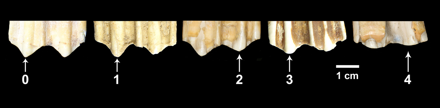
In this study, we used the extended mesowear methods proposed for equids (Kaiser and Solounias Reference Kaiser and Solounias2003) and ruminants (Franz-Odendaal and Kaiser Reference Franz-Odendaal and Kaiser2003). We collected mesowear data for teeth in middle stages of wear (i.e., heavily worn as well as very little worn teeth were not included in the analysis). Most of the specimens studied consisted of isolated teeth. In the case of horses, we recorded mesowear data from P4 to M3. For bison, we obtained mesowear data from M2 and M3; however, to increase sample size, in some cases we obtained mesowear data from M1 teeth. In some instances we encountered teeth belonging to the same individual. In those cases, we preferentially recorded mesowear data from the M2. If the M2 was damaged or absent, we randomly selected one of the other tooth positions that were well preserved. Sometimes we encountered specimens in which the right and left M2 were present in a good state of preservation. In those cases we selected one of the two teeth at random. We recorded mesowear data by direct observation of the specimens, and the frequency of the different variables was obtained for each sample. Subsequently, we calculated the mesowear score (Kaiser Reference Kaiser and Harrison2011), which combines cusp relief and shape into a single value: 0 (high and sharp cusps), 1 (high and round cusps), 2 (low and sharp cusps), 3 (low and round cusps), and 4 (low and blunt cusps) (Fig. 3). All of the teeth were examined and scored by the same researcher (C.I.B.-O.). Raw data are listed in Supplementary Table 2.

Figure 3. Buccal view of the molar cusps of five bison upper cheek teeth showing the mesowear score values considered in this study. 0 = high and sharp cusp; 1 = high and round cusp; 2 = low and sharp cusp; 3 = low and round cusp; 4 = low and blunt cusp.
We conducted Kruskal-Wallis tests (Hammer and Harper Reference Hammer and Harper2006) using the software PAST 2.17 (Hammer et al. Reference Hammer, Harper and Ryan2001) to assess whether the mesowear score significantly differed among sympatric bison and horse species. Significant differences would indicate dietary resource partitioning. The coevolutionary disequilibrium model predicts resource partitioning during preglacial/full-glacial time intervals, but not during the postglacial.
We also evaluated the variance of the mesowear score for each equid and bison sample and then calculated the quotient resulting from the division of the variance of the mesowear score at time interval 1 by the variance at time interval 2. Significance of the variance quotient was assessed by a two-sample F-test for equal variances (right-tailed) using the bootstrap resampling method (10,000 replicates) in MATLAB R2018a (MathWorks 2018; code available in Supplementary File 1). As predicted by the mosaic-nutrient extinction model, a reduction in variance of postglacial samples would reflect a reduction in the diversity of available vegetation for consumption by megaherbivores.
Analysis of Enamel Hypoplasia
Using both direct observations (n = 429) and observations on CT scans of specimens (n = 3), we analyzed a total of 432 specimens consisting mostly of isolated teeth (Supplementary Table 3) for both the presence/absence of enamel hypoplasia and the number of hypoplastic events present per affected tooth. We treated isolated teeth as separate individuals, unless there was evidence that isolated teeth were associated as part of the same tooth row, in which case the associated teeth were treated as a single individual. The sample included worn and unworn teeth to increase sample size. Any form of enamel hypoplasia was included in the analysis, because separation of the tooth defects into the categories established by the FDI for the study of enamel hypoplasia (FDI 1982) resulted in very small sample sizes. We calculated the percentage of specimens (i.e., individuals) presenting enamel hypoplasia in the different study samples to determine the prevalence of this tooth defect. We also calculated the mean number of hypoplastic events per affected tooth per sample, to shed light on the recurrence of episodes of systemic stress leading to hypoplasia during tooth development. To accomplish this task, we assumed that hypoplastic defects occurring at comparable heights on the same tooth crown resulted from the same stress event and could therefore be counted as a single hypoplastic event.
Initial assessments focused on a single tooth position; however, this resulted in very small sample sizes. We therefore included in the analysis as many complete teeth as we could reliably identify from various tooth positions. In the case of isolated teeth, we studied premolars (P2–P4; p2–p4) and molars (M1–M3; m1–m3) for equids, and molars for bison (M1–M3; m1–m3). We did not study premolars for bison, because the premolars are not molarized as they are in horses and as a result are morphologically different and much smaller than the molars. This difference in size could potentially bias the preservation of premolars in the fossil record relative to molars, and it could also affect their representation in research collections as a result of collecting biases. Moreover, the difference in size between premolars and molars of bison might indicate that these two tooth groups have a different dental developmental geometry, a factor that is known to affect the identification of enamel hypoplasia when using macroscopic methods (Hillson and Bond Reference Hillson and Bond1997; Hillson Reference Hillson2014).
When dealing with associated teeth (i.e., teeth belonging to the same individual), we examined either the P4 or M3 for enamel hypoplasia in addition to the M1 (p4 or m3, and m1 for lower teeth) in equids, and the M1, M2, and M3 (m1, m2, and m3 for lower teeth) in bison. This is because the timing of tooth crown formation in equids for the P4/p4 and M3/m3 minimally overlaps with the timing of crown formation for the M1/m1 (Hoppe et al. Reference Hoppe, Stover, Pascoe and Amundson2004). Thus, hypoplastic defects not occurring on the apical portion of the tooth crown (immediately below the area of the cusps) of the P4/p4 or M3/m3 can be identified as separate stress events from those present in the M1/m1. In bison the timing of tooth crown formation for each molar minimally overlaps (Gadbury et al. Reference Gadbury, Todd, Jahren and Amundson2000; Niven et al. Reference Niven, Egeland and Todd2004). Therefore, hypoplastic defects not occurring on the apical portion of the tooth crown (immediately below the area of the cusps), especially of M2/m2 and M3/m3, can be considered as distinct stress episodes. For a given individual, we noted the presence or absence of enamel hypoplasia on any of the teeth (Equus: P4 or M3, and M1 [p4 or m3, and m1 for lower teeth]; Bison: M1, M2, and M3 [m1, m2, and m3 for lower teeth]) and counted this as a single observation. This observation was added to the corresponding data set used to calculate the percentage of specimens presenting enamel hypoplasia for a specific study sample. We also added the number of hypoplastic events in each tooth considered (P4 or M3, and M1 in equids [p4 or m3, and m1 for lower teeth], and M1, M2, and M3 in bison [m1, m2, and m3 for lower teeth]) and divided this value by the number of teeth scored to determine the mean number of hypoplastic events per tooth. This result was included in the corresponding data set used to calculate the mean number of hypoplastic events per affected tooth for a specific study sample.
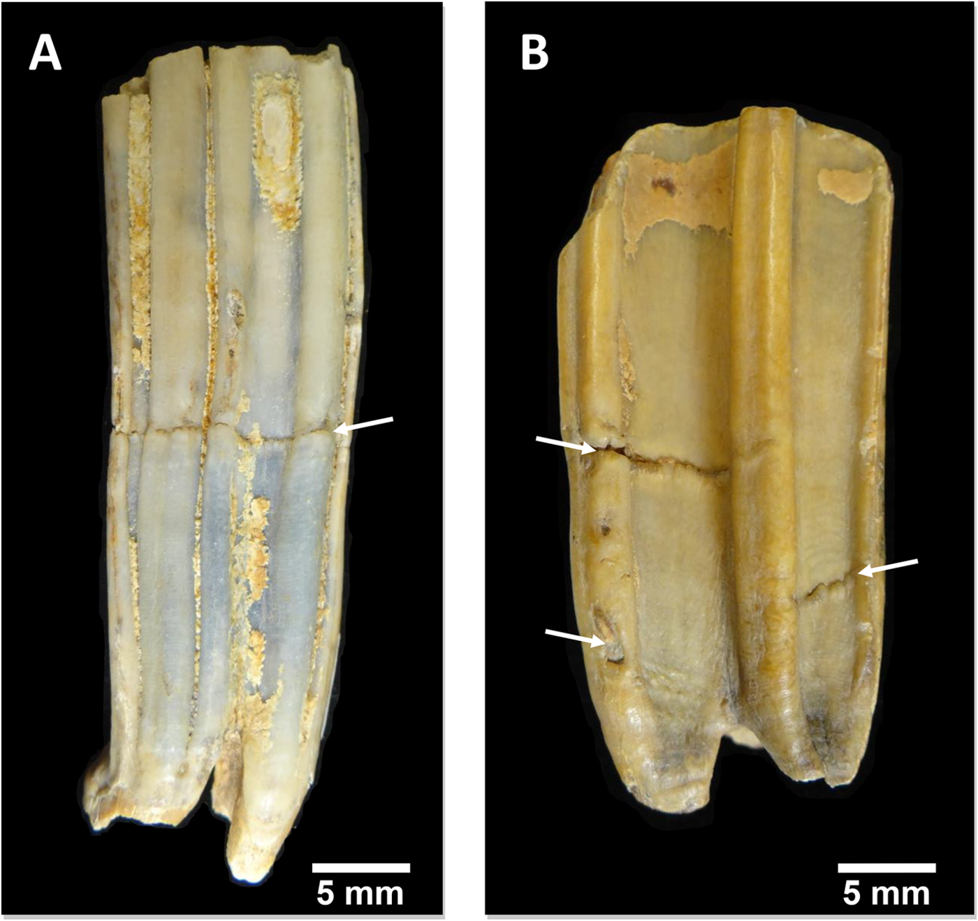
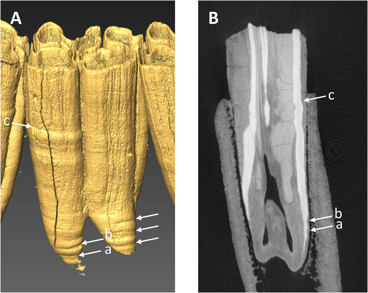
All of the specimens, except three equid dentaries from the Wally's Beach site, Alberta, were examined via direct observation (Fig. 4). We used oblique lighting to facilitate the identification of enamel hypoplasia. The vast majority of the equid cheek teeth from Wally's Beach are encased in dentaries or maxillaries, preventing the direct assessment of these specimens for enamel hypoplasia. Therefore, three dentaries from this site were CT-scanned to allow examination of the cheek teeth. The specimens were CT-scanned at the Department of Anthropology, University of Western Ontario, using a Nikon XT H 225 ST MicroCT Scanner with the following settings: 190 kVp, 85 microamps, 500 ms exposure time, averaged 2 frames/projection, and voxel size of 70 μm. The software Inspect-X v. 4.3 was used for scan capture, CT-Pro 3D v. 4.3 was used for volume reconstruction, and VG Studio Max v.2.2 was used for visualization and export to dicom. The CT-scan raw data we used are available in the Supplementary Material. We created 3D surface models of the CT-scanned specimens using the computer software AMIRA 5.3.3 for Mac OS X (Visage, Chelmsford, MA, http://www.visage.com). We adjusted the threshold to digitally remove the dentary and the cementum from the cheek teeth in order to be able to detect the presence of enamel hypoplasia on the surface of the tooth crown (Fig. 5A). We then prepared digital histological sections using the ObliqueSlice module in AMIRA 5.3.3 to verify that the tooth defects identified on the external surface of the tooth crown corresponded to enamel hypoplasia (Fig. 5B). All of the tooth defects identified in the 3D surface models showed thinning of the imbricational enamel (Fig. 5B), which is characteristic of enamel hypoplasia (Goodman and Rose Reference Goodman and Rose1990). These observations support the contention that similar tooth defects identified in the specimens that we assessed via direct observation corresponded to enamel hypoplasia. Only clearly defined, deep grooves were classified as enamel hypoplasia, following previous studies (e.g., Goodman and Rose Reference Goodman and Rose1990; Franz-Odendaal et al. Reference Franz-Odendaal, Chinsamy and Lee-Thorp2004).

Figure 4. Examples of equid cheek teeth illuminated with oblique lighting to highlight enamel hypoplasia (indicated by the white arrows). A, Lingual view of a lower left m1 (RAM P90.6.37). B, Buccal view of an upper right P4 (RAM P89.13.610).

Figure 5. Example of CT-scan data used to determine the presence of enamel hypoplasia in three equid mandibles from Wally's Beach, Alberta. A, Three-dimensional digital surface model of lower m1 (RAM DhPg-8 864) showing four hypoplastic events (horizontal linear grooves) indicated by the arrows. B, Radial digital section through the anterior portion of the same tooth showing the three hypoplastic events found on the protoconid column (a, b, c).
One potential complication of the study of enamel hypoplasia of equids and bison is the presence of cementum covering the tooth crown, which helps to anchor the tooth into the maxilla or dentary while the roots develop and the tooth erupts into the mouth (Kierdorf et al. Reference Kierdorf, Zeiler and Kierdorf2006; Upex et al. Reference Upex, Balasse, Tresset, Arbuckle and Dobney2014). Cementum did not pose a serious problem to the examination and study of enamel hypoplasia in our study, because weathering and degradation of cementum exposed the enamel underneath. When examining the specimens, we qualitatively scored the extent to which cementum covers the tooth crown using a scoring system that ranges from 0 to 5: 0 indicating that the tooth crown is not covered by cementum, 1 denoting that 1–25% of the tooth crown is covered by cementum, 2 indicating that 26–50% of the tooth crown is covered by cementum, 3 denoting that 51–75% of the tooth crown is covered by cementum, 4 indicating that 76–95% of the tooth crown is covered by cementum, but that the cementum present consists of a thin layer, and 5 denoting that the entire tooth crown is covered by a thick layer of cementum. We did not use specimens with a score of 5 in the analysis, because the cementum covering the tooth made it difficult to consistently evaluate whether enamel hypoplasia was present in the tooth. Some equid teeth from Bluefish Caves had one side of the tooth crown (the buccal side in lower teeth and the lingual side in upper teeth) completely covered by cementum, but not the remaining sides. We decided to score the exposed sides for enamel hypoplasia and include these specimens in the analysis, because otherwise the sample size for this locality would have been too low for statistical analysis.
For each geographic region and species, we conducted z-tests of proportions (left-tailed) to determine whether the percentage of specimens with enamel hypoplasia (i.e., prevalence of enamel hypoplasia) increased during the postglacial relative to the previous time interval(s). Similarly, we conducted t-tests (left-tailed) using the bootstrap resampling method (10,000 replicates) to determine whether the number of hypoplastic events per affected tooth increased during the postglacial, potentially indicating that stress events became more recurrent during this time interval as compared with full-glacial and preglacial intervals. We performed these tests for bison and equid samples separately, because it is not known whether both ungulate groups are equally sensitive to the development of enamel hypoplasia. Furthermore, the tooth crown of bison teeth develops faster than that of equids. For example, crown formation of the m3 takes on average 16 months in Plains bison (Niven et al. Reference Niven, Egeland and Todd2004), whereas it takes 34 months in domestic horse (Hoppe et al. Reference Hoppe, Stover, Pascoe and Amundson2004). Thus, equid teeth can potentially record more stress events than bison teeth, especially if these occurred periodically with a periodicity of up to 2.5 years in the longer-developing teeth such as the P4/p4, M2/m2, and M3/m3. All statistical tests were conducted using the software package MATLAB R2018a (MathWorks 2018) (code available in Supplementary Files 2 and 3). The significance level for all tests was set to a p-value of 0.05.
Assumptions and Limitations
Dental Wear
One of the primary assumptions made in this study is that consumption of different plant species and plant parts is recorded in the dental wear of herbivore teeth and that those differences can be observed at different scales (e.g., browser vs. grazer, or more importantly, differences within those broad categorizations). A large number of studies of dental wear at different scales and using different techniques (e.g., low-magnification microwear, texture microwear analysis, conventional mesowear, mesowear using the mesowear ruler) have consistently shown that dental wear varies significantly across broad dietary groups such as grazers, browsers, mixed feeders, frugivores, and generalists (e.g., Solounias et al. Reference Solounias, Teaford and Walker1988; Fortelius and Solounias Reference Fortelius and Solounias2000; Solounias and Semprebon Reference Solounias and Semprebon2002; Merceron et al. Reference Merceron, Blondel, de Bonis, Koufos and Viriot2005; Ungar et al. Reference Ungar, Merceron and Scott2007). However, finer dietary differences within these broad trophic groups have to be detected to test the extinction models considered here.
For example, the coevolutionary disequilibrium extinction model uses the present-day grazing succession of the African savannas as an example of a highly coevolved system (Graham and Lundelius Reference Graham, Lundelius, Martin and Klein1984). This particular system consists of several grazers, such as the plains zebra (Equus quagga), wildebeest (Connocaethes taurinus), hartebeest (Alcelaphus buselaphus), and topi (Damaliscus lunatus). Field studies have shown that in some areas, these grazers partition dietary resources by feeding on different plant parts and grasses at different growth stages (e.g., Gwynne and Bell Reference Gwynne and Bell1968; Bell Reference Bell1971; Murray and Brown Reference Murray and Brown1993). It is reasonable to propose that each of these grazers occupies a unique niche within the “grazer” spectrum and that there may be observable differences in tooth microwear and mesowear as a result. The results of a mesowear analysis of these ungulate mammals generally support this assumption (Fortelius and Solounias Reference Fortelius and Solounias2000).
The results of other dental wear studies (e.g., Scott Reference Scott2012; Barrón-Ortiz et al. Reference Barrón-Ortiz, Theodor and Arroyo-Cabrales2014) also indicate that it is possible to detect finer differences within the broad dietary groups that have traditionally been recognized. However, what those differences actually indicate about the feeding ecology of the ungulates investigated is less clear. Despite extensive research, there is still no consensus about the primary agent responsible for the formation of dental wear features. Phytoliths, lignin, and cellulose, as well as exogenous grit, have each been proposed as the primary factor producing dental wear (e.g., Walker et al. Reference Walker, Hoeck and Perez1978; Ungar et al. Reference Ungar, Teaford, Glander and Pastor1995; Merceron et al. Reference Merceron, Schulz, Kordos and Kaiser2007; Sanson et al. Reference Sanson, Kerr and Gross2007; Lucas et al. Reference Lucas, Omar, Al-Fadhalah, Almusallam, Henry, Michael and Arockia Thai2013; Schulz et al. Reference Schulz, Piotrowski, Clauss, Mau, Merceron and Kaiser2013; Tütken et al. Reference Tütken, Kaiser, Vennemann and Merceron2013). If phytoliths are the primary agent causing dental wear, then plants or plant parts differing in their concentration and type of phytoliths would produce different dental wear patterns. Alternatively, if exogenous grit is responsible for producing dental wear, then differences in dental wear may reflect feeding in different microhabitats (i.e., dusty vs. less dusty), or it may also reflect feeding on plant species or plant parts that differentially accumulate dust on their surface. More complexly, it is also possible that both exogenous grit and the physical properties of the vegetation contribute, or might even interact, to produce dental wear. While resolution of this issue is beyond the scope of this study, the assumption that differences that we observe are ecologically meaningful is essential and seems reasonable based on emerging data.
An additional assumption that we make in this study relates to the different digestive physiologies of equids and bison. Specifically, we assume that differences in digestive physiology of the investigated equid and bison species do not significantly bias dental wear patterns. Equids are hindgut fermenters with high chewing efficiency and rapid passage times. They consume large amounts of plant material, and that material passes rapidly through the digestive system and is then fermented by microbial activity in the caecum (Janis Reference Janis1976; Clauss et al. Reference Clauss, Nunn, Fritz and Hummel2009). Equids also have molarized premolars that greatly assist in the mechanical breakdown of plant material (Janis Reference Janis, Russell, Santoro and Sigogneau-Russell1988), possess highly hypsodont teeth (Janis Reference Janis, Russell, Santoro and Sigogneau-Russell1988), and have a greater enamel complexity than bison (Famoso et al. Reference Famoso, Feranec and Davis2013).
Bison are ruminant foregut fermenters and have a four-chambered stomach in which microbial fermentation of plant material occurs in the rumen, the first chamber of the stomach (Janis Reference Janis1976). To complement the fermentation process, ruminants periodically regurgitate the food located in the rumen and rechew it (Janis Reference Janis1976). The second (reticulum) and third (omasum) chambers act as filters, and the fourth chamber (abomasum) is the true stomach (Janis Reference Janis1976). The digestive system of ruminants achieves a high degree of particle size reduction, greater than that observed for hindgut fermenters and nonruminant foregut fermenters (Fritz et al. Reference Fritz, Hummel, Kienzle, Arnold, Nunn and Clauss2009).
Few studies have investigated whether differences in digestive physiology systematically bias the dental wear patterns produced. A recent study that examined microwear on occlusal enamel bands located in the lingual, center, and buccal sides of upper molars of eight species of ruminants and perissodactyls found that microwear features were distributed homogeneously across ruminant molars, but not in the perissodactyl molars (Mihlbachler et al. Reference Mihlbachler, Campbell, Ayoub, Chen and Ghani2016). In the latter group, microwear features from the labial side of the molars were more strongly predictive of diet (Mihlbachler et al. Reference Mihlbachler, Campbell, Ayoub, Chen and Ghani2016); however, further studies examining more specimens and additional taxa are needed to corroborate these patterns.
Enamel Hypolasia
Testing of the coevolutionary disequilibrium (Graham and Lundelius Reference Graham, Lundelius, Martin and Klein1984) and mosaic-nutrient (Guthrie Reference Guthrie, Martin and Klein1984) extinction models requires assessment of nutritional stress in Pleistocene herbivore mammals. Several studies indicate that enamel hypoplasia can be associated with nutritional stress (e.g., Goodman and Rose Reference Goodman and Rose1990; Hillson Reference Hillson1996; Larsen Reference Larsen1997; Zhou and Corruccini Reference Zhou and Corruccini1998; Dobney and Ervynck Reference Dobney and Ervynck2000; Hillson Reference Hillson2005; Guatelli-Steinberg and Benderlioglu Reference Guatelli-Steinberg and Benderlioglu2006), and we make the assumption that our observations of hypoplasia are reflective of that stress. That said, we acknowledge that this tooth defect has a multifactorial etiology, and a variety of other stressors, in addition to malnutrition, have been associated with its development. Systemic and infectious diseases, severe fevers, premature births, parturition, weaning, parasite infestation, and intoxication with fluoride are some of the stressors linked to the development of enamel hypoplasia in mammals (Shearer et al. Reference Shearer, Kolstad and Suttie1978; Shupe and Olson Reference Shupe, Olson, Shupe, Peterson and Leone1983; Skinner and Hung Reference Skinner and Hung1986; Suckling et al. Reference Suckling, Elliott and Thurley1986, Reference Suckling, Thurley and Nelson1988; Miles and Grigson Reference Miles and Grigson1990; Kierdorf et al. Reference Kierdorf, Kierdorf and Fejerskov1993, Reference Kierdorf, Kierdorf, Richards and Sedlacek2000, Reference Kierdorf, Kierdorf, Richards and Josephsen2004; Hillson Reference Hillson1996, Reference Hillson2005; Larsen Reference Larsen1997; Dobney and Ervynck Reference Dobney and Ervynck2000). Inferring which stressor potentially caused enamel hypoplasia in a given individual cannot be accomplished without additional lines of evidence, such as knowledge of the diet and life history of the species under study (e.g., Dobney and Ervynck Reference Dobney and Ervynck2000; Franz-Odendaal et al. Reference Franz-Odendaal, Chinsamy and Lee-Thorp2004; Niven et al. Reference Niven, Egeland and Todd2004). Therefore, the presence of enamel hypoplasia is more commonly treated as an indicator of overall health during tooth development. In that sense, any indication of hypoplasia would be consistent with nutritional stress, but not necessarily indicative of nutritional stress.
Results
Microwear
The summary statistics of the microwear variables of the late Pleistocene equid and bison samples studied are shown in Table 2. The analysis of the low-magnification microwear data (Supplementary Table 1) indicates statistically significant differences in some of the samples studied for evaluating the hypotheses of the coevolutionary disequilibrium extinction model. The NP-MANOVA test (Table 3) reveals that the microwear pattern of “E. conversidens” from the American Southwest is marginally statistically different from the microwear pattern of E. “ferus” for the full-glacial time interval (F = 1.713, p = 0.0496). In contrast, the microwear pattern of these two equid species, as well as that of B. antiquus, is not significantly different for the postglacial (NP-MANOVA test, F = 0.8747, p = 0.6263). In the case of the specimens from Alberta, the comparison of the horse and bison samples for the preglacial time interval is marginally not significant (NP-MANOVA test, F = 1.556, p = 0.0790), likely due to the small sample sizes for these species. The microwear patterns of postglacial horse and bison samples from Alberta are not statistically different (NP-MANOVA test, F = 0.9605, p = 0.5284).
Table 2. Summary statistics of microwear variables of late Pleistocene equid and bison samples studied. n = number of specimens; s = average number of scratches; p = average number of pits; cs = average number of cross scratches; lp = average number of large pits; g = average gouge score, ranging from 0 (none present) to 1 (all enamel bands observed had at least 1 gouge present); ws = average number of wide scratches; ts = average texture score.

Table 3. Results of NP-MANOVA tests (10,000 replications and using the Mahalanobis distance measure) used to evaluate the hypotheses of the coevolutionary disequilibrium extinction model using the variables in Supplementary Table 1. n = sample size; F = F-statistic; p = p-value. Statistically significant p-values are shown in bold.

The variance of the five counted microwear variables of each species sample did not significantly decrease during the postglacial relative to full-glacial and preglacial time intervals (Table 4). Only two pairwise comparisons are statistically significant, and four other comparisons show the opposite trend, in which the variance significantly increased during the postglacial (Table 4).
Table 4. Results of two-sample F-tests for equal variances (right-tailed) using the bootstrap resampling method (10,000 replicates) conducted to test the hypotheses of the mosaic-nutrient extinction model using four counted microwear variables: s = average number of scratches; p = average number of pits; cs = average number of cross scratches; lp = average number of large pits; ws = average number of wide scratches; VarQ = variance quotient (variance at time interval 1 divided by variance at time interval 2); p = p-value. Statistically significant p-values are indicated in bold. An asterisk (*) identifies comparisons in which the variance at time interval 2 is greater than at time interval 1.

Mesowear
Overall, the mean mesowear score of each sample analyzed (Table 5) plots on the abrasion end of the mesowear spectrum (Fig. 6). The mesowear score of “E. conversidens” from the American Southwest is not statistically different from the mesowear score of E. “ferus” for the full-glacial time interval (Kruskal-Wallis test, H = 1.00, p = 0.2834), although it should be pointed out that the sample size of “E. conversidens” consists of only two specimens (Table 6). The mesowear scores for these two equid species, along with the specimens of B. antiquus, for the postglacial of the American Southwest are also not significantly different (Kruskal-Wallis test, H = 1.309, p = 0.4851). The Kruskal-Wallis test reveals that the mesowear score for the preglacial samples of horse and bison from Alberta are significantly different (H = 5.442, p = 0.0134), but this is not the case for the postglacial samples of these ungulates (H = 1.771, p = 0.1582).

Figure 6. Average mesowear score for the late Pleistocene bison and equid samples studied and extant ungulate species reported in Kaiser et al. (Reference Kaiser, Müller, Fortelius, Schulz, Codron and Claus2013). Each data point is the average for a species sample. Abbreviations: LB = leaf browsers; MF = mixed feeders; G = grazers; Pre-LGM = preglacial; LGM = full-glacial; Post-LGM = postglacial; BaS = Bison antiquus (American Southwest); BpA = Bison sp. (Alberta); EcS = “Equus conversidens” (American Southwest); EfA = Equus “ferus” (Alberta); EfB = E. “ferus” (Bluefish Caves, Yukon); EfS = E. “ferus” (American Southwest).
Table 5. Summary statistics of the mesowear variables of late Pleistocene equid and bison samples studied. n = number of specimens; MS = mesowear score; h = percentage of specimens with high occlusal relief; l = percentage of specimens with low occlusal relief; s = percentage of specimens with sharp cusps; r = percentage of specimens with round cusps; b = percentage of specimens with blunt cusps.

Table 6. Results of Kruskal-Wallis tests used to evaluate the hypotheses of the coevolutionary disequilibrium extinction model using the mesowear score (MS). n = sample size; H = H-statistic; p = p-value. Statistically significant p-values are shown in bold.
The variance of the mesowear score of each species sample did not significantly decrease during the postglacial relative to full-glacial and preglacial time intervals (Table 7). None of the pairwise comparisons are statistically significant, and in one comparison (preglacial vs. postglacial samples of “E. conversidens” from the American Southwest), the opposite trend was observed (Table 7).
Table 7. Results of two-sample F-tests for equal variances (right-tailed) using the bootstrap resampling method (10,000 replicates) conducted to test the hypotheses of the mosaic-nutrient extinction model using the mesowear score (MS). Var = variance of each sample; VarQ = variance quotient (variance at time interval 1 divided by variance at time interval 2); p = p-value. Statistically significant p-values are indicated in bold. An asterisk (*) identifies comparisons in which the variance at time interval 2 is greater than at time interval 1.

Enamel Hypoplasia
Enamel hypoplasia was observed in all equid and bison samples studied. The prevalence of this tooth defect showed a larger range in equids than in bison. The prevalence of enamel hypoplasia in the equid samples ranged from 31.25% in the preglacial sample of “E. conversidens” from the American Southwest to 64.29% in the postglacial sample of E. “ferus” from Alberta (Fig. 7; Table 8). In contrast, the prevalence of enamel hypoplasia in the bison samples ranged from 25.71% in the preglacial sample of Bison sp. from Alberta to 29.41% in the postglacial samples of Bison sp. from Alberta and B. antiquus from the American Southwest (Fig. 7; Table 8).
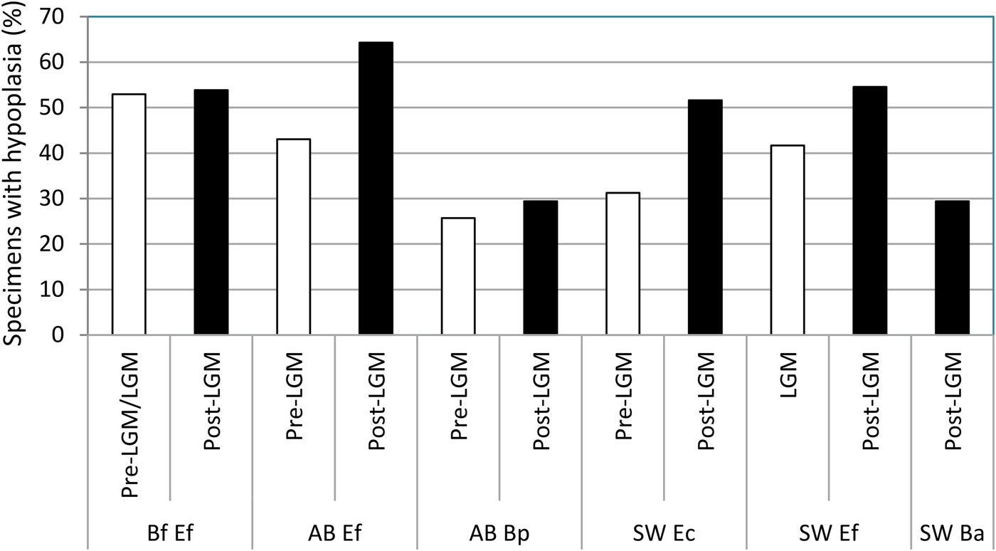
Figure 7. Prevalence of enamel hypoplasia in the equid and bison samples studied. Bf Ef = Equus “ferus,” Bluefish Caves; AB Ef = E. “ferus,” Alberta; AB Bp = Bison sp., Alberta; SW Ec = “Equus conversidens,” American Southwest; SW Ef = E. “ferus,” American Southwest; SW Ba = Bison antiquus, American Southwest. Time interval abbreviations: Pre-LGM = preglacial; LGM = full-glacial; Post-LGM = postglacial.
Table 8. Summary statistics of enamel hypoplasia data for the equid and bison samples studied. n = total number of specimens examined; H = number of specimens with enamel hypoplasia; PH = percentage of specimens with enamel hypoplasia; ME = mean number of hypoplastic events per affected specimen.

The prevalence of enamel hypoplasia in equids increased during the postglacial in two out of four samples in which this comparison was made (Table 9). The sample of “E. conversidens” from the American Southwest shows a prevalence of enamel hypoplasia of 31.25% for the preglacial and 51.61% for the postglacial, and this difference is statistically significant (z-test of proportions, z = −1.8099, p = 0.0352). Similarly, the frequency of enamel hypoplasia of E. “ferus” from Alberta increased from 43.05% in the preglacial to 64.29% during the postglacial. This is the largest increase in enamel hypoplasia of the samples we studied, although this difference only approaches statistical significance (z-test of proportions, z = −1.5286, p = 0.0632) because of the reduced sample size of the postglacial sample. We predict that this trend will be further supported with the discovery and analysis of more specimens of appropriate geologic age. The prevalence of enamel hypoplasia for the postglacial sample of E. “ferus” from Bluefish Caves is not significantly greater than the prevalence calculated for the preglacial/full-glacial interval (53.85% vs. 52.94%; z = −0.0492, p = 0.4804). Also not significant is the comparison of the full-glacial (41.67%) and postglacial (54.55%) samples of E. “ferus” from the American Southwest (z-test of proportions, z = −0.8092, p = 0.2092), as well as preglacial (25.71%) and postglacial (29.41%) Bison sp. samples from Alberta (z-test of proportions, z = −0.3437, p = 0.3655).
Table 9. Results of z-tests of proportions (left-tailed) used to determine whether the incidence of enamel hypoplasia significantly increased during the postglacial relative to the previous time interval(s). n = total number of specimens examined; PH = percentage of specimens with enamel hypoplasia; z = z-statistic; p = p-value. Statistically significant p-values are shown in bold. “Equus conversidens” from the American Southwest for the full-glacial interval was excluded from the analysis because of its small sample size.

The average number of hypoplastic events per affected tooth increased during the postglacial in all of the equid pairwise comparisons except one (Fig. 8; Table 10). The largest increase was observed in E. “ferus” from Bluefish Caves, in which the average number of hypoplastic events per affected tooth increased from 1.33 in the preglacial/full-glacial interval to 3.43 in the postglacial (t-test, t = −4.062, p = 0.0000). The average number of hypoplastic events also increased in the equid samples from the American Southwest, where it went from 1.23 in the preglacial to 1.78 in the postglacial for “E. conversidens” (t-test, t = −1.963, p = 0.0297) and 1.60 in the full-glacial to 2.30 in the postglacial for E. “ferus” (t-test, t = −2.246, p = 0.0437). Contrary to these trends, the average number of hypoplastic events per affected tooth significantly decreased during the postglacial in E. “ferus” from Alberta (2.16 events in the preglacial versus 1.37 in the postglacial; t-test [right-tailed], t = 2.338, p = 0.0128), whereas in Bison sp. from the same geographic region, the average number of events appears to remain constant in the preglacial (1.31) as in the postglacial (1.30) (t-test, t = 0.029, p = 0.5287).
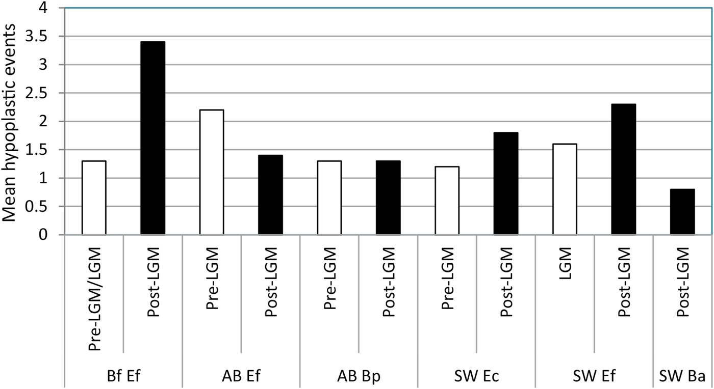
Figure 8. Mean number of hypoplastic events per affected specimen in the equid and bison samples studied. Bf Ef = Equus “ferus,” Bluefish Caves; AB Ef = E. “ferus,” Alberta; AB Bp = Bison sp., Alberta; SW Ec = “Equus conversidens,” American Southwest; SW Ef = E. “ferus,” American Southwest; SW Ba = Bison antiquus, American Southwest. Time interval abbreviations: Pre-LGM = preglacial; LGM = full-glacial; Post-LGM = postglacial.
Table 10. Results of t-tests (left-tailed) using the bootstrap resampling method (10,000 replicates) to determine whether the number of stress events per affected specimen increased during the postglacial relative to the previous time interval(s). nH = total number of specimens with enamel hypoplasia; ME = mean number of hypoplastic events per affected specimen; t = t-statistic; p = p-value. Statistically significant p-values are shown in bold. An asterisk (*) identifies comparisons in which the mean number of hypoplastic events per affected specimen significantly decreased during the postglacial (i.e., showing a trend opposite to the one being tested). “Equus conversidens” from the American Southwest for the full-glacial interval was excluded from the analysis because of its small sample size.
Discussion
Dental Wear Patterns and Nutritional Extinction Models
The coevolutionary disequilibrium (Graham and Lundelius Reference Graham, Lundelius, Martin and Klein1984) and mosaic-nutrient (Guthrie Reference Guthrie, Martin and Klein1984) extinction models are two climate-based models that were proposed to explain the late Pleistocene megafaunal extinction. The coevolutionary disequilibrium model emphasizes competition for food resources among species as a result of changing vegetational assemblages (Graham and Lundelius Reference Graham, Lundelius, Martin and Klein1984), whereas the mosaic-nutrient model proposes that a change from a mosaic vegetation pattern to a more zonal, low-diversity pattern decreased the dietary supplements available to herbivores (Guthrie Reference Guthrie, Martin and Klein1984). Although these models present different scenarios that lead to nutritional stress and extinction of some herbivore species, they are not mutually exclusive. In theory both could have operated, resulting in a scenario in which herbivores were faced with a decreased diversity of plants in their diets and a disruption of coevolved foraging sequences, increasing competition among species. However, the results of our analyses are overall consistent with the predictions established for the coevolutionary disequilibrium model, but not with the prediction established for the mosaic-nutrient model.
The results of the analysis of dental wear are overall consistent with the two predictions established for the coevolutionary disequilibrium extinction model. The first prediction states that before the severe climatic changes that occurred during the terminal Pleistocene, sympatric species of ungulate herbivores partitioned available food resources (Graham and Lundelius Reference Graham, Lundelius, Martin and Klein1984). In this case dietary niche partitioning would be reflected by a statistically significant difference in dental microwear and mesowear score. This prediction is generally supported for the ungulates studied from the American Southwest and Alberta (Tables 3 and 6). The dental microwear of “E. conversidens” and E. “ferus” from the American Southwest during the full-glacial is significantly different (Table 3), and statistically significant differences were also detected for the mesowear score of E. “ferus” and Bison sp. from preglacial deposits of Alberta (Table 6).
Although the results of the microwear and mesowear analyses support the hypothesis of dietary resource partitioning in sympatric bison and equid species from the American Southwest and Alberta before the postglacial, the analysis of dental wear provides little insight into the mechanism by which this division of resources might have taken place. Extant ungulates partition dietary resources in a variety of ways: feeding on different plant species, feeding on different plant parts and growth stages of the same species, feeding at different heights, and feeding in distinct microhabitats (e.g., Bell Reference Bell1971; Jarman and Sinclair Reference Jarman, Sinclair, Sinclair and Norton-Griffiths1979; McNaughton and Georgiadis Reference McNaughton and Georgiadis1986; du Toit Reference Du Toit1990; Spencer Reference Spencer1995; Stewart et al. Reference Stewart, Bowyer, Kie, Cimon and Johnson2002). Dental wear data alone cannot determine which of these alternatives for partitioning food resources was employed by the bison and equid species studied. Additional lines of evidence, such as stable isotope analysis and ecomorphological studies, in conjunction with the results of dental wear are needed to establish hypotheses as to how these ungulates might have partitioned dietary resources.
The second prediction outlined for the coevolutionary disequilibrium extinction model states that sympatric species of horse and bison were competing for available food resources during the terminal Pleistocene as a result of change in the composition of vegetational communities. Under this scenario dental microwear and mesowear should not be significantly different for bison and horse at the end of the Pleistocene. This is the pattern that is observed for the postglacial ungulate species from the American Southwest (i.e., “E. conversidens,” E. “ferus,” and B. antiquus; Tables 3 and 6). The same was found for the horse and bison samples of E. “ferus” and Bison sp. from postglacial deposits of Alberta (Tables 3 and 6). The results of the microwear and mesowear analyses of the postglacial ungulate species from the American Southwest and Alberta are, therefore, consistent with the second prediction of the coevolutionary disequilibrium extinction model.
The results of a number of dental wear (Rivals et al. Reference Rivals, Schulz and Kaiser2008, Reference Rivals, Mihlbachler, Solounias, Mol, Semprebon, de Vos and Kalthoff2010) and stable isotope (Koch et al. Reference Koch, Hoppe and Webb1998; Hoppe and Koch Reference Hoppe, Koch and Webb2006; Sánchez et al. Reference Sánchez, Prado and Alberdi2006; Fox-Dobbs et al. Reference Fox-Dobbs, Leonard and Koch2008) studies also support the assumption of dietary resource partitioning postulated for the coevolutionary disequilibrium extinction model. In other cases, however, dietary niche overlap is the emerging pattern (e.g., Feranec Reference Feranec2004; Prado et al. Reference Prado, Alberdi, Azanza, Sanchez and Frassinetti2005; Hoppe and Koch Reference Hoppe, Koch and Webb2006; Fox-Dobbs et al. Reference Fox-Dobbs, Leonard and Koch2008; Pérez-Crespo et al. Reference Pérez-Crespo, Arroyo-Cabrales, Alva-Valdivia, Morales-Puente and Cienfuegos-Alvarado2012). Nevertheless, it is important to point out that all of the studies cited, and also the study presented here, examined only one or two dietary proxies, which shed light on only a small portion of the feeding ecology of the Pleistocene megafauna.
Dietary niche partitioning may occur along any of countless multidimensional axes (Hutchinson Reference Hutchinson1957). Therefore, identification of statistically significant differences among species using one dietary proxy would provide support for dietary niche partitioning, but the opposite is not true. Inability to detect significant differences among species using one dietary proxy does not necessarily indicate they were competing for food resources, because the species could be segregating along another dimensional axis not considered in the study. This is an important point that is often missed in paleoecological studies. A multiproxy approach to reconstructing feeding ecology is required to better elucidate community feeding structure during the Pleistocene at different temporal and spatial scales. In that sense, the results of our study may be reevaluated as additional paleoecological proxies (e.g., stable isotope analysis) become available. With that consideration, we conclude that the analyses of mesowear and dental microwear do not reject the hypothesis of competition for food resources during the postglacial in the bison and equid samples investigated.
We note that a pattern consistent with competition for resources was recovered for bison and horse in both Alberta and the American Southwest, even though these two regions experienced different ecosystem dynamics during the terminal Pleistocene. Preglacial ecosystems in Alberta were completely eliminated during the full-glacial by the advance and coalescence of the Laurentide and Cordilleran ice sheets (Young et al. Reference Young, Burns, Smith, Arnold and Rains1994, Reference Young, Burns, Rains and Schowalter1999; Burns Reference Burns1996). Radiocarbon dating of mammalian specimens indicates that most of Alberta remained covered by the ice sheets for approximately 9000 radiocarbon years (Burns Reference Burns1996). As the ice sheets receded, new ecosystems with new community associations were established. In contrast to Alberta, the American Southwest was not covered by ice sheets; nevertheless, important environmental changes occurred in this region during the postglacial. Paleontological and palynological evidence indicates that the American Southwest experienced significant changes in temperature, precipitation, and humidity (Connin et al. Reference Connin, Betancourt and Quade1998; Polyak et al. Reference Polyak, Asmerom, Burns and Lachniet2012). Both regions experienced different, but nonetheless major, ecological disturbances during the terminal Pleistocene.
In contrast to the support for the coevolutionary disequilibrium model, our analyses of microwear and mesowear were less consistent with the mosaic-nutrient extinction model. Working under the assumption that feeding on different vegetation is reflected in the dental wear pattern, a population of herbivores feeding on a restricted number of plant species during the terminal Pleistocene would produce a dental wear sample in which the statistical dispersion of the microwear and mesowear variables is small relative to populations feeding on a greater diversity of plant species during preglacial and full-glacial times. Analyses of the dental wear data do not support this prediction (Tables 4 and 7). The variance of the microwear variables and the mesowear score are, for the most part, not significantly smaller during the postglacial. Only two pairwise comparisons involving the postglacial were statistically significant, and five other comparisons showed the opposite trend, with a significantly greater variance during the postglacial (Tables 4 and 7). There are a number of potential explanations that can be advanced to account for the lack of a statistically significant decrease in dental wear variance during the postglacial: 1) local plant diversity did not actually decrease during the postglacial; 2) local plant diversity decreased, but ungulates were able to extend their home ranges or migrate to obtain the right mix of nutrients; or 3) local plant diversity decreased, but the resulting change in diet is not recorded in the dental wear. The consistency of our results with these potential explanations are beyond the scope of this study, but we do stress that the evaluation of our results in the context of regional paleoenvironmental studies may be possible with comparisons to pollen records (e.g., Ritchie et al. Reference Ritchie, Cinq-Mars and Cwynar1982; Anderson et al. Reference Anderson, Edwards, Brubaker, Gillespie, Porter and Atwater2003; Hall Reference Hall, Lucas, Morgan and Zeigler2005; Strong and Hills Reference Strong and Hills2005; Zazula et al. Reference Zazula, Schweger, Beaudoin and McCourt2006), plant macrofossil records (e.g., Lamb and Edwards Reference Lamb, Edwards, Huntley and Webb1988; Hall Reference Hall, Lucas, Morgan and Zeigler2005; Zazula et al. Reference Zazula, Schweger, Beaudoin and McCourt2006), and studies on ancient DNA from soils (e.g., Willerslev et al. Reference Willerslev, Davison, Moora, Zobel, Coissac, Edwards and Lorenzen2014).
Implications for a New Ecological Extinction Model
One emerging pattern common to Alberta, the American Southwest, and other regions of North America is the increased abundance of bison relative to other large herbivorous mammals, including equids and mammoth, during the latest Pleistocene. Although both bison and equids returned to Alberta as the Laurentide and Cordilleran ice sheets receded, bison became the most abundant ungulate species, in contrast to preglacial ecosystems in which equids had higher abundances relative to bison (Jass et al. Reference Jass, Burns and Milot2011). A similar increase in the relative abundance of bison was reported for the midcontinent of North America (McDonald Reference McDonald1981), Alaska and the Yukon Territory (Guthrie Reference Guthrie2006), the southern Great Plains (Wyckoff and Dalquest Reference Wyckoff and Dalquest1997), and the Pacific Coast (Scott Reference Scott2010). The great abundance and geographic distribution of bison during the latest Pleistocene, especially in western North America, led to a recently proposed ecological extinction model for the late Pleistocene megafaunal extinctions in which bison played a pivotal role (Scott Reference Scott2010).
One major difference of the Pleistocene–Holocene transition with respect to previous glacial–interglacial transitions was the proliferation of bison, especially B. antiquus, a large, herd-dwelling ruminant (Scott Reference Scott2010). The ecological extinction model recently advanced proposes that bison and other late Pleistocene megafauna, including mammoths and equids, were competing for available resources (Scott Reference Scott2010). Shifts in resource abundance and distribution due to changing climatic factors associated with the end of the Wisconsinan glaciation would have increased competition for those resources, and typical responses of large herbivorous mammals to earlier climatic shifts (e.g., selection of different forage, reduction of body size, or migration to a different area) would have been altered by the widespread abundance and population density of bison. Even communities where bison were rare or absent could also be impacted, as large mammals displaced by bison in other regions moved in, increasing the competition among herbivores (Scott Reference Scott2010).
Isotope data for herbivorous mammals from Rancho La Brea, California, and Florida have been cited to support the argument that bison competed for resources with other late Pleistocene megafauna. Bison and equids from Rancho La Brea seemed to have relied heavily on C3 plants (Coltrain et al. Reference Coltrain, Harris, Cerling, Ehleringer, Dearing, Ward and Allen2004; Feranec et al. Reference Feranec, Hadly and Paytan2009), with bison periodically incorporating C4 plants in their diet, suggesting that these ungulates were seasonally competing for food resources (Feranec et al. Reference Feranec, Hadly and Paytan2009). Similar results have been reported for Florida, where mammoths, bison, and equids apparently had similar diets, although these diets varied geographically across the state (Feranec Reference Feranec2004). However, the fact that these herbivorous mammals fed on plants with similar isotope compositions does not necessarily imply that they were competing for food resources. For instance, African grazing ungulates feed mostly on C4 grasses, and their mean δ13C values largely overlap (e.g., Cerling et al. Reference Cerling, Harris and Passey2003), yet many of these grazing herbivores partition available grass resources by feeding on different structural components and/or grasses at different growth stages (e.g., Gwynne and Bell Reference Gwynne and Bell1968; Bell Reference Bell1971; Murray and Brown Reference Murray and Brown1993). As emphasized by McNaughton and Georgiadis (Reference McNaughton and Georgiadis1986), grass is not a homogeneous resource, and nutritional quality varies among its major structural components (leaf, sheath, and stem) as well as seasonally.
Based on the results obtained from the present study, the pattern of competition among bison and other late Pleistocene ungulates postulated by Scott (Reference Scott2010) is supported for the equid and bison samples from the postglacial of Alberta and the American Southwest, but not for the preglacial of Alberta. Overall, the pattern in our data is more consistent with the coevolutionary disequilibrium extinction model (Graham and Lundelius Reference Graham, Lundelius, Martin and Klein1984) than with the model proposed by Scott (Reference Scott2010). However, additional studies are needed to further validate the patterns presented in our study and evaluate these two extinction models.
Systemic Stress in Late Pleistocene Equids and Bison
Both the coevolutionary disequilibrium (Graham and Lundelius Reference Graham, Lundelius, Martin and Klein1984) and mosaic-nutrient (Guthrie Reference Guthrie, Martin and Klein1984) extinction models propose that populations of large mammals, especially the species that became extinct, were exposed to increased levels of systemic physiological stress, particularly nutritional stress, resulting from climatic and environmental changes. The results of the analysis of enamel hypoplasia of late Pleistocene equids and bison from the Western Interior of North America indicate that disruptions in tooth development, particularly in the equid taxa studied, increased during the postglacial relative to earlier time intervals. Working under the assumption that enamel hypoplasia primarily reflects episodes of systemic stress (Goodman and Rose Reference Goodman and Rose1990), these results support the hypothesis that equids experienced increased levels of systemic physiological stress during the postglacial. In all of the equid samples studied, the prevalence of enamel hypoplasia and/or recurrence of hypoplastic events increased during this time interval (Tables 9 and 10). However, we note that these changes were not spatially or temporally uniform.
The specimens of E. “ferus” from Bluefish Caves show that although the prevalence of enamel hypoplasia did not significantly change from the preglacial/full-glacial to the postglacial (both time intervals show a prevalence of hypoplasia of ~53%), the number of hypoplastic events per affected tooth significantly increased during the postglacial from 1.33 to 3.43. These results indicate that E. “ferus” in eastern Beringia, which apparently was already exposed to relatively high levels of systemic stress during the preglacial/full-glacial, with more than 50% of the specimens showing enamel hypoplasia, experienced more recurrent severe stress events during the postglacial. Assuming that the average cheek tooth of extinct populations of E. “ferus” took approximately 26 months to form, as is the case for extant domestic horses (Hoppe et al. Reference Hoppe, Stover, Pascoe and Amundson2004), some of the postglacial specimens of E. “ferus” were experiencing more than one severe stress event in a single year.
In Alberta, postglacial specimens of E. “ferus” show a greater prevalence of enamel hypoplasia, with 64.29% of specimens displaying a hypoplastic defect as compared with the preglacial sample, in which the prevalence is 43.05%. Contrary to the increase in the prevalence of hypoplasia, the number of hypoplastic events per affected tooth is significantly smaller in the postglacial (1.37) than in the preglacial (2.16). These results might indicate that stress events encountered by E. “ferus” from Alberta were less recurrent during the postglacial, but when they did occur, they were more severe, affecting a greater proportion of individuals. In contrast to these results, the postglacial sample of Bison sp. from Alberta does not show a significantly greater prevalence of enamel hypoplasia or a greater number of hypoplastic events per affected tooth than preglacial specimens. This suggests that, in contrast to E. “ferus,” Bison sp. did not endure significantly greater levels of systemic stress during the postglacial relative to what members of this ungulate group encountered during preglacial times.
The two equid species studied from the American Southwest, “E. conversidens” and E. “ferus,” show an increase in the average number of hypoplastic events per affected tooth during the postglacial. In the case of “E. conversidens” the number of hypoplastic events significantly increased from 1.23 in the preglacial to 1.78 in the postglacial, whereas in E. “ferus” it increased from 1.60 in the full-glacial to 2.30 in the postglacial. The prevalence of enamel hypoplasia also increased during the postglacial in both equid species, but it was only statistically significant in “E. conversidens,” which shows an increase from 31.25% in the preglacial to 51.61% in the postglacial. These results suggest that episodes causing systemic stress might have increased in severity and also probably became more recurrent. The postglacial sample of B. antiquus shows comparable levels of hypoplasia as the preglacial and postglacial Bison sp. samples from Alberta, with a hypoplasia prevalence of 29.41%.
The implication of the results of our evaluation of hypoplasia for the late Pleistocene extinction debate requires a determination of whether the prevalence and number of hypoplastic defects, especially for postglacial equid samples, are sufficiently high to suggest a dramatic increase in the morbidity of these ungulates. Unfortunately, data on enamel hypoplasia and its relationship to population dynamics in extant wild equids are lacking, but for bison there are some data on the prevalence of enamel hypoplasia in extant wild populations.
Bison examined as part of a macroscopic study of dental pathologies in terminal Pleistocene and Holocene archaeological assemblages included a collection of modern bison specimens from Montana (collected in 1886) and Yellowstone (donated to the Smithsonian Institution between 1909 and 1919; Byerly Reference Byerly2009). The prevalence of enamel hypoplasia in the individuals with the cemento-enamel junction visible is 22.2% for the sample from Montana and 25.0% for Yellowstone, although the sample size for the latter is very small, with only 4 individuals versus 27 for the sample from Montana (Byerly Reference Byerly2009). These values are relatively lower than those obtained for the postglacial bison samples from Alberta and the American Southwest.
The prevalence of enamel hypoplasia in the archaeological assemblages studied by Byerly (Reference Byerly2009), for samples greater than 10, ranges from 7.7% in the Horner I assemblage, Wyoming (~9500 yr RCBP [radiocarbon years before the present]), to 36.8% in the Frasca site, Colorado (~8900 yr RCBP). Comparable values were reported for Buffalo Creek, Wyoming (~2500 yr RCBP), and Kaplan-Hoover, Colorado (~2700 yr RCBP), in which 32.3% and 14.1%, respectively, of the molars examined show enamel hypoplasia (Niven et al. Reference Niven, Egeland and Todd2004). In this context, the prevalence of hypoplasia in postglacial bison samples from Alberta and the American Southwest is within the upper range reported for Holocene samples. At the least, this shows a heightened state of systemic stress in bison relative to Holocene populations. Whether this suggests that postglacial bison were experiencing detrimental levels of stress is equivocal, in part due to a lack of clear understanding of levels of hypoplasia found in healthy, stable populations relative to systemically stressed populations. This is a topic that merits further investigation.
To our knowledge, only one previous study has examined enamel hypoplasia in North American late Pleistocene equids. A preliminary survey macroscopically analyzed enamel hypoplasia in the upper and lower cheek tooth dentition of equid specimens from three terminal Pleistocene localities (Blackwater Draw, Cueva Quebrada, and Gault) and three older Rancholabrean sites (Curry Gravel Pit, Norman Valley Pit, and Trinity River Terraces) in Texas and New Mexico (Timperley and Lundelius Reference Timperley and Lundelius2008). Except for Cueva Quebrada, where two species (Equus scotti and Equus francisci) were previously identified (Lundelius Reference Lundelius1984), this study was conducted at the generic level (Timperley and Lundelius Reference Timperley and Lundelius2008). In contrast to our results, the equid specimens from the terminal Pleistocene localities did not show a greater prevalence of enamel hypoplasia than the older Rancholabrean sites: Blackwater Draw 40%; E. scotti and E. francisci from Cueva Quebrada, 16% and 13%, respectively; Gault, 19%; Curry Gravel Pit, 56%; Norman Valley Pit, 26%; and Trinity River Terraces, 25% (Timperley and Lundelius Reference Timperley and Lundelius2008). Moreover, the prevalence of hypoplasia for the terminal Pleistocene samples of Cueva Quebrada and Gault are significantly lower than the ones obtained for the terminal Pleistocene (postglacial) samples from Bluefish Caves, Alberta, and the American Southwest. The discrepancy of these results could reflect actual differences in the prevalence of enamel hypoplasia among the sites studied or they could potentially be due to differences in data-collection protocol.
We suspect that geographically widespread taxa, such as Equus, would potentially encounter certain regions with relatively more optimal conditions for growth and reproduction than others. The area in the vicinity of the Cueva Quebrada and Gault sites, in Texas could potentially have harbored such favorable habitats. Alternatively, the low prevalence of enamel hypoplasia reported for these two sites could be due to different methods of data collection. Methods of data collection for specimens with cementum preserved on the tooth crown were unclear in previous studies (i.e., Timperley and Lundelius Reference Timperley and Lundelius2008). Cementum develops after the enamel is secreted and mineralized in response to continuous tooth eruption and can obscure evidence of enamel hypoplasia (Kierdorf et al. Reference Kierdorf, Zeiler and Kierdorf2006; Upex et al. Reference Upex, Balasse, Tresset, Arbuckle and Dobney2014).
A further complication of comparing the results of other studies (e.g., Timperley and Lundelius Reference Timperley and Lundelius2008) with ours is the potential interobserver difference in the scoring of enamel hypoplasia. Macroscopic recording of hypoplasia using the naked eye or a low-magnification hand lens introduces difficulties in the comparison between studies (Hillson Reference Hillson2005). Under this approach, it is up to the individual observer to determine the lower limit for recording the smallest hypoplastic defects, so the comparability between studies can be affected (Hillson and Bond Reference Hillson and Bond1997; Hillson Reference Hillson2005). Regardless, the differences in results are notable, and indicate the need for further comparative work under consistent data-collection protocols.
The concurrent identification of an increase in enamel hypoplasia in the equid samples and dental wear patterns consistent with the coevolutionary disequilibrium extinction model may indicate a potential link. However, we are cautious in interpreting these patterns as being directly linked and specify only that they are consistent with the coevolutionary disequilibrium extinction model. We are cautious for two primary reasons, including the complexity of environmental changes at the end of the Pleistocene and potential impacts to other aspects of the biology of organisms (e.g., birth seasonality) and the array of potential causes of enamel hypoplasia (e.g., Shearer et al. Reference Shearer, Kolstad and Suttie1978; Shupe and Olson Reference Shupe, Olson, Shupe, Peterson and Leone1983; Skinner and Hung Reference Skinner and Hung1986; Suckling et al. Reference Suckling, Elliott and Thurley1986, Reference Suckling, Thurley and Nelson1988; Miles and Grigson Reference Miles and Grigson1990; Kierdorf et al. Reference Kierdorf, Kierdorf and Fejerskov1993, Reference Kierdorf, Kierdorf, Richards and Sedlacek2000, Reference Kierdorf, Kierdorf, Richards and Josephsen2004; Hillson Reference Hillson1996, Reference Hillson2005; Larsen Reference Larsen1997; Dobney and Ervynck Reference Dobney and Ervynck2000).
Conclusions
The study of dental microwear and mesowear of bison and equid species from three geographic regions of North America (the American Southwest [eastern New Mexico and western Texas], Alberta [Wally's Beach Site and the Edmonton area gravel pits], and eastern Beringia [Bluefish Caves, Yukon Territory]) yielded results that are generally consistent with the predictions formulated for the coevolutionary disequilibrium model, but not for the mosaic-nutrient model. Sympatric species of Bison and Equus show statistically different dental wear patterns during the preglacial and full-glacial, indicating that these ungulates were partitioning available dietary resources during these time intervals. In contrast, the dental wear of postglacial sympatric species of these ungulates is not significantly different, suggesting that they were not partitioning available food resources and were potentially competing for them as predicted under the coevolutionary disequilibrium model (Graham and Lundelius Reference Graham, Lundelius, Martin and Klein1984).
Conversely, the decrease in dietary supplements during the terminal Pleistocene required by certain ungulate species, such as equids and mammoths, as proposed in the mosaic-nutrient model (Guthrie Reference Guthrie, Martin and Klein1984), is not supported by the analyses of dental wear. The statistical dispersion of the microwear and mesowear variables did not significantly decrease during the postglacial in either equid or bison samples, as would be expected under a more homogeneous diet. Nevertheless, the validity of these conclusions rests on the assumption that dental wear is able to record subtle differences in diet. Although some studies hint at the possibility that this might indeed be the case (e.g., Fortelius and Solounias Reference Fortelius and Solounias2000; Scott Reference Scott2012; Barrón-Ortiz et al. Reference Barrón-Ortiz, Theodor and Arroyo-Cabrales2014), further investigations into the dietary resolution of dental wear are needed, not only for testing of nutritional extinction models, but also to allow for finer reconstructions of ungulate feeding ecology.
Recognition that equid and bison species were potentially competing for food resources during the terminal Pleistocene does not in itself indicate that this resulted in increased nutritional stress for these ungulates. Although the multifactorial etiology of enamel hypoplasia makes it virtually impossible to determine whether a specific hypoplastic defect is due to nutritional stress without additional independent data, the significant increase in enamel hypoplasia observed in postglacial samples, particularly in equids, is consistent with both extinction models investigated as well as other climate-based extinction models that have been proposed to explain the late Pleistocene megafaunal extinctions (e.g., Kiltie Reference Kiltie, Martin and Klein1984; King and Saunders Reference King, Saunders, Martin and Klein1984; Barnosky Reference Barnosky1986; Scott Reference Scott2010).
The prevalence of enamel hypoplasia and/or the number of hypoplastic events per affected tooth increased in the equid samples during the postglacial, suggesting that environmental changes negatively affected populations of these ungulates before their extinction. The impact of early human populations on the extinction of North American Pleistocene equids cannot be discounted (e.g., Kooyman et al. Reference Kooyman, Newman, Cluney, Lobb, Tolman, McNeil and Hills2001, Reference Kooyman, Hills, McNeil and Tolman2006), of course, but our results may indicate that humans migrating into the continent encountered equid populations that were already in a less than optimal state. However, we reiterate that further studies examining changes in enamel hypoplasia in equid populations from earlier glacial–interglacial transitions are needed to fully evaluate whether late Pleistocene equids were experiencing unusually high levels of systemic stress that could have contributed to their extinction in a significant way.
Acknowledgments
We thank the curators and collection managers who provided access to specimens in their care: S. Girling-Christie (CMH), P. Milot (Quaternary Palaeontology, RAM), J. Brink and K. Giering (Archaeology, RAM), T. Rowe and C. Sagebiel (TMM), and A. Harris (UTEP). We also thank A. Burke and L. Bourgeon for allowing us to study specimens from Bluefish Caves that were on loan at the Université de Montréal. A. Burke kindly shared with us her notes on the equid specimens from Bluefish Caves, which facilitated the identification of associated teeth. B. Thériault and S. Prower facilitated access to documentation on the Bluefish Caves on file at the CMH Archives. We thank A. Nelson, Department of Anthropology, University of Western Ontario, for CT-scanning the equid mandibles from the Wally's Beach site. J. Bender kindly helped us submit the Supplementary Material to Dryad. E. L. Lundelius Jr., B. P. Kooyman, S. Rogers, and A. P. Russell provided helpful discussions and reviewed an earlier version of the article. We also thank C. Badgley, J. Marcot, and two anonymous reviewers for providing constructive comments that helped improve the article. This research was supported by a scholarship from the Consejo Nacional de Ciencia y Tecnología de México (CONACYT scholarship no. 310423) and scholarships from the University of Calgary to C.I.B.-O., as well as a Natural Sciences and Engineering Research Council of Canada (NSERC) Discovery Grant to J.M.T.