Introduction
Phylogenies of fossil taxa are growing in both size and number. As a result, they are becoming a common framework for understanding the evolutionary patterns of ancient life. Macroevolutionary analyses often require dated phylogenies, but undated cladograms are much more common in the paleontological literature, in part because it is difficult to determine accurate divergence times from the fossil record alone. Furthermore, recent simulation analysis of commonly used dating approaches for paleontological phylogenies found that some methods had large effects on the precision and accuracy of downstream macroevolutionary analyses (Bapst Reference Bapst2014).
In this paper, we distinguish between two types of dating approaches that have become prevalent in the very recent literature. Fossil, “tip-dating” approaches are a specific family of probabilistic approaches that simultaneously infer both relationships and divergence dates for a set of taxa that are at least partially from the fossil record (Pyron Reference Pyron2011; Ronquist et al. Reference Ronquist, Klopfstein, Vilhelmsen, Schulmeister, Murray and Rasnitsyn2012). These analyses are usually done with Bayesian phylogenetics software, such as MrBayes or BEAST 2, both of which allow for taxa to be placed as sampled ancestors (Gavryushkina et al. Reference Gavryushkina, Welch, Stadler and Drummond2014; Zhang et al. Reference Zhang, Stadler, Klopfstein, Heath and Ronquist2016). Tip-dating analysis requires both character and stratigraphic information data, implementation of a model of clocklike morphological change, and a probability model that describes the expected waiting times between branching events, such as variants of the birth-death-sequential-sampling (BDSS) model (Stadler Reference Stadler2010; Stadler and Yang Reference Stadler and Yang2013). While tip-dating methods can be applied to data sets containing only fossil taxa (Lee et al. Reference Lee, Cau, Naish and Dyke2014; Bapst et al. Reference Bapst, Wright, Matzke and Lloyd2016), other methods (sometimes referred to as “fossilized birth–death” methods, although this name technically refers only to the model employed), use fossil occurrences without character data, loosely constrained in their phylogenetic placement, to date molecular phylogenies (Heath et al. Reference Heath, Huelsenbeck and Stadler2014), and thus cannot be applied currently to fossil-only data sets.
This is in contrast to a posteriori time-scaling (APT) approaches, which date a preexisting unscaled topology (i.e., a cladogram) given a set of stratigraphic data for the taxa involved. This allows for stratigraphy-free approaches to building cladograms, and can be applied to cases in which usable character data are not known for all included taxa, such as when topologies are created through supertree approaches or by combining taxonomic and phylogenetic data. Most APT approaches are simple algorithms; the most common method assigns minimum-node ages, wherein each divergence is as old as the first occurrence of the oldest descendant taxon (Table 1). These minimum node–dated (MND; also sometimes referred to as basic time-scaling) trees often contain a large number of very small or zero-length branches that may be biologically implausible and often violate the mathematical assumptions of many phylogeny-based macroevolutionary analyses (Hunt and Carrano Reference Hunt and Carrano2010; Bapst Reference Bapst2014).
Table 1 Commonly used a posteriori time-scaling (APT) approaches in paleontology.
To avoid this, various ad hoc modifications have been invented to alter the branch lengths to have some positive value (Table 1) by removing zero-length branches. Adjustments are often relative to some given constant, the nature of which differs among methods. One frequently used approach involves setting a minimum branch length and shifting divergences backward in time so that all edges (internode branches) attain this minimum length (Laurin Reference Laurin2004; Bapst Reference Bapst2014). A second, equally popular approach shifts the root age backward some set amount and then reapportions the duration of positive-length edge along successive zero-length child edges. This latter approach is sometimes applied so that the reapportioned time is shared equally along branches or relative to the number of inferred character changes, as if under a strict morphological clock (Ruta et al. Reference Ruta, Wagner and Coates2006; Brusatte et al. Reference Brusatte, Benton, Ruta and Lloyd2008; Bell and Lloyd Reference Bell and Lloyd2015). Both of these approaches are problematic, mainly for their reliance on the user-supplied ad hoc constants (the minimum branch length, the additional time added to the root age), without any direct reference to underlying processes.
Not all APT algorithms are simple. Tomiya (Reference Tomiya2013) stochastically sampled node ages for a tree of fossil taxa constrained by several molecular dating estimates, resulting in a sample of trees that reflect a uniform uncertainty in node ages. However, many data sets lack molecular clock constraints, so this approach is not widely applicable. Furthermore, the uncertainty of clade ages is expected to differ relative to the degree of sampling in the fossil record and the pace of taxonomic turnover. Bapst (Reference Bapst2013a) introduced a probabilistic three-rate calibrated time-scaling method known as cal3, which requires a priori information about the rates of branching, extinction, and sampling to calculate probability densities of the uncertainty in divergence dates, under a variant of the BDSS model (Stadler Reference Stadler2010). These distributions could then be stochastically sampled to produce samples of trees that reflect the uncertainty in node ages under this model, similar to Tomiya’s approach. In contrast to earlier APT approaches, cal3 relies on a probabilistic model that makes explicit reference to the processes of diversification and sampling involved. Bapst (Reference Bapst2014) compared several APT approaches, including cal3, in their effect on a number of typically applied analyses that attempt to reconstruct various evolutionary patterns using time-scaled trees of fossil taxa. In general, cal3 always performed as well as or better than other APT methods. For some comparative analyses, such as fitting models of trait evolution, all APT methods showed some bias toward an incorrect inference, although cal3 showed the least bias relative to other methods.
There are also a number of reasons why cal3 may be preferable to tip-dating and similar methods, at least in their current formulation. Most notably, current tip-dating methods can only treat operational taxon units as point occurrences in time, ignoring that many fossil taxa (including fossil species) are persistent lineages observed over long intervals of geologic time. This sometimes results in tip-dating analyses arbitrarily choosing the first appearance time of fossil taxa or the midpoint of their duration as the date assigned to a taxon (Heath et al. Reference Heath, Huelsenbeck and Stadler2014), a practice that may negatively impact the assumed sampling model (Bapst et al. Reference Bapst, Wright, Matzke and Lloyd2016). This excludes the ability of the tip-dating methods to distinguish between anagenetic and budding cladogenetic modes of ancestor–descendant relationships, but which is a noted capability of cal3. Development of models of morphological evolution (as typically used in tip-dating) have also lagged behind that of molecular evolution (but see Wright et al. Reference Wright, Lloyd and Hillis2016), and the Markov models currently employed may be inadequate for explaining observations of “static” fossil lineages with dozens of characters that exhibit no apparent change over millions of years (Wagner and Marcot Reference Wagner and Marcot2010). Furthermore, cal3 also has the capability, by allowing rates to be input for each individual taxon, to consider a wider range of clade-specific and time-heterogeneous rates than many tip-dating approaches.
However, the need for the three rate estimates has been viewed as a potential obstacle to applying the cal3 method to empirical data sets and has led some workers to explicitly argue for the use of simpler APT approaches (e.g., Soul and Friedman Reference Soul and Friedman2015; Bokma et al. Reference Bokma, Godinot, Maridet, Ladevèze, Costeur, Solé, Gheerbrant, Peigné, Jacques and Laurin2016; Brocklehurst Reference Brocklehurst2016). This view is partly evidenced by the adoption of cal3 by only a small number of studies to date (Hopkins and Smith Reference Hopkins and Smith2015; Halliday and Goswami, Reference Halliday and Goswami2016a,Reference Halliday and Goswamib; Puttick et al. Reference Puttick, Thomas and Benton2016). In this paper, we address the barriers encountered by those who want to apply cal3 to their data set. First, we clarify certain philosophical aspects of cal3’s approach, contrasted against other time-scaling methods. Then we describe several routes for obtaining rate estimates and address several typical misunderstandings of sampling rate models in paleobiology. We demonstrate rate estimation and the application of cal3 to an empirical data set of Cambrian pterocephaliid trilobites (Hopkins Reference Hopkins2011b, Reference Hopkins2013b). We chose this data set because it is not amenable to standard procedures for estimating sampling rates, and thus the acquisition of sampling rates is not a straightforward procedure. We compare the resulting time-scaled trees to trees created using alternative APT approaches, particularly by comparing the results of phylogenetic comparative methods used in previous literature (Hopkins Reference Hopkins2013b). In addition, we test whether the ancestor–descendant pairs inferred under cal3 with sampled ancestors match previous systematic assessments (Hopkins Reference Hopkins2011b).
Obtaining Rates for cal3
The cal3 time-scaling method relies on a family of models sometimes referred to as the fossilized birth–death or BDSS models (Foote Reference Foote2001; Stadler Reference Stadler2010; Stadler and Yang Reference Stadler and Yang2013; Gavryushkina et al. Reference Gavryushkina, Welch, Stadler and Drummond2014; Heath et al. Reference Heath, Huelsenbeck and Stadler2014; Bapst et al. Reference Bapst, Wright, Matzke and Lloyd2016; Zhang et al. Reference Zhang, Stadler, Klopfstein, Heath and Ronquist2016). Under BDSS models, processes of branching, extinction, and sampling of lineages are treated as Poisson processes, with events occurring relative to some instantaneous rates, granting several expected properties. The waiting times between events under time-homogenous Poisson processes are exponentially distributed, and the reciprocal of the rate is the expected waiting time to an event. As the exponential distribution is memory-less from any given starting point, the probability of a waiting time of a particular duration remains the same, regardless of when you start waiting for an event. Certain types of fossil data, such as taxonomic durations, result from an interaction of processes. For example, under a model in which species originate via budding cladogenesis (Foote Reference Foote1996), observed taxonomic durations are clearly a function of both extinction rate (as waiting times from a birth event to a death event) and sampling, because the observed duration of taxa is dependent on the first and last sampling events of a taxon, not the true birth and death events (Foote and Raup Reference Foote and Raup1996; Foote Reference Foote1997).
Previously published literature may be invaluable for obtaining the rates necessary for cal3 or providing a check on newly obtained rate estimates. The BDSS model is a generalization of the birth–death model (Kendall Reference Kendall1948), commonly applied in both paleobiology (e.g., Raup Reference Raup1985; Foote Reference Foote1996, Reference Foote1997, Reference Foote2000, Reference Foote2001) and evolutionary biology (Nee et al. Reference Nee, Mooers and Harvey1992; Nee Reference Nee2006). Thus, estimates of birth and death rates are often found in the literature, often as the instantaneous “per capita” origination and extinction rates developed by Foote (Reference Foote2000). These estimates of the branching and extinction rates are appropriate for use with the cal3 time-scaling approach, presuming that they were calculated at the same taxonomic scale as the taxon units on the provided cladogram.
While it is common to model sampling in the fossil record as a Poisson process (Strauss and Sadler Reference Strauss and Sadler1989; Foote Reference Foote1997; Starrfelt and Liow Reference Starrfelt and Liow2016), absolute parametric measures of sampling intensity, like sampling rate, are infrequently reported. This may stem from some uncertainty as to what the sampling process represents. In most descriptions of models in which sampling is a Poisson process, sampling encapsulates all processes involved in whether an individual that was alive at a particular moment in time is observed in the rock record: burial, preservation, survival of the material to the modern, and its collection and identification today. In modeling sampling as a Poisson process, sampling events are assumed to be rare, discrete events, implying that sampling events reflect observations from collections taken from different stratigraphic horizons (i.e., of different ages).
The most direct estimates of sampling rate were developed for data sets of fossil occurrences. For example, Solow and Smith’s (Reference Solow and Smith1997) horizon-based estimate only requires the number of occurrences (i.e., the number of stratigraphic horizons at which a taxon has occurred) and the precise duration of each taxon to obtain the maximum-likelihood estimate of the instantaneous sampling rate. However, both of these pieces of information are unknown for many data sets. Alternative methods work on indirect relationships between sampling rate and other types of observable data, although this risks the effect of confounding variables. One popular set of approaches infers sampling and extinction rates from the frequency distribution of taxon durations across time intervals (Foote and Raup Reference Foote and Raup1996; Foote Reference Foote1997), while an alternative set of methods relies on reverse and forward survivorship curves to estimate origination, extinction, and sampling rates (Foote Reference Foote2001). However, these methods may be sensitive to deviation from a Poisson process or to biases in the estimated number of taxa known from a single occurrence or interval. These biases can sometimes be overcome by expanding the number of taxa considered, especially if short-lived taxa or taxa known from single collections were excluded (which may be the case, as these taxa often have poor morphological data).
Analyses of discrete interval durations (e.g., Foote and Raup Reference Foote and Raup1996) typically provide per interval sampling probabilities, but it is sometimes possible to convert these to sampling rates. Per interval sampling probability is not independent of extinction rate (Foote Reference Foote1997), but assuming that taxon durations are typically longer than the time-interval durations, probabilities can be converted to instantaneous sampling rates using the following equation (following from eq. 26 of Foote Reference Foote2000):
 $$sampling\,rate\,=\,{\minus}\,{{log\,\left( {1{\minus}sampling\,probability} \right)} \over {interval \,length}}$$
Note that in groups with high rates of turnover relative to interval length, such that taxon ranges typically do not extend through intervals, this conversion may underestimate the sampling rate. However, when appropriate, this conversion is useful, as sampling probabilities are more commonly reported than sampling rates (e.g., Foote and Sepkoski Reference Foote and Sepkoski1999; Wagner and Marcot Reference Wagner and Marcot2013), and has allowed us to provide a number of published estimates of sampling rate (Table 2). Unfortunately, relative sampling intensity is more commonly measured via proxies, such as the number of geologic formations or the number of collections made over a time period (e.g., Peters and Foote Reference Peters and Foote2001), which cannot be translated to sampling rates.
Table 2 Calculated values of instantaneous sampling rates from the literature, for various taxonomic groups, rankings, geographic regions, and geologic intervals. The majority of these estimates were reported originally as the per interval sampling probability of a single taxon, and were translated into instantaneous sampling rates on a million year timescale using equations from Foote (Reference Foote1997). The Ursidae sampling rate from Gavryushkina et al. (Reference Gavryushkina, Welch, Stadler and Drummond2014) was reported as the expected sampling proportion and was translated to an instantaneous sampling rate using the equations in Heath et al. (Reference Heath, Huelsenbeck and Stadler2014). Note that some papers, such as Foote and Sepkoski (Reference Foote and Sepkoski1999) and Friedman and Brazeau (Reference Friedman and Brazeau2011) reported multiple estimates (or ranges of estimates) based on different data treatments.
Silvestro et al. (Reference Silvestro, Schnitzler, Liow, Antonelli and Salamin2014) introduced a Bayesian method called PyRate that calculates posterior estimates of birth, death, and sampling rates from fossil occurrence data by stochastically reconstructing the original taxon durations. The default sampling model in PyRate is not time homogenous, which contradicts some assumptions of the model used by cal3 (Bapst Reference Bapst2013a), but an alternative time-homogenous model can also be fit.
Considerations for Providing Rates for cal3
The true branching, extinction, and sampling processes are probably not like simple Poisson processes, particularly in that they are not homogeneous. These processes likely vary in complex ways across clades, time intervals, biogeographic regions, and depositional environments, probably even varying across the duration of single species in the fossil record (Holland Reference Holland2003, Reference Holland2016). For example, some of the best-sampled fossil groups can have exceptionally long ghost branches. Among the well-sampled planktonic graptolites, the late Ordovician Sinoretiograptus appears to be most closely related to early glossograptids (Vandenberg Reference Vandenberg2003), implying a 15–20 Myr ghost branch. Under a homogenous Poisson process of sampling, it would be extremely unlikely to observe such a long gap in sampling of a lineage and simultaneously observe the high sampling frequency of other graptoloid taxa in the Ordovician. This suggests some environmental or spatial filtering of the rock record, with some regions or habitats not captured by the fossil record, and thus is a violation of the simple sampling model.
However, such violations do not immediately preclude the use of a model in some analysis. All statistical models are likely violated to some extent, but simple models can sometimes be robust to such violations, and thus the challenge is determining whether those violations have any perceptible effect on the resulting analyses. This has been rarely explored in the context of models of sampling processes in the fossil record, with one exception. Wagner and Marcot (Reference Wagner and Marcot2013) found that sampling models that allowed for heterogeneity across a data set of Cenozoic mammalian taxa estimated very different mean sampling probabilities (erroneously referred to as a “rate” in their paper) relative to the probabilities calculated by homogenous models. However, it is unclear whether this is a general result, and the degree to which sampling probability varies across taxa in real data sets is largely unexplored. If rate heterogeneity is a significant concern, between-taxon variation can be accounted for with cal3, which treats branching, extinction, and sampling rates on a per taxon basis if these rates are individually supplied for each taxon unit in input (Bapst Reference Bapst2013a). More often, the true extent of rate heterogeneity is unknown, and it should be noted that future work is needed to address how sensitive cal3 is to such heterogeneity, or even just analytical error, in the input rate estimates.
Before applying the relaxed version, it is important to keep in mind that per unit (e.g., per taxon or per time interval) point estimates, such as maximum-likelihood estimators, may exaggerate the true heterogeneity in a system. Paleontologists largely agree that there is real variation in branching and extinction rates (between clades, across time, at mass extinction events, etc.), but it has long been recognized that simulations of time-constant birth–death processes can easily mimic many of the minor radiations and extinctions observed in the fossil record (Raup et al. Reference Raup, Gould, Schopf and Simberloff1973), and thus it is difficult in practice to separate out true variation in these rates from stochastic noise. Furthermore, some studies have suggested that long-term averages of origination and extinction rates are roughly equal (Stanley Reference Stanley1979; Sepkoski Reference Sepkoski1998) for both extinct and extant groups. This has motivated the development of methods that move beyond per unit point estimates of origination and extinction rates (e.g., PyRate; Silvestro et al. Reference Silvestro, Schnitzler, Liow, Antonelli and Salamin2014). In cases in which the clade of interest is entirely extinct, this apparent equivalency could be artifactual: if point estimates are calculated for the long-term average birth and death rates for the entire history of an extinct clade, the birth rate must equal the death rate, as no more taxa could have originated than go extinct (or vice versa). Ironically, the upside of this is that it may be reasonable to assume that branching and extinction rates are approximately equal for a given fossil data set and to use one as a proxy for the other for extinct clades in cal3 (e.g., Bapst Reference Bapst2014).
Another issue with calculating rates under the BDSS process is that many paleontological data sets do not include every single taxon known from a given group, as many named taxa may be precluded due to incomplete data (e.g., stratigraphic, morphological, etc). Furthermore, some “observed” taxa may go unrecognized, particularly if there are too few complete specimens for systematists to recognize them as novel morphological species (perhaps a paleontological parallel to the incipient speciation problem; Etienne and Rosindell Reference Etienne and Rosindell2012). This may result in an underestimate of how many species are known from a small number of collections, and this could lead to inflated or deflated estimates of extinction and sampling rates, depending on the nature of the missed occurrences. Workers need to be cognizant of such potential biases and should optimally include as many taxa as possible when calculating rates.
Regardless of the complexities of measuring them, these three instantaneous per lineage rates of branching, extinction, and sampling required by cal3 are grounded in a mechanistic worldview, in which observable phenomena like the appearance of groups in the fossil record are the product of underlying processes of diversification and sampling. While direct measurement of the required rates may not always be tractable with every data set, the literature is replete with previous estimates for those rates. On the contrary, there are no previous estimates for “minimum branch length,” and our intuition could be a biasing factor for adjusting root ages, given the frequent disagreements between the expert opinions of paleontologists and molecular clock estimates for the timing of divergences. Thus, in the absence of measurements for the rates, the ideal alternative may be to apply educated guesswork to identify a probable range of rates for cal3, rather than using an alternative APT approach that relies on ad hoc scaling constants.
Empirical Case Study: Methods
Data
We applied cal3 and other APT methods to a data set of pterocephaliid trilobites that was the basis of previous studies from Hopkins (Reference Hopkins2011a,Reference Hopkinsb, Reference Hopkins2013a,b). The cladogram dated in the present study with APT approaches is the single most parsimonious tree of 42 taxa returned when continuous characters were gap-weighted and is taken from Hopkins (Reference Hopkins2011b). Twelve taxa that do not have stratigraphic occurrence data or landmark data were dropped from this cladogram. Trait data used in phylogenetic comparative analyses in this study are principal component (PC) scores from an ordination of superimposed landmark data summarizing the shape of the trilobite cranidia (Hopkins Reference Hopkins2013a).
Temporal data were extracted from a composite section of Laurentian-wide occurrences of Steptoean trilobite taxa produced using constrained optimization (CONOP9; Sadler et al. Reference Sadler, Kemple and Kooser2003) and described in previous papers (Hopkins Reference Hopkins2011b, Reference Hopkins2013b). CONOP approaches the correlation problem in two steps: first, as a seriation problem (the ordinal position of each taxon’s first and last appearance), and second as a scaling problem (the relative position within the section of each taxon’s first and last appearance). It is during the first step that the quality of the solution is assessed. Shifts in the position of the first and last appearances differentially affect the quality of the solution depending on the number of co-occurrences with other taxa at their range ends. It is common for there to be multiple equally well-fit solutions to the correlation problem, and from these, it is possible to determine a range of best-fit positions given that set of equally well-fit solutions (e.g., Cody et al. Reference Cody, Levy, Harwood and Sadler2008). Hopkins (Reference Hopkins2011b, Reference Hopkins2013b) used a single set of ranges consisting of the mean first and last appearances from 100 discovered solutions, but this ignores the nonindependence of the uncertainties across solutions. Thus, in this study, we treat each of the 100 discovered solutions of Hopkins (Reference Hopkins2011b) as an inseparable ensemble of estimated first and last appearances. Each composite section was converted to millions of years by scaling to the first appearance of Glyptagnostus reticulatus and Irvingella major, which represent the base of the Steptoean (~497 Ma) and the base of the overlying Sunwaptan Stage (~473 Ma), respectively (Palmer Reference Palmer1962; Ludvigsen and Westrop Reference Ludvigsen and Westrop1985; Gradstein et al. Reference Gradstein, Ogg and Schmitz2012). This scaling effectively assumes a constant rate of “deposition” (roughly, 1 m per 0.03 Myr), but this is reasonable, because the relative position of each taxon in each composite section was estimated using the scaling option in CONOP that best approximates actual time, particularly over intervals when rapid origination or extinction took place (Sadler Reference Sadler2007).
In addition to the stratigraphic ranges themselves, which are output from CONOP as first and last occurrence dates in each composite, we attempted to count the number of collections in which each species occurs. This is obfuscated somewhat in the original data input to CONOP, as CONOP only requires the stratigraphic heights of the horizons for the first and last appearances of a taxon at each site, even though many species have been sampled at horizons in between the first and last at some localities (e.g., see stratigraphic columns in Palmer Reference Palmer1965). Thus, we calculated the minimum number of collections by counting each locality a taxon was found at as two collections. Taxon occurrences from a single horizon at a particular site (i.e., the first and last horizon are identical) were counted as only a single collection.
Calculating Sampling and Diversification Rates for cal3
A typical approach to obtaining sampling estimates is to use the frequency distribution of stratigraphic ranges, whether in discrete intervals or continuous time, to fit models of extinction and incomplete sampling (Foote and Raup Reference Foote and Raup1996). We used the maximum-likelihood method for continuous time ranges from Foote (Reference Foote1997), as implemented in the package paleotree (Bapst Reference Bapst2012) in R (R Core Team 2016), to estimate the sampling and extinction rate from each of our 100 CONOP composites, resulting in samples of extinction and sampling rates. This method assumes that the range data is approximately exponentially distributed (ignoring taxa found at a single horizon; i.e., singletons), which is satisfied here (example in Fig. 1A). However, a sizable number of singletons is also expected by this method, but the CONOP composites we used show an apparent lack of true singletons, possibly due to the strategy employed by CONOP of minimally lengthening taxon durations to eliminate inconsistency in the order of taxa across different sections. Thus, we treated any taxon with a duration less than 0.1 Myr as a singleton for that composite (effectively, taxa whose range was less than ~3.1 m in that composite).
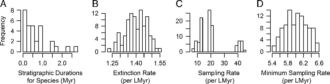
Figure 1 Estimating sampling and extinction rates from the pruned occurrence data. Frequency distributions of stratigraphic durations from 100 individual CONOP solutions (example from one such run in A) were used to calculate samples of estimated extinction rates (B) and sampling rates (C) via maximum likelihood (Foote Reference Foote1997). The number of first and last appearances of taxa across all sections used in the CONOP analysis provide a minimum number of occurrences, which were used with the duration data to calculate minimum bounds for sampling rate (D) across the 100 CONOP solutions, using a different maximum-likelihood method (Solow and Smith Reference Solow and Smith1997).
A different approach, introduced by Solow and Smith (Reference Solow and Smith1997), uses a maximum-likelihood estimator to calculate the instantaneous sampling rate based on taxon durations and the number of collections (sampling events) in which a taxon was found. As described above, we used the minimum number of collections to obtain estimates of the minimum sampling rate. This method is implemented in the R package paleotree.
Results presented for our calculations of sampling and extinction rates are based on pruned composites consisting only of the 30 pterocephaliid taxa on our pruned cladogram, as our main interest is the sampling and diversification rates of the taxa included in our phylogenetic data set. Thus, all analyses in this paper are for those taxa for which cladistic, stratigraphic, and morphometric data were available. Similar analyses were performed for the entire 163 trilobite species included in the CONOP composites, but rate estimates did not qualitatively differ (see Supplementary Material), suggesting that the selected 30 pterocephaliid species are an unbiased subsample of the larger taxonomic data set.
Applying APT Approaches
Hopkins (Reference Hopkins2013b) presented phylogenetic comparative analyses using a phylogeny scaled under the “equal” algorithm (Table 1), times of observation in units of stratigraphic height, and the root age offset by 1 m. For the absolute timescale used in this study, 1 m is effectively ~0.03 Myr. We expanded this to nine variations of a posteriori time-scaling: (1) a set of trees time-scaled using the minimum-node dating approach; (2–4) trees time-scaled using equal with the root age adjusted backward by 0.03 Myr (i.e., 1 meter), 0.1 Myr, or 0.2 Myr; (5–7) trees time-scaled with the minimum branch length algorithm (MBL), using respectively 0.03 Myr, 0.1 Myr, or 0.2 Myr as the MBL variable; and (8–9) cal3 using the median sampling and extinction rate estimates calculated from the duration frequency analyses (see “Results”), and allowing and disallowing ancestor inference (Bapst Reference Bapst2013a). Each APT approach was applied once for each of the 100 CONOP composites, such that each approach is represented by 100 time-scaled trees. The age of the occurrence selected for each taxon (i.e., the times of observation) can have a significant impact on comparative methods (Bapst Reference Bapst2014). Our goal was to examine how different APT approaches impact the findings of Hopkins (Reference Hopkins2013b), so we followed the protocol used there of time-scaling with the first appearances as the times of observation. The morphological dataset used is the mean shape of the cranidium, averaged across time and space for each species, and may be considered the expected shape of the first representatives of each species. All of these approaches were applied using functions in the R package paleotree (Bapst Reference Bapst2012).
Phylogenetic Comparative Methods for Testing Time-Dependent Rates of Trait Evolution
Hopkins (Reference Hopkins2013b) recovered a negative trend through time in the rate of ancestor–descendant morphological change, using a multivariate approach. These rates were calculated via maximum-likelihood reconstructions of ancestral node values (Schluter et al. Reference Schluter, Price, Mooers and Ludwig1997; as implemented in R package ape [Paradis et al. Reference Paradis, Claude and Strimmer2004]) for all PCs, on a unit-length tree (a phylogeny in which all internode edge lengths are 1), and then dividing the Euclidean distance between the ancestor and descendant PC values for all edges by their respective edge lengths on the time-scaled tree. The correlation between “time” (technically, stratigraphic height) and rate was measured as Kendall’s tau. We applied the exact same protocol for all samples of time-scaled trees, although with the additional step of ignoring any infinite rates estimated when edge lengths were zero (which are impossible under equal or MBL but not MND or cal3, which were not applied in the original study). Alternative analyses in which zero-length branches were not ignored did not produce qualitatively different results (see Supplementary Material for details).
To assess the degree to which similar procedures might produce different results, we conducted two additional tests of the temporal trend in the rate of trait evolution. First, we applied the same ancestor–descendant divergence analysis described above, except with ancestral node values estimated using the time-scaled trees, not a unit-length tree. This avoids possible misestimation of ancestral values due to ignoring temporal structure.
Second, we applied recently developed methods for fitting models of trait evolution to multivariate data sets, provided in the R package mvMorph (Clavel et al. Reference Clavel, Escarguel and Merceron2015). Following best practices recommended by Slater and Pennell (Reference Slater and Pennell2014) for testing for time-dependent change in rates of morphological change, we fit a version of the “early-burst” (EB) model, relaxed to allow either an exponential decrease or increase with time of the rate of morphological change (so, allowing for both late-burst and early-burst scenarios), which is functionally identical to the “accelerating–decelerating” (ACDC) model (Blomberg et al. Reference Blomberg, Garland and Ives2003). The support for an early-burst or late-burst scenario can be summarized using the maximum-likelihood value of the beta parameter returned by the function mvEB, but rather than examining this value in its raw state, we transformed it to the more interpretable number of rate half-lives elapsed over a clade’s evolutionary history, which is T/[log(2)/beta] (Slater and Pennell Reference Slater and Pennell2014), where T is tree depth. Tree depth, however, varies within our samples of examined trees, so instead we used a flat 5 Myr as T (close to the total duration of the pterocephaliids in the fossil record), thus calculating the number of doublings (or halvings) per 5 Myr. Unfortunately, we could not perform this analysis on all 30 PCs, as this was prohibitively slow, so we instead limited our analyses to the first four PCs, which account for more than 95% of the variance in the data set, decreasing our computational time by almost three orders of magnitude. To avoid numerical issues related to zero-length branches in model-fitting comparative analyses, we slightly adjusted terminal edge lengths by 0.001 Myr, following Bapst (Reference Bapst2014).
Testing Ancestor–Descendant Inference
We examined the pattern of ancestor–descendant inferences within an additional set of phylogenies using cal3, with last appearances as the times of observation for the taxon units (i.e., tips will reflect the last appearance times). This was done because the use of first appearances will lead to an underestimation of the frequency of inferred ancestors, as branching of child lineages from taxa later in their duration may be inappropriately down-weighted by the cal3 algorithm. While putative ancestors are tagged as such in the output of cal3 (as well as by evolutionary mode; i.e., anagenesis or cladogenesis), descendants are not tagged as such, because cal3 only recognizes one sister lineage as the descendant, but this may be a single taxon or a very large clade containing many taxa. The actual identity of the descendant in the latter case is somewhat amorphous, but the most probable identity is that of the earliest appearing taxon in that clade. We use this guideline to identify the descendant taxon for each inferred ancestor.
All data, input files and programming scripts for recreating all analyses and figures can be found at Dryad repository http://datadryad.org/handle/10255/dryad.122995.
Empirical Case Study: Results
Estimates of Sampling and Diversification Rates
As trilobites are a group of marine invertebrates with a rich fossil record, a number of previous estimates for sampling rate already exist in the literature, at a range of taxonomic, temporal, and geographic scales (Table 2). These estimates can have a correspondingly large degree of variability across those scales, with a global Phanerozoic-scale study of genera reporting 0.19–0.39 per lineage million years (per LMyr; Foote and Sepkoski Reference Foote and Sepkoski1999), while the sampling rate estimate from a single locality in Oklahoma has an apparent sampling rate of 17.46 per LMyr (Foote and Raup Reference Foote and Raup1996). This last value is exceedingly high, suggesting that the trilobite record might be very complete at small spatial scales.
Our maximum-likelihood estimates of sampling rate showed considerable variation (more than 30 units per LMyr), especially compared with the much narrower distribution of extinction rate estimates (Fig. 1B,C). The median sampling rate from our pruned data set was 19.07 per LMyr, and the median extinction rate was 1.40 per LMyr. The minimum sampling rate estimates (following Solow and Smith Reference Solow and Smith1997) were much more constrained than the estimates from the range frequency distributions (Fig. 1D), with a median of 6.02 per LMyr.
Overall, these calculations suggest that the record of the pterocephaliid trilobites within the Great Basin is extremely complete and well-sampled, comparable to the sampling estimates from Foote and Raup (Reference Foote and Raup1996) based on a single section of upper Cambrian–Ordovician trilobites from Oklahoma (Table 2). Although the cross-validation of the high sampling rates estimated from the range frequencies versus the high minimum-rate estimates is reassuring, it is important to evaluate the realism of these rates based on estimates in other groups and their implications for taxonomic completeness and turnover. For example, the median sampling and extinction rate estimates would imply an average species duration of 0.71 Myr and an average waiting time between sampling events (collections) for a single species within its duration of 0.05 Myr, and given those values, that the average species will be collected at 13 horizons over its duration. Although we have only limited information on the number of collections a taxon was sampled at, the average minimum number of horizons a taxon occurred at was 5.8, which would be consistent with the above estimate. The mean average duration of a species in our pruned data set was 0.66 Myr, which also matches well with our parameter estimates. We can also use these rate estimates to calculate taxonomic completeness: the probability of sampling a taxon at least once, equivalent to the expected proportion of taxa that were observed (Foote and Raup Reference Foote and Raup1996). The expected taxonomic completeness for this data set is 0.93, implying that the pterocephaliid record is exceedingly complete but that some fraction of species may still have been unsampled. Overall, the median sampling (19.07 per LMyr) and extinction (1.40 per LMyr) rate estimates imply nothing that seems unlikely a priori in comparison to what we know of the pterocephaliid record and the fossil record of other groups, and thus we adopt these as valid estimates for use in cal3. We choose to use median values rather than sampling from our sample of rate estimates, as the resulting distributions are multimodal, with extreme outliers likely due to outlier sets of CONOP ranges. Additionally, as the pterocephaliids are extinct (and their entire evolutionary history is captured here, with taxa only omitted due to missing character or stratigraphic information), the long-term branching rate must equal the extinction rate, and thus we use the median extinction rate as an estimate of the branching rate.
Comparing Divergence Dates on Time-Scaled Trees
While there are a variety of ways for sets of time-scaled trees to differ (Bapst Reference Bapst2014), one simple way to visualize their effect on divergence dates is to calculate the distribution of node ages and visualize these on a common absolute timescale. We do this both for the root divergence of the tree (the split between Aphelaspis haguei and the other 29 pterocephaliid species) and a more derived node, in this case the split between the sister genera Sigmocheilus and Pterocephalia (Fig. 2). Little variation is seen among the root divergence dates, except that the minimum branch length algorithm shifts the root age back about 1 Myr, suggesting many of the edge lengths may be considerably less than 0.2 Myr. The slight variation among sets of trees time-scaled with equal matches the difference in their root age offset values. More variation is seen in the age estimates of the more nested node, with a linear difference in node ages observed as minimum branch length is increased. The three equal method treatments estimated the same divergence date for the Sigmocheilus–Pterocephalia split, which agrees with the description of the underlying algorithm (Bell and Lloyd Reference Bell and Lloyd2015), as node ages should only be influenced by the root age’s offset if they are part of an unbroken chain of zero-length edges leading to the root, meaning that the divergence dates of more derived nodes are likely to stay the same as the root age offset changes, unlike more root-ward divergences. For both of these node age comparisons, cal3 implies node age distributions that are very similar to the MND approach.
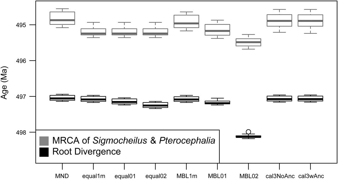
Figure 2 Variation in selected divergence dates under different a posteriori time-scaling approaches. Box plots reflect the distribution of ages for the root node and a nested node that represents the most recent common ancestor (MRCA)of the genera Sigmocheilus and Pterocephalia, calculated across 100 sets of stratigraphic ranges, reflecting different CONOP solutions. For the time-scaling approaches listed, MND represents minimum-node dating. The “equal1m,” “equal01,” and “equal02” labels represent the equal branch-sharing approach (Brusatte et al. Reference Brusatte, Benton, Ruta and Lloyd2008) with the root age adjusted by 1 m of stratigraphic height (i.e., 0.03 Myr), 0.1 Myr, and 0.2 Myr, respectively. The “MBL1m,” “MBL01,” and “MBL02” labels represent the minimum branch length approach (Laurin Reference Laurin2004) using minimum lengths of 0.03 Myr, 0.1 Myr, and 0.2 Myr, respectively. See Table 1 for further description of these approaches. The right-most labels, “cal3NoAnc” and “cal3wAnc,” represent the cal3 approach, variously disallowing or allowing for the cal3 algorithm to infer observed taxa as direct ancestors (Bapst Reference Bapst2013a).
Comparing Support for Early-burst Trait Evolution on Time-Scaled Trees
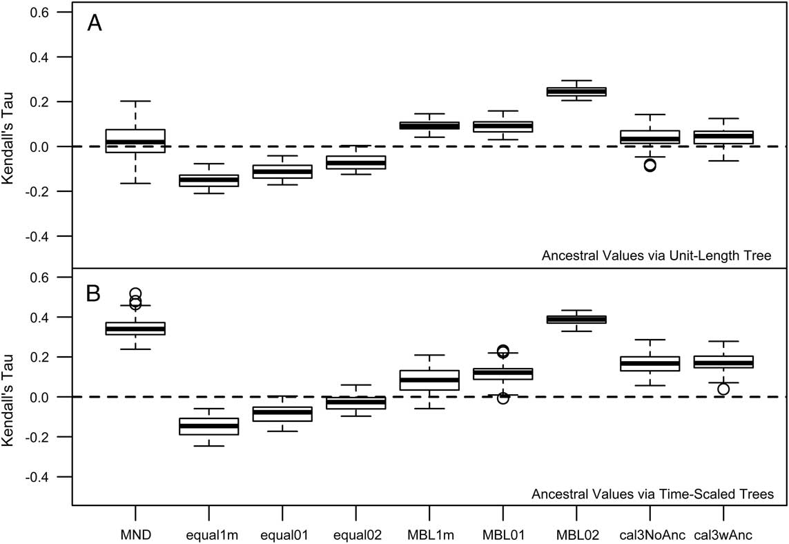
Hopkins (Reference Hopkins2013a) reported a “triangle-shaped” association between time and rate of morphological evolution in the pterocephaliids, such that rates were highly variable early on, with the maximum rate decreasing through time. As a result, the original reported correlation was not particularly high (Kendall’s tau=−0.24). This value is only slightly more negative than correlation estimates from trees time-scaled the same way (equal, root offset of 1 m) reported herein (Fig. 3A), suggesting that our methodology is consistent with Hopkins’s previous protocol (any difference is due to the different range composites used). However, the sign and strength of the correlation is highly dependent on the time-scaling method (Fig. 3A). Over all samples, MND and cal3 tend toward zero correlation, equal time-scaling tends to suggest negative correlations, and MBL implies positive correlations. In addition, while the relative difference in correlations mainly stays the same when time-scaled trees instead of a unit-length tree are used for ancestral trait reconstruction (Fig. 3B), all tree samples shift at least marginally toward more positive correlations (i.e., more support for a late-burst scenario), implying that the new ancestral reconstructions imply more trait change on later rather than earlier branches. The largest shift in correlation coefficient occurs with minimum-dated trees: this likely reflects the effect that zero-length time-scaled edges are having on the ancestral trait reconstruction, as they are only removed postreconstruction.

Figure 3 Kendall’s tau correlations of the rate ancestor–descendant change (across all PCs) versus node age. Node age was negated, such that positive correlations represent rates increasing with time (late burst) and negative correlations reflect rates decreasing with time (early burst). There were some differences among estimates depending on whether ancestral trait reconstruction was done on a phylogeny in which all edge lengths were scaled to 1 (A) or on the time-scaled tree used for other components of the rate calculation (B). See the caption for Fig. 2 for information on the respective time-scaling approaches.
Model-fitting analyses also show weak to moderate support for either early-burst or late-burst scenarios, but some dating methods gave contradictory inferences relative to those from the ancestor–descendant contrast analyses (Fig. 4). In particular, the MND and cal3 approaches suggested late-burst dynamics using ancestor–descendant contrasts on dated trees, but early-burst dynamics when model-fitting analyses were applied. While MND trees imply a wide degree of uncertainty for either scenario, other methods imply between one to two doublings and/or halvings of the evolutionary rate over 5 Myr, with that envelope of uncertainty being largest under cal3, which weakly supports an early-burst scenario.
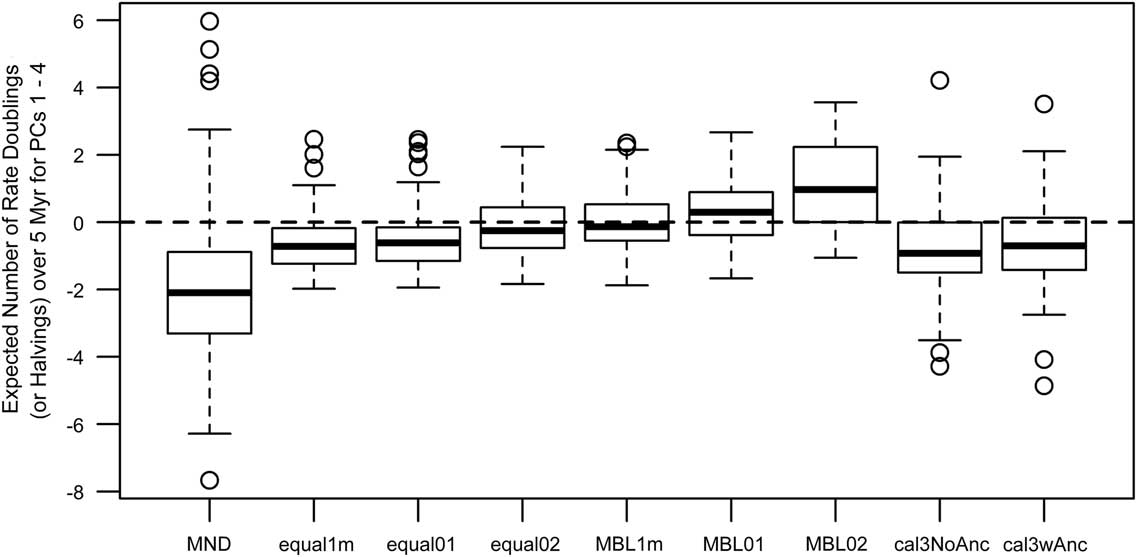
Figure 4 Estimates of time-dependent change in the rates of trait evolution (across PCs 1–4) using multivariate model-fitting analyses from R package mvMORPH (Clavel et al. Reference Clavel, Escarguel and Merceron2015). The summary statistics shown are based on estimated model parameters (Slater and Pennell Reference Slater and Pennell2014) and represent, if positive, the expected number of doublings of rate expected over 5 million years, indicating that the rate of trait evolution has increased over time (late burst). If negative, the values represent the expected number of halvings of rate over 5 Myr, indicating that the rate of trait evolution has decreased over time (early burst). See the caption for Fig. 2 for information on the respective time-scaling approaches.
Inferring Ancestor–Descendant Relationships with cal3
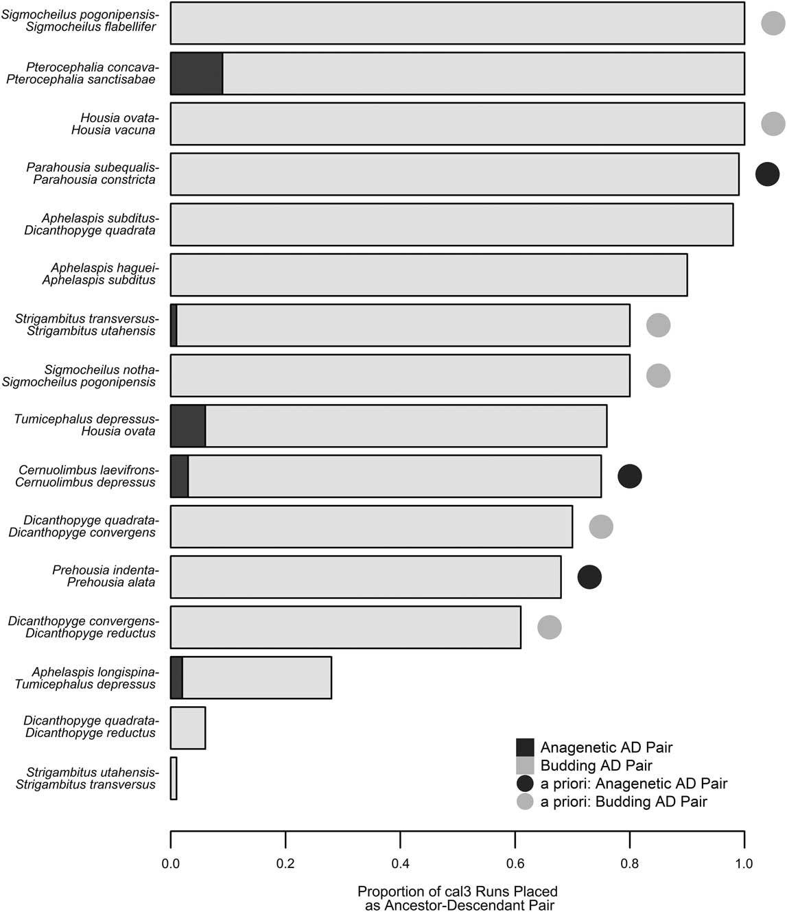
Based on tree topology, stratigraphic distribution, and optimized character state transformations, Hopkins (Reference Hopkins2011a) named nine potential ancestor–descendant pairs in the pterocephaliids, including six budding cladogenetic pairs (in which a morphologically distinguishable daughter species appears via branching from some persistent ancestral species) and three anagenetic pairs (in which one morphologically defined species evolves, without branching, into another morphospecies). We recovered 16 potential ancestor–descendant pairs across 100 trees generated using cal3 and last appearance dates, with each tree containing 8 to 14 of these pairs. Thirteen pairs were found across more than 60% of the cal3 trees (Fig. 5), which includes all nine a priori pairs listed by Hopkins (Reference Hopkins2011b). However, anagenesis was rarely inferred for any species pair, even for those previously supposed to represent anagenesis. Almost all inferred ancestors were placed as ancestor to a single descendant taxon, reflecting that cal3 is very constrained by the cladogram used, which lacks polytomies, and thus any given taxon can only be ancestral to its respective sister taxon. The only variation that occurs is when there is variation in the order of appearance of taxa across CONOP solutions. For example, Dicanthopyge quadrata is listed as an ancestor to both D. reductus and D. convergens, depending on which taxon is assigned an earlier first appearance time in a composite section. Similarly, whether Strigambitus utahensis is an ancestor to St. transversus or vice versa depends on which is assigned an earlier first appearance time.

Figure 5 Comparison of inferred ancestor–descendant pairs via cal3 with a priori expectations. The proportion of cal3 time-scaled trees that included a particular ancestor–descendant pair is listed as a stacked bar plot, with the evolutionary mode (anagenesis or budding cladogenesis; Foote Reference Foote1996) indicated by color (dark gray or light gray, respectively). Pairs expected based on previous systematic work (Hopkins Reference Hopkins2011b) are denoted by a circle adjacent to the respective bar, with identical color coding for each evolutionary model.
Discussion
The cal3 time-scaling method requires estimates of diversification and sampling that may, at first glance, seem difficult to estimate. The structure of paleontological data sets can vary greatly, and this makes it difficult to prescribe any simple cookbook procedure for obtaining such estimates. Here, we have obtained meaningful estimates from a data set with qualities that made estimation less than straightforward by taking multiple analytical approaches (Fig. 1) and through careful comparison to previous published estimates. By applying cal3 and other time-scaling methods to this data set, we find that choice of time-scaling method can impact the estimates of divergence dates (Fig. 2) and downstream macroevolutionary analyses (Figs. 3, 4). The cal3 approach also allows us to consider the potential for sampled ancestors in our data set, which is not offered by any other APT approach (Fig. 5). Furthermore, as the results of analyses from multiple MPT and branch-sharing analyses did not always include the results of the cal3 analyses, it may be inadequate to test for sensitivity to dating error by using various arbitrary APT approaches with a range of constants (e.g., Betancur-R et al. Reference Betancur-R, Ortí and Pyron2015; Bates et al. Reference Bates, Mannion, Falkingham, Brusatte, Hutchinson, Otero, Sellers, Sullivan, Stevens and Allen2016).
Furthermore, the varying results of the analyses we applied to test for early bursts of rapid trait evolution in the pterocephaliids were not due only to varying time-scaling methods, but also to the specific approach used to analyze trait evolution. In particular, trees dated with cal3 predicted a weak late-burst pattern using the ancestor-reconstruction approach, but a weak early-burst pattern using the model-fitting approach. Ancestral reconstructions of continuous traits are often avoided by evolutionary biologists because of their wide confidence intervals, suggesting a high degree of uncertainty (Schluter et al. Reference Schluter, Price, Mooers and Ludwig1997; Losos Reference Losos2011). Although it has been shown that fossils can improve the accuracy of reconstructed trait values (Finarelli and Flynn Reference Finarelli and Flynn2006), there is as yet no evidence that fossils improve precision to such a degree that they become usable for testing macroevolutionary patterns (contra Alroy Reference Alroy2000), despite their wide use in paleobiology (Butler and Goswami Reference Butler and Goswami2008; Zanno and Mackovicky Reference Zanno and Makovicky2013; Hopkins Reference Hopkins2016). In this case, there is no way to determine which analytical approach is more accurate, and regardless of the evolutionary interpretation of directionality, the difference in effect size from time-constant rates is relatively small. We recommend that paleontologists using phylogenetic comparative methods to test macroevolutionary hypotheses should always explore multiple approaches.
The cal3 approach can infer ancestor–descendant pairs and categorizes these between anagenetic and budding cladogenetic relationships, and it may help unlock the extent to which branching events are integral to how morphotaxa “speciate” (morphologically differentiate) from one another (Wagner and Erwin Reference Wagner and Erwin1995; Ezard et al. Reference Ezard, Pearson, Aze and Purvis2012; Bapst Reference Bapst2013b; Pennell et al. Reference Pennell, Harmon and Uyeda2014). However, the cal3 determination is independent of character data and is based solely on stratigraphic ranges and tree topology. Tip-dating methods can also place ancestors, but only as sampled ancestral populations assigned to a specific point in time (Gavryushkina et al. Reference Gavryushkina, Welch, Stadler and Drummond2014; Heath et al. Reference Heath, Huelsenbeck and Stadler2014), and thus cannot distinguish modes, while stratocladistic methods can infer mode but are not based on an explicit probabilistic model (Fisher Reference Fisher2008). The ancestor–descendant pairs inferred by cal3 and presumed a priori match fairly well, suggesting that cal3 ancestor inference is congruent with qualitative assessments of ancestral relationships. The only seeming discordance is the low observation of anagenetic ancestors, given that two of the anagenetic pairs proposed by Hopkins (Reference Hopkins2011b) have simultaneous last appearance dates of the ancestor and first appearance dates of the descendant in the majority of our 100 range composites. However, distinguishing between inferred anagenetic and cladogenetic pairs does not directly equate to the true proportion of anagenesis to cladogenesis. Some “apparent” anagenetic relationships are likely cladogenetic. Anagenesis might be more apparent than real when a taxon at its last appearance time is inferred to be in a direct line of ancestry to one or more sampled taxa, as this pattern would also be observed where branching (i.e., budding or bifurcating cladogenesis; Foote Reference Foote1996) occurs after that last appearance. Any case in which sister taxon ranges do not overlap could potentially be a case of apparent anagenesis (but see Ezard et al. Reference Ezard, Pearson, Aze and Purvis2012 for a contrarian view), with no further grounds to confirm or reject the pattern of differentiation between a particular pair of taxa. This effect is asymmetrical: apparent budding cladogenesis supports only budding cladogenesis, not anagenesis or bifurcation. Thus, there should be an expectation that a number of budding or bifurcating cladogenetic events are mistakenly categorized as anagenesis in any incompletely sampled fossil record. Less than 2% of the ancestor–descendant relationships were categorized as apparent anagenesis, which might be consistent with morphospecies originating only via budding cladogenesis, not true anagenesis or bifurcating cladogenesis. Such a scenario would agree with previous estimates (Wagner and Erwin Reference Wagner and Erwin1995). As current tip-dating approaches only treat taxon units as instantaneous populations, they are not able to differentiate between budding and anagenetic relationships, and thus this sort of analysis is currently possible only with cal3.
Summary
Obtaining accurate, dated phylogenies for fossil taxa is a major objective of modern paleontological systematics. Development of new methods has accelerated in recent years and will probably continue to accelerate for some time into the future. The invention of new probabilistic APT methods, like cal3 (Bapst Reference Bapst2013a), and sampled-ancestor tip-dating (Gavryushkina et al. Reference Gavryushkina, Welch, Stadler and Drummond2014; Zhang et al. Reference Zhang, Stadler, Klopfstein, Heath and Ronquist2016) allows workers to avoid arbitrary time-scaling approaches. Eventually, APT approaches may be replaced by Bayesian tip-dating with fixed topologies and no character data, as already seen in some vertebrate paleobiology studies (e.g., Close et al. Reference Close, Friedman, Lloyd and Benson2015; Fischer et al. Reference Fischer, Bardet, Benson, Arkhangelsky and Friedman2016), in which taxa are known from a small number of dated collections. Despite these methodological advances, the simpler APT approaches remain in common use, even though it is clear from both previous simulations (Bapst Reference Bapst2014) and empirical case studies (such as this paper) that those approaches provide results that differ from statistically valid time-scaling approaches. We show here that it is possible to get useful estimates of sampling, branching, and extinction rates for cal3 and that it is worth the effort. A dated phylogeny of fossil taxa is a complex product that can have considerable influence on the macroevolutionary inferences made from it. Dated phylogenies of fossil taxa also offer immediate opportunities to compare the estimated divergence dates with the timing of stratigraphic appearances and paleoenvironmental changes and the potential to explore ancestor–descendant relationships. The steps taken to date fossil phylogenies warrant more attention in the literature, and empirical studies whose main aim is to produce dated phylogenies should be viewed as important and worthy stand-alone contributions to paleontological systematics.
Acknowledgments
We thank G. Slater for advice on comparing the fit of early-burst models, and P. Sadler for discussion about using CONOP output for this particular application. We thank G. Hunt, W. Kiessling, and an anonymous reviewer for comments. D.W.B. was supported by National Science Foundation grant EAR-1147537 to S. Carlson.
Supplementary Material
Data available from the Dryad Digital Repository: http://dx.doi.org/10.5061/dryad.292dd