


Introduction
Anthropogenic climate change can induce regional extirpations and global extinctions (Cahill et al. Reference Cahill, Aiello-Lammens, Fisher-Reid, Hua, Karanewsky, Yeong Ryu, Sbeglia, Spagnolo, Waldron, Warsi and Wiens2012), which are expected to be most severe in the tropics (Vamosi and Vamosi Reference Vamosi and Vamosi2008; Nguyen et al. Reference Nguyen, Morley, Lai, Clark, Tan, Bates and Peck2011; Doney et al. Reference Doney, Ruckelshaus, Emmett Duffy, Barry, Chan, English, Galindo, Grebmeier, Hollowed, Knowlton, Polovina, Rabalais, Sydeman and Talley2012). In the past, climate change caused by massive volcanism had an important role in several extinction crises (Kiessling and Simpson Reference Kiessling and Simpson2011; Bond and Grasby Reference Bond and Grasby2017). Then as now, climate change acted on marine life by combined rapid warming, anoxia, and acidification (climate-related stressors, “CRS” hereafter), the ecological importance of which varies by geography and phylogeny (Pörtner and Langenbuch Reference Pörtner and Langenbuch2005; Breitburg et al. Reference Breitburg, Levin, Oschlies, Grégoire, Chavez, Conley, Garçon, Gilbert, Gutiérrez, Isensee, Jacinto, Limburg, Montes, Naqvi, Pitcher, Rabalais, Roman, Rose, Seibel, Telszewski, Yasuhara and Zhang2018). Taxonomic, environmental, and geographic variation in extinctions may thus provide ecological signatures to CRS responses (Payne and Finnegan Reference Payne and Finnegan2007; Kiessling and Simpson Reference Kiessling and Simpson2011; Finnegan et al. Reference Finnegan, Anderson, Harnik, Simpson, Tittensor, Byrnes, Finkel, Lindberg, Liow, Lockwood, Lotze, McClain, McGuire, O'Dea and Pandolfi2015). One potential signature is the significant departure from a globally homogenous extinction rate, instead selecting one latitudinal band over another, which we term latitudinal extinction selectivity (LES). LES has received some attention for individual intervals (Kiessling and Aberhan Reference Kiessling and Aberhan2007; Kiessling et al. Reference Kiessling, Aberhan, Brenneis and Wagner2007; Vilhena et al. Reference Vilhena, Harris, Bergstrom, Maliska, Ward, Sidor, Strömberg and Wilson2013), but the dependency of LES on the changing global environment is untested. We summon the marine fossil record to test the generality of relatively greater tropical than temperate extinctions in response to climate warming pulses over the past 450 Myr.
Generalizations about the environmental triggers of past extinction risk can be projected to modern clades (Harnik et al. Reference Harnik, Lotze, Anderson, Finkel, Finnegan, Lindberg, Liow, Lockwood, McClain, McGuire, O'Dea, Pandolfi, Simpson and Tittensor2012; Finnegan et al. Reference Finnegan, Anderson, Harnik, Simpson, Tittensor, Byrnes, Finkel, Lindberg, Liow, Lockwood, Lotze, McClain, McGuire, O'Dea and Pandolfi2015). Organism traits such as skeletal mineralogy and physiological plasticity (sometimes called “buffering”) are linked to vulnerabilities to CRS at Phanerozoic scales (Bambach et al. Reference Bambach, Knoll and Sepkoski2002; Kiessling et al. Reference Kiessling, Aberhan and Villier2008; Kiessling and Simpson Reference Kiessling and Simpson2011). Higher tropical extinction risk was previously observed during the end-Triassic (Kiessling and Aberhan Reference Kiessling and Aberhan2007) and end-Cretaceous (Vilhena et al. Reference Vilhena, Harris, Bergstrom, Maliska, Ward, Sidor, Strömberg and Wilson2013) mass extinctions, suggesting a trigger role for climate change. Meanwhile, Jurassic and Triassic background extinction intervals showed no significant LES (Kiessling and Aberhan Reference Kiessling and Aberhan2007; Kiessling et al. Reference Kiessling, Aberhan, Brenneis and Wagner2007), with mass extinction intervals defined over background as the significant outliers (Raup and Sepkoski Reference Raup and Sepkoski1982). The consistency of LES over intervals of different extinction rates is yet untested, but some studies suggest that the tropics may have generally higher extinction rates (Vamosi and Vamosi Reference Vamosi and Vamosi2008; Powell et al. Reference Powell, Moore and Smith2015). Still, controlled experiments and high–spatiotemporal resolution observations of CRS responses of modern organisms may be key to understanding the mechanisms underlying LES.
Global warming may be linked to LES through organismal physiology. Phylogenetically constrained differences in oxygen and capacity-limited thermal tolerance (Pörtner and Langenbuch Reference Pörtner and Langenbuch2005; Bozinovic and Pörtner Reference Bozinovic and Pörtner2015) may be responsible for the profound differences in extinction proneness among clades (Raup and Boyajian Reference Raup and Boyajian1988; Finnegan et al. Reference Finnegan, Anderson, Harnik, Simpson, Tittensor, Byrnes, Finkel, Lindberg, Liow, Lockwood, Lotze, McClain, McGuire, O'Dea and Pandolfi2015). Extinctions may also appear indiscriminate because of confounding factors or because of hard biological limits to temperature, oxygen levels, or habitat (Song et al. Reference Song, Wignall, Chu, Tong, Sun, Song, He and Tian2014; Storch et al. Reference Storch, Menzel, Frickenhaus and Pörtner2014). However, these physiological limits are closest in the tropics (Nguyen et al. Reference Nguyen, Morley, Lai, Clark, Tan, Bates and Peck2011). When organisms meet their limits, range shifts are expected (Kiessling et al. Reference Kiessling, Simpson, Beck, Mewis and Pandolfi2012; Reddin et al. Reference Reddin, Kocsis and Kiessling2018), but rapid rates of environmental change may also force widespread extinctions. Indeed, current climate velocities are greatest in the tropics, making these regions prone to extirpations (Burrows et al. Reference Burrows, Schoeman, Richardson, Molinos, Hoffmann, Buckley, Moore, Brown, Bruno, Duarte, Halpern, Hoegh-Guldberg, Kappel, Kiessling, O'Connor, Pandolfi, Parmesan, Sydeman, Ferrier, Williams, Poloczanska, O'Connor, Pandolfi, Parmesan, Sydeman, Ferrier, Williams and Poloczanska2014). Doney et al. (Reference Doney, Ruckelshaus, Emmett Duffy, Barry, Chan, English, Galindo, Grebmeier, Hollowed, Knowlton, Polovina, Rabalais, Sydeman and Talley2012) cite warming-related disruption to the sensitive coral–algal symbiosis as another likely cause for elevated tropical extinctions, but also elevated polar extinctions due to sea-ice retreat and migrations. Stanley (Reference Stanley1987) originally proposed a poleward migration dead end to follow long-term warming and, conversely, that equatorward migrations following cooling might cause tropical extinctions. Although this idea importantly hypothesizes a link between extinctions and Earth-surface geometric constraints, paleo-polar regions are typically not well sampled, such that we contrast only tropical and temperate LES.
We test two alternatives against the null hypothesis that observed LES results from sampling patterns. (1) General tropical LES irrespective of overall extinction rate. This is a special form of the hypothesis that the tropics are cradles but not museums of biodiversity (Kiessling et al. Reference Kiessling, Simpson and Foote2010). (2) The tropics are most vulnerable during extinction crises, because of rapid warming and deoxygenation. In particular, tropical selectivity should arise at the end-Permian (Changhsingian) and end-Triassic (Rhaetian) mass extinctions, which are deemed similar in causation and patterns and were accompanied by massive global warming (Kiessling and Simpson Reference Kiessling and Simpson2011; Van De Schootbrugge and Wignall Reference Van De Schootbrugge and Wignall2016). Where possible, we try to correlate observed LES with proposed climatic or other potential environmental causes. We approximate interval average temperatures by stable oxygen isotopes of fossils, and pulsed climatic events by the dominant view in the literature, which generally follows high–temporal resolution stratigraphic studies (Table 1).
Table 1. Biotic crisis intervals with pulsed climatic events. Supplementary details on potential causal mechanisms are either from Table 1 in Bond and Grasby (Reference Bond and Grasby2017) or Table 2 in Kiessling and Simpson (Reference Kiessling and Simpson2011). CAMP, Central Atlantic Magmatic Province; LIP, large igneous province; NAIP, North Atlantic Igneous Province; OA, ocean acidification; PETM, Paleocene–Eocene thermal maximum; PPD, Pripyat-Dnieper-Donets rift.

Table 2. Per capita (PC) extinction rates of tropical- and temperate-affinity genera. Geological time intervals exhibiting at least weak evidence (L ≥ 60% likelihood) of LES are shown. Extinction crisis interval names are in bold type. Percent (%) likelihood is the normalized probability, converted from Akaike weights, of a dual-rate over a single-rate model, with moderate evidence (L ≥ 80%) in bold type. The log ratio is of tropical:temperate extinction rates, with negative ratios showing relatively higher temperate rates. One rate is twice as high as the other at log ratio ± 0.69. Likelihood for a single rate model is 100 – L dual rate. Per capita rates are after sampling standardization to 600 occurrences iterated 100 times.
O, Ordovician; S, Silurian; D, Devonian; C, Carboniferous; P, Permian; Tr, Triassic; J, Jurassic; K, Cretaceous; Pg, Paleogene; N, Neogene.

Methods
Fossil Occurrences
We accessed the Paleobiology Database (http://www.paleobiodb.org) on 18 December 2017 for marine occurrences at global scales across the post-Cambrian Phanerozoic, numbering 453,000 occurrences after data-cleaning steps (Supplementary Appendix). To focus only on confident taxonomic identifications, we included only marine fossils identified with certainty to the species level. However, we assess genus-level extinction patterns, which are usual for Phanerozoic-scale analyses, because species-level taxonomy of fossils is often uncertain and prone to monographic bias (Valentine Reference Valentine1974). Subgenus names were raised to genus status. We removed duplicate genus occurrences per collection, occurrences without phylum or class attributes, and spiders, insects, higher vertebrate, and terrestrial plant classes (full list in Supplementary Appendix). Occurrence age estimates were binned to stages (Gradstein et al. Reference Gradstein, Ogg, Schmitz and Ogg2012), either based on their age estimate midpoints (low priority) or a provided confirmation of stage name (highest priority, 60% of finished data set). Those with age uncertainty greater than the longest stage, 19.5 Myr, were omitted. Some stages were split more finely based on a minimum number of occurrences and their spread within the stage (substage n ≥ 600, minimum met for multiple million-year bins; Supplementary Table S1). These were between the Permian and Jurassic, when extinction rates were elevated, and within three stages of the Ordovician that had relatively high numbers of occurrences (details in Supplementary Table S1). The Hettangian stage was merged with the Sinemurian 1 (first of two substage intervals) because of a low number of occurrences (n ≈ 350). The advantages of splitting stages include a higher temporal resolution, more statistical degrees of freedom, and a reduction in the placement of interval boundaries at extinction events. Rerunning analyses at the stage level or with different binning procedures did not change the results (Supplementary Appendix, Supplementary Figs. S2 and S3). Occurrence paleo-coordinates were calculated based on the GPlates plate tectonic model (Wright et al. Reference Wright, Zahirovic, Müller and Seton2013), and we use absolute latitudes throughout the study.
Interval average temperature was based on oxygen stable isotopes of well-preserved calcareous shells from the Phanerozoic data set of Veizer and Prokoph (Reference Veizer and Prokoph2015). To avoid conflating temporal and environmental variation, we filtered samples to be from surface waters (mixed layers <300 m deep) of mostly tropical and subtropical zones (“temperate” records retained for the Jurassic period to the Barremian age, when these records dominate). Following Veizer and Prokoph (Reference Veizer and Prokoph2015), the oxygen isotope time series was detrended using Eq. (2) therein and binned to the intervals introduced earlier, and interval medians were calculated. Interval values were transformed into temperature estimates using the transfer function of Visser et al. (Reference Visser, Thunell and Stott2003), assuming the present day δ18O value of 0‰ standard mean ocean water for seawater. Missing isotope values for the Induan stage were interpolated from neighboring interval medians. Oxygen stable isotopes are certainly not a perfect proxy for seawater temperature, because fractionation is also affected by global ice volume, diagenesis, seawater pH, and salinity. While steps have been taken to minimize the effect of some of these sources (Veizer and Prokoph Reference Veizer and Prokoph2015), the likelihood is that they do contribute to the time series, which must be considered when examining our results. Continental shelf area from the maps of Golonka (Reference Golonka, Kiessling, Flügel and Golonka2002) was binned by absolute latitude into tropical and nontropical (see “Data Analysis” for definition). We interpolated these two areal time series to our intervals by local first-degree polynomial regression with automatic smoothing parameter selection (function loess.as() in package ‘fANCOVA’; Wang Reference Wang2010). Environmental changes are the variable first differences, from interval i − 1 into interval i.
Data Analysis
The analytical pipeline begins with the definition of a tropical/temperate threshold and is followed by genus tropical/temperate-affinity testing, tropical/temperate extinction rate calculations with subsampling, and selective/nonselective model selection and ends with analyses of time series.
The first stage in defining LES was to adopt a split between two latitudinal bands. A threshold of absolute 30° latitude was used by Kiessling and Aberhan (Reference Kiessling and Aberhan2007) and concurs with past diversity peaks, which are understood to occupy between 30° and 40° (north and south; Powell Reference Powell2009; Chaudhary et al. Reference Chaudhary, Saeedi and Costello2016). It also concurs with geological indicators of past tropical zones (Ziegler et al. Reference Ziegler, Eshel, McAllister Rees, Rothfus, Rowley and Sunderlin2003) and approximates the post-Cambrian Phanerozoic occurrence median (|29°|). Therefore, latitudes 0–30° are here termed “tropical,” while latitudes >30° are termed “temperate.”
The second stage is to determine a priori which genera have a strong affinity to these latitudinal bands so that tropical and temperate extinction rates can be unambiguously separated. The individual affinity of each genus was tested following Kiessling and Aberhan (Reference Kiessling, Aberhan, Brenneis and Wagner2007; Kiessling and Simpson Reference Kiessling and Simpson2011; Kiessling and Kocsis Reference Kiessling and Kocsis2015), which uses the overall pattern of occurrences to account for varying sampling conditions. For example, the odds ratio between the number of occurrences of the genus Ostrea representing one latitudinal band, a, and the number of Ostrea occurrences representing another latitudinal band, b, contrasts four numbers of occurrences in:
 $$[ {a_{Ostrea}/( {a_{Ostrea} + b_{Ostrea}} ) } ] /[ {a_{{\rm total}}/( {a_{{\rm total}} + b_{{\rm total}}} ) } ] $$
with a total or b total being occurrences of all genera from the stratigraphic range of Ostrea per latitudinal band. If the numerator is greater, then that indicates affinity for band a, and if the denominator is greater, then affinity for band b is indicated. The significance of these putative affinities was tested with binomial tests with an alpha level of α = 0.1 (Kiessling and Aberhan Reference Kiessling and Aberhan2007). This step results in 36.4% of genera having significant latitudinal affinities. We also tested the effect of varying the static threshold between 15° and 40° (Supplementary Fig. S1) and of using a temporally dynamic threshold adjusted by global temperature time series (Supplementary Table S2, Supplementary Appendix). Results are also compared with those obtained under an affinity α = 1, meaning that the binomial tests are not run, and only the odds ratios are contrasted (Kiessling and Aberhan Reference Kiessling and Aberhan2007). Thus, 100% of genera are designated an affinity based on whether or not the proportion of a genus's occurrences above the threshold is a greater than the proportion for the entire data set (i.e., Eq. 1).
For the third stage, we calculate per capita (PC) extinction rates without normalizing for interval duration (see Foote Reference Foote2005), as
 $$\hat{\,p} = -{\rm ln} [ {Nbt/ ( {Nbt + NbL} ) } ] $$
where Nbt is the number of taxa crossing both the bottom and the top boundaries of the interval, and NbL is the number of taxa that cross only the bottom, following Foote (Reference Foote2000). For comparability among temporal intervals, rates are calculated using 100 iterations of classical rarefaction (Raup Reference Raup1975) to meet an equal threshold number of occurrences (n = 600) per interval. This process results in a pool of 600 occurrences per interval from which extinction rates can be calculated separately for tropical-affinity genera, temperate-affinity genera, and all genera. Thus, we define LES by the log ratio of tropical extinction rates to temperate extinction rates per interval. Latitudinal distributions of occurrences varied by time interval, so we ensured an even latitudinal spread of occurrences per interval by equal subsampling (i.e., 300 occurrences) from above and below the interval occurrence median paleo-latitude (median = 28.6°, 1st and 3rd quartiles = 21.2°, 34.2°). This even subsampling of latitudinal bands per interval utilizes the per interval occurrence latitudinal distributions most effectively. The alternative, subsampling from fixed latitudinal bands (e.g., split at 30° latitude, also Powell et al. [2015]), vastly decreases the maximum subsample threshold, increasing noise in the output. Instead, known temporal variation in interval occurrence median latitudes is better utilized and subsequently incorporated into the time-series regression model (see end of this section). Further relationships between sampling attributes and LES allowed us to highlight time intervals that the method is likely to falsely categorize as latitudinally selective or nonselective in extinctions. These false positives or negatives were diagnosed by the location of the interval close to the distribution edge of one or more sampling attributes (Supplementary Appendix, ”Drivers of LES per Interval”). Second-for-third (2f3) total extinction rates (Alroy Reference Alroy2015) are calculated for comparison with PC rates.
Now that we have extinction rates for tropical, temperate, and all genera per interval (thereby LES itself), the final stage is to calculate the likelihood that evidence represents true LES. We calculated Akaike weights following Kiessling and Simpson (Reference Kiessling and Simpson2011), which assess whether an observed split in extinction rates between two subsets of fossil occurrence data is meaningful, given the total occurrence data, per interval. These are expressed per interval, as the evidence ratio (L, in %) for an LES model, L select, over a no-selectivity (or globally homogenous extinction rate) model, L null, as normalized probability (Wagenmakers and Farrell Reference Wagenmakers and Farrell2004), where L select + L null = 100%. For discussion, an interval must show at least weak evidence for a selectivity model, being 1.5 times more likely than no selectivity, L select = 60%. Similarly, four times and eight times more likely demonstrate moderate and strong evidence, respectively, L select = 80% and L select = 88.9% (Royall Reference Royall, Taper and Lele2004). We repeated these analysis steps (subsampling, tropical, and temperate extinction rate calculations and model selection) 100 times, storing the median values across iterations.
Simple hypotheses involving extinction rate time series were tested with Spearman's rank correlation, with potential causal relationships (e.g., between temperature change and extinction rates) assessed using the generalized differences in each variable (McKinney and Oyen Reference McKinney and Oyen1989) to account for serial autocorrelation. Wilcoxon signed-rank tests were used to compare extinction rates. Rather than define crisis intervals by a fixed extinction rate threshold (e.g., highest 10%), we iteratively examine all possible thresholds. Following Payne and Finnegan (Reference Payne and Finnegan2007; also Clapham and Payne Reference Clapham and Payne2011), we employ multiple logistic (binomial) regression models including genus geographic range and phylogenetic membership (phylum-level, Mollusca split further into classes) as predictors to test the role of other organismic traits in determining extinction risk. The binomial response per genus per interval is of extinction or not, with predictors chosen by stepwise selection based on minimizing the Akaike information criteria (AIC; Burnham and Anderson Reference Burnham and Anderson2003). We expressed genus ranges as the mean subsampled maximum great-circle distances of genus distributions (occurrence subsample n = 600, 100 iterations). Logistic regressions were performed separately for significant tropical- and temperate-affinity genera for each interval.
Finally, the possibility for LES to be driven by a complex suite of sampling and environmental variables was explored by minimizing AIC values in GLS models, using R package ‘nlme’ (Pinheiro et al. Reference Pinheiro, Bates, DebRoy and Sarkar2018). The starting model included time series of the sampling variables (from raw data): occurrence median and maximum latitudes, occurrence latitudinal range, and number of occurrences; and the environmental variables: median temperature and its change, changes in tropical and temperate shelf area separately and in their ratio (temperate:tropical), and overall extinction rate. Significant linear temporal trends were removed from variables by retaining the residuals from linear regressions. Independent variable normality was confirmed by Shapiro-Wilk tests (after either log or square-root transformations). Model selection was initiated with second-order error-autoregressive parameters, but updating the model to the optimal order ultimately removed the autoregressive term. This is supported by Durbin-Watson tests, implemented in the ‘car’ package for R (Fox and Weisberg Reference Fox and Weisberg2011), that showed no lags to hold significant residual serial autocorrelation (minimum p = 0.22, lag = 3, maximum lag tested = 5). Ordinary least-squares regression results, which are identical to those of the optimal GLS (with no time-series process for the errors), are thus shown for simplicity. The assumption of additivity was relaxed in a separate model selection run, initiating with all variables as before, but also including environmental interactions. All analyses and averages exclude the first four and last three time bins because of edge effects that distort the extinction rate (remaining intervals n = 89). All analyses were performed in the R statistical computing environment (R Development Core Team 2018). Analytical code for the core functions noted above is available in the R package ‘divDyn’ (Kocsis et al. Reference Kocsis, Reddin, Alroy and Kiessling2018).
Results
Phanerozoic median rates of tropical and temperate extinctions are not significantly different (medians 0.119 and 0.123, respectively; Wilcoxon signed-rank test V = 1736, p = 0.28). On average, tropical and temperate extinction rates closely resembled the overall rate (tropical Spearman's ρ = 0.86, temperate ρ = 0.83, both p < 0.0001). LES is not restricted to mass extinction intervals. Of 89 intervals, nearly a third show at least weak evidence for LES (L > 60%) and a seventh exhibit moderate evidence, or selectivity >4 times more likely than no selectivity (L > 80%; Fig. 1, Table 2). LES is generally robust to varying definitions of “tropical” and “temperate,” although the precise log ratios and likelihoods of some intervals vary (fixed latitudes of 15–40° or dynamic by median global temperature; details in Supplementary Appendix, Supplementary Fig. S1, Supplementary Table S2).
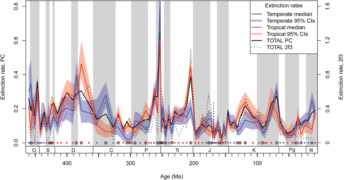
Figure 1. Extinction rate time series for the post-Cambrian Phanerozoic of tropical- and temperate-affinity genera (p < 0.1 affinity for greater or less than 30° latitude, respectively). Polygons (in color online) give the subsampled 95% central intervals after 100 iterations. Per capita (PC) total extinction rate is given by the black line; second-for-third (2f3) total extinction rate (Alroy Reference Alroy2015) is given for comparison, especially at time-series edges (dotted line, right y-axis). Time interval centers are marked by red squares or blue circles (along x = 0) when the tropical or temperate extinction rate is respectively highest. Encircled intervals show at least weak evidence (>60% likelihood) for a dual-rate model being favored, calculated from Akaike weights. Timescale after Gradstein et al. (Reference Gradstein, Ogg, Schmitz and Ogg2012). Alternating background shading shows geological series. Periods are abbreviated along the x-axis: O, Ordovician; S, Silurian; D, Devonian; C, Carboniferous; P, Permian; Tr, Triassic; J, Jurassic; K, Cretaceous; Pg, Paleogene; N, Neogene.
Mass Extinctions and Crises
The Late Ordovician (Katian 2–Hirnantian) mass extinction never exhibits LES despite relatively good sampling coverage and strong tropical shelf gain (Fig. 1, Supplementary Fig. S1). The Late Devonian (Frasnian) and end-Triassic mass extinctions exhibit strong tropical selectivity (L ≈ 96%; Table 2), with strong contributions to Late Devonian LES by tropical cnidarian extinctions (Supplementary Table S3). A Rhaetian temperate extinction of chordates (mostly conodonts) may be of lesser importance. The end-Cretaceous mass extinction (Maastrichtian) shows moderate evidence for temperate extinction selectivity but has a major temperate bias to its occurrences. Further analyses show its LES to be fickle under different approaches (Supplementary Appendix, “Investigating the Maastrichtian”). Logistic regression results with genus affinities by α = 1 suggest a temperate extinction of cephalopods (β = 2.2, p = 0.049), whose latitudinal centroid is significantly temperate-biased relative to the overall centroid (difference in medians = +2.2°, Wilcoxon's W = 30,801, p < 0.0001). The end-Permian and end-Guadalupian (Capitanian) mass extinctions also display LES with a likelihood sensitive to the latitudinal threshold used. However, the direction, temperate selectivity for the end-Permian and tropical for the end-Guadalupian, is not sensitive (Supplementary Appendix, Supplementary Fig. S1). Further analyses support these two intervals’ LES to be valid, including significant contributions by tropical sponges during the end-Guadalupian (see “Discussion”), and temperate brachiopods during the end-Permian (Supplementary Table S3). Tropical selectivity is also supported during the end-Devonian (Famennian) in a warm but cooling climatic state along with major long-term shelf loss (particularly temperate loss), despite a relatively small occurrence range.
Simple Explanatory Models
Elevated extinction intervals show a slight tendency to select tropical genera for extinction, and low extinction intervals to select temperate genera, but this tendency is of weak to marginal significance (Fig. 2A). LES appears unrelated to change in temperature, both during rapid rates of change at mass extinctions and during gradual changes in background intervals (Fig. 2B).
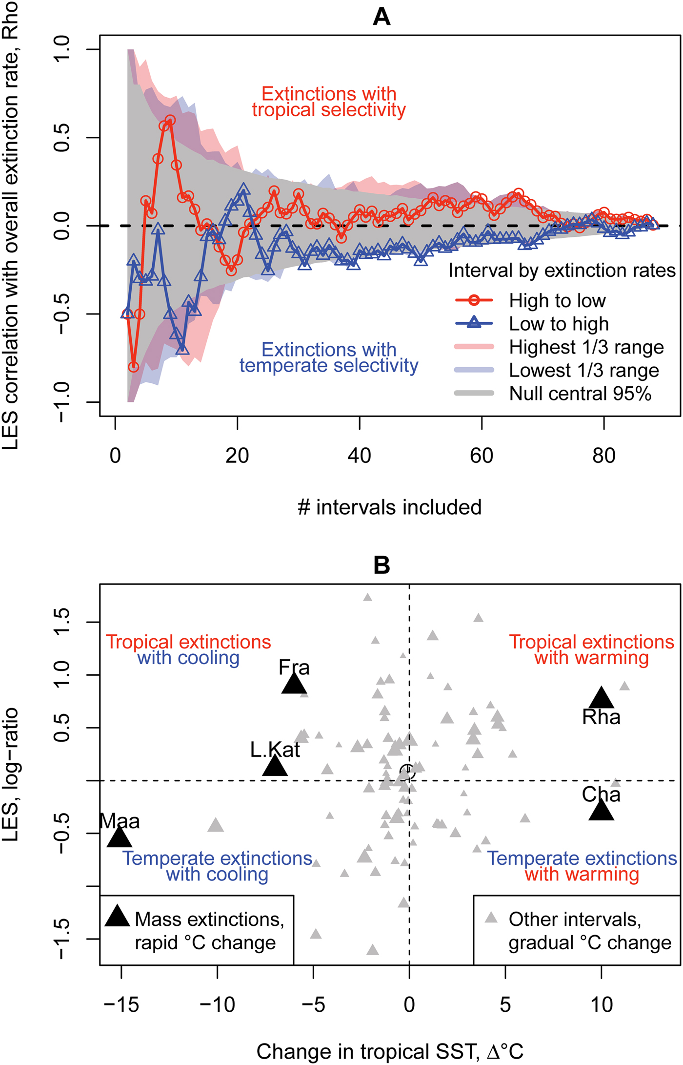
Figure 2. Testing the simple hypotheses that latitudinal extinction selectivity (LES) relates to overall extinction rate or change in temperature. A, Neither high nor low extinction intervals systematically associate with higher tropical or temperate LES. Intervals are ranked by overall extinction rate and iteratively cumulated into the correlations from lowest (triangles), highest (circles), or random order (gray funnel centered on y = 0 is the 95% central interval of 10,000 runs); minimum of three intervals per correlation. Polygons (in color online) are the ranges obtained by varying the starting interval among the upper tercile (red) and lower tercile (blue) of intervals by extinction rate, resuming accumulation by ranked order. B, LES is not simply related to sea-surface temperature (SST) change (ρ = 0.13, p = 0.22; or ρ = 0.15, p = 0.18 with mass extinction interval estimates updated from literature, i.e., black triangle values). Temperature change at mass extinction intervals follows dominant views in the literature (Table 1), while for all other intervals, change in mean temperature was based on low paleo-latitude oxygen isotope data from the Phanerozoic data set of Veizer and Prokoph (Reference Veizer and Prokoph2015). The Kungurian and Cenomanian stages top the warming magnitudes, while the Givetian is the highest magnitude of cooling. Gray symbol size represents interval total extinction rate. Point centroid marked with a crosshair. Intervals with temperature change estimates (Table 1): Cha, Changhsingian; Fra, Frasnian; L.Kat, late Katian; Maa, Maastrichtian; Rha, Rhaetian. LES exhibits no temporal autocorrelation (lag 1 R = 0.05, lag 2 R = 0.1).
Complex Explanatory Models
Bivariate models may be inadequate to explain LES patterns if its driving mechanisms are complex. Model selection settled on an optimal GLS multiple regression model for LES based on combined latitudinal sampling and environmental variables (R 2adj = 0.30; Table 3A). When sampling variables are accounted for, temperate shelf loss associates with temperate selectivity, and warmer climate intervals are more likely to exhibit tropical selectivity (Fig. 3). Another only slightly less well-performing model dropped change in temperate shelf area but instead retained both change in tropical shelf area and the change in ratio of temperate to tropical shelf area, with positive slopes (Table 3). Change in temperate shelf area is strongly correlated with both change in tropical shelf area and change in the temperate to tropical shelf-area ratio (both ρ > 0.65), but the latter two are uncorrelated (ρ = 0.05, p = 0.62). This may indicate that change in temperate shelf area confounds two separate processes that contribute to LES, such as sea-level change and change in relative latitudinal shelf availability. Information for assessing the influence of the occurrence distribution, phylogenetic selectivity, and environmental variables is available for each interval in the Supplementary Appendix (“Drivers of LES per Interval”).

Figure 3. Terms from an optimal time-series multiple-regression model for explaining LES based on environmental (A, B) and sampling (C, D) variables (see also Table 3A). These show the independent contribution (slopes) of each variable (i.e., variation not explained by the other variables), excluding the intercept, so the slope SE dashed lines are straight. Points are the partial residuals, their size representing the overall extinction rate per interval, with the “big five” mass extinctions shaded and labeled (above or below the point). Intervals labeled on Fig. S9. Cap, Capitanian; Cha, Changhsingian; Fam, Famennian; Fra, Frasnian; Hir, Hirnantian; L.Kat, late Katian; Maa, Maastrichtian; Rha, Rhaetian. Occ., occurrence.
Table 3. An optimal model for explaining latitudinal extinction selectivity based on sampling and environmental variables. A, Initial model with additive terms only. Optimal model AIC = 148.6 vs. the full model AIC = 156.8 and a model including only the intercept AIC = 176.9. An alternative model (AIC = 149.8) dropping Δ temperate shelf area instead retains Δ tropical shelf area, slope = 2.1E-07, p = 0.05, and Δ ratio of temperate:tropical shelf area, slope = 12.7, p = 0.001. B, Initial model with additive sampling and multiplicative environmental terms. Model AIC = 140.4, R 2adj = 0.38. Note that adding an interaction term to the optimal additive model does not improve that model. Occ., occurrence.

Relaxing the assumption of additivity to include first-order interaction terms between temperature and shelf-area variables improves the end model (AIC = 140.4, R 2adj = 0.38; Table 3B). Although their main effects remain significant and positive, the link between relative tropical shelf loss and tropically selective extinctions is strongest during moderate to cooler temperatures. During high temperatures, however, the relationship can flip, so that even relative tropical shelf gain, or temperate loss, gives tropical selectivity.
Discussion
The post-Cambrian Phanerozoic LES pattern relates significantly to interval climate state and change in continental shelf area, with warm intervals coinciding with tropical LES and temperate shelf loss coinciding with temperate LES. Our results demonstrate either, or both, of the following. (1) The classic, simplistic assumptions used to interpret LES patterns in the fossil record are naïve. For example, LES appears unrelated to rapid or gradual climate change, calling into question the hypothesis that latitudinal temperature gradients and hemispheric geometry systematically cause a squeeze on habitat space as the climate changes (Stanley Reference Stanley1987). (2) Alternatively, our understanding of global climate through time, and its complicated link to observed extinction rate, is inadequate. These possibilities are explored in the following sections. There is only weak evidence for a higher turnover of tropical genera during elevated extinction rate intervals, and our hypothesis that warming pulses put tropical taxa at higher extinction risk is not clearly supported. Instead, interpretation of an interval's LES pattern should account for the latitudinal sampling and shelf-area distribution.
Phanerozoic Climate History
Although we use the dominant views on climate change over mass extinction events (Table 1), which are the focus of our study, the precise extinction trigger and temporal resolution required to observe its effects are often unknown (see Bond and Grasby Reference Bond and Grasby2017). We expect the rate of climate change to be more important than the magnitude, but rates are systematically underestimated in long time span studies (Kemp et al. Reference Kemp, Eichenseer and Kiessling2015). Furthermore, although oxygen isotopes are a useful proxy of ancient climate, they are far from perfect (see “Methods”), although a suite of additional proxies are typically used to prove climate change over mass extinction events. Thus, our result of no correlation between magnitude of climate change and extinction selectivity may be unsurprising. Even during the warm intervals of the Late Devonian, Early Triassic, and mid- to Late Cretaceous, when it was warm with high sea levels, or during the cold Pennsylvanian to the Cisuralian, no LES tendency is obvious.
Conflicting Patterns
LES is commonly out of line with simple expectations based on climate change, indicating a complex set of drivers. For example, the perhaps dominant view is that the Late Ordovician mass extinction was triggered by massive global cooling in a greenhouse world (Finnegan et al. Reference Finnegan, Heim, Peters and Fischer2012). No global support for LES at this interval could suggest that cooling itself may not produce geographically differential extinction patterns. Finnegan et al. (Reference Finnegan, Heim, Peters and Fischer2012) found some evidence of tropical LES, but that study's focus was confined to North America. However, new evidence argues that changes in redox state may have been as or more important than changes in climate per se (Zou et al. Reference Zou, Qiu, Poulton, Dong, Wang, Chen, Lu, Shi and Tao2018).
The divergence in LES between the end-Permian and end-Triassic mass extinctions is also striking but may be confounded by changes in shelf area (e.g., Rhaetian temperate shelf relative gain or changes beneath our temporal resolution). Both crises were ultimately caused by magmatism and are thought to have been accompanied by similar rates of warming and ocean acidification (Van De Schootbrugge and Wignall Reference Van De Schootbrugge and Wignall2016). Rapid sea-level fall and rise at both boundaries may also indicate brief cooling before longer-term warming at both boundaries (Schoene et al. Reference Schoene, Guex, Bartolini, Schaltegger and Blackburn2010; Baresel et al. Reference Baresel, Bucher, Bagherpour, Brosse, Guodun and Schaltegger2017), complicating the link between climate change and extinction. The main difference is that widespread anoxia, up to high latitudes, is only reported for the end-Permian mass extinction (Wignall and Twitchett Reference Wignall and Twitchett1996). However, widespread anoxia associated with transgression is also reported in the Late Devonian (Bond and Wignall Reference Bond and Wignall2008), which showed tropical selectivity. Another difference is manifested in the different latitudes of magmatic activities that are deemed the ultimate trigger of both extinctions. The Siberian Traps large igneous province (LIP) had a latitude >60°N, and the two crises associated with the Siberian Traps (end-Permian and late Smithian) both exhibited temperate selectivity. In comparison, the end-Triassic Central Atlantic Magmatic Province LIP straddled the equator and exhibited tropical selectivity. The latitude of eruption is expected to change the geographic scope of environmental impacts (Coffin et al. Reference Coffin, Duncan, Eldholm, Fitton, Frey, Larsen, Mahoney, Saunders, Schlich and Wallace2006), but it is yet unclear how this would affect LES.
Shelf-Area Change
Mass extinctions and sea-level changes frequently coincide (Hallam and Wignall Reference Hallam and Wignall1999), although usually for reasons unrelated to shelf habitat loss (Holland and Patzkowsky Reference Holland and Patzkowsky2015), and many substantial sea-level changes are not associated with extinction crises. Still, the loss of shelf habitat during sea-level fall is implicated in the Late Ordovician, Late Devonian, and end-Permian (Finnegan et al. Reference Finnegan, Heim, Peters and Fischer2012; Harnik et al. Reference Harnik, Lotze, Anderson, Finkel, Finnegan, Lindberg, Liow, Lockwood, McClain, McGuire, O'Dea, Pandolfi, Simpson and Tittensor2012). The hypothesis of a role for habitat loss in setting LES patterns is interesting, because simple CRS-based LES assumes an even habitat distribution by latitude. Habitat availability is important in governing macroecological species richness patterns in both recent and fossil marine invertebrates (Alroy et al. Reference Alroy, Aberhan, Bottjer, Foote, Fürsich, Harries, Hendy, Holland, Ivany, Kiessling, Kosnik, Marshall, McGowan, Miller, Olszewski, Patzkowsky, Peters, Villier, Wagner, Bonuso, Borkow, Brenneis, Clapham, Fall, Ferguson, Hanson, Krug, Layou, Leckey, Nürnberg, Powers, Sessa, Simpson, Tomašových and Visaggi2008; Chaudhary et al. Reference Chaudhary, Saeedi and Costello2016) and can change over time with sea level and plate tectonics. Such large-scale system changes may thus underlie extinction patterns but can also bias them by truncating rates of sedimentation (common-cause hypothesis; Peters Reference Peters2005). Peters (Reference Peters2008) showed strong correlations between selective extinction rates and truncation rates of dominant sedimentation schemes, either derived from terrestrial erosion (siliciclastic, elevated during low sea levels) or from marine precipitation (carbonate, elevated during continental flooding). For example, reefal carbonate production may decrease following sea-level fall, tectonic uplift, and climate change, all potential responses to LIP eruption changes, which may selectively eradicate carbonate-affinity genera (e.g., Kiessling and Aberhan [Reference Kiessling and Aberhan2007], including the Rhaetian). Our results appear to support that LES can result if rapid shelf habitat loss, such as during cooling-induced sea-level fall, was concentrated in one latitudinal band. Sea level strongly governs temperate shelf area, but many important sea-level oscillations will be beneath our temporal resolution.
Climate-related Stressors
CRS, including warming, anoxia, and acidification, can further minimize the breadth of habitat sympathetic to the survival of marine taxa, particularly in the tropics. Tropical selectivity coincides with long-term warming of tropical surface seawater temperatures up to 35 °C and anoxia in the Late Devonian (Joachimski et al. Reference Joachimski, Breisig, Buggisch, Talent, Mawson, Gereke, Morrow, Day and Weddige2009). Oxygen minimum zones are currently largest in the tropics and growing (Stramma et al. Reference Stramma, Johnson, Sprintall and Mohrholz2008; Breitburg et al. Reference Breitburg, Levin, Oschlies, Grégoire, Chavez, Conley, Garçon, Gilbert, Gutiérrez, Isensee, Jacinto, Limburg, Montes, Naqvi, Pitcher, Rabalais, Roman, Rose, Seibel, Telszewski, Yasuhara and Zhang2018), and in the past have reached high latitudes (Wignall and Twitchett Reference Wignall and Twitchett1996). Low oxygen concentrations and excessive heat can synergize (Vaquer-Sunyer and Duarte Reference Vaquer-Sunyer and Duarte2011), but it is not clear if warming with anoxia or rapid cooling pulses ultimately caused the extinctions of Devonian reef builders (Joachimski et al. Reference Joachimski, Breisig, Buggisch, Talent, Mawson, Gereke, Morrow, Day and Weddige2009). Finer temporal-scale studies are essential, but our results show that shelf-area change can confound CRS impacts on LES, such as during the cooling from very warm initial conditions, terminating with a widespread anoxic event, during the Famennian (Joachimski et al. Reference Joachimski, Breisig, Buggisch, Talent, Mawson, Gereke, Morrow, Day and Weddige2009). The significant interaction term (Table 3B) suggests that, during normal to cool intervals, shallow sea extent may function to allow refugia to CRS (by depth and by geography). However, during warm intervals, tropical shelf-area gain instead amplifies relative tropical extinction rates, possibly because of short-term climate fluctuations near the thermal limits of a larger pool of communities, with cascading extinctions. Hypercapnia and acidification risk to marine organisms is greatest at higher latitudes because of inverse temperature-dependent CO2 dissolution and carbonate saturation (Andersson et al. Reference Andersson, Mackenzie and Bates2008). Meanwhile, elevated extinctions of reefal and unbuffered genera are reported at the end-Permian and end-Triassic mass extinctions (Kiessling and Simpson Reference Kiessling and Simpson2011). Hypercapnia and acidification may thus contribute to the observed end-Permian temperate selectivity, such as via losses of high-latitude brachiopods. We detected no relationship between LES and temperature change. Although surprising, this is likely because of strong confounding effects at multiple timescales, such as sea level, which can induce changes in sedimentation rates and habitat area by latitude, and other factors affecting isotope fractionation.
Sampling-driven LES
Analyzing only genera with significant latitudinal affinities implicitly focuses on common taxa (36.4% genera), which tend to be congruent across phyla and with overall diversity patterns (Reddin et al. Reference Reddin, Bothwell and Lennon2015). Our analyses incorporating all genera show the same basic results in spite of greater sampling noise. Taxonomic groups are often aggregated by latitude, so their extinction vulnerability can affect LES patterns. In such cases, it may be difficult to assess whether extinction is primarily taxon- or latitude-based, although both may be informative of the trigger. Most major groups are evenly spread across the post-Cambrian Phanerozoic, but latitudinal sampling may be very uneven in individual intervals. Maastrichtian temperate cephalopods were selectively decimated and had a temperate latitudinal bias to their occurrence distribution, and thus comprised more temperate-affinity (11%) than tropical-affinity (6%) genera. Vilhena et al. (Reference Vilhena, Harris, Bergstrom, Maliska, Ward, Sidor, Strömberg and Wilson2013) focused on bivalve (51% of our Maastrichtian occurrences) bioregions and showed tropical selectivity when range size is accounted for. Without correction for range size, our results agree with a previous assessment (Raup and Jablonski Reference Raup and Jablonski1993) suggesting a geographically uniform bivalve-only extinction pattern. Most mass extinctions, including the end-Cretaceous, show reduced geographical range selectivity over all marine invertebrates (Payne and Finnegan Reference Payne and Finnegan2007). We conclude that end-Cretaceous tropical fossil occurrences are too scarce to give robust conclusions. However, there is unlikely to be strong overall LES, bar the above groups, accompanying what climate models suggest to be rapid and extreme global cooling (Brugger et al. Reference Brugger, Feulner and Petri2017).
Related to sampling is the potential of geographically local events to drive LES, especially when the interval's geographical sampling coverage is not wide. For example, if Texan occurrences are removed from the Capitanian, tropical sponges are no longer preferentially made extinct at the end-Guadalupian extinction. This removal omits a marine-to-evaporite transition in the Capitanian type area of west Texas that apparently drives this selective extinction of tropical sponges (S. Finnegan, personal communication).
LES during Extinction Crises
Extinction rates are generally expected to reflect geologically rapid pulses (<1 Myr) at the end of geological stages (Foote Reference Foote1994). Tropical taxa may be slightly less able than temperate taxa to escape the geologically rapid causes of biotic crises. Tropical genus range shifts tracing global temperature also weaken at elevated extinction rates (Reddin et al. Reference Reddin, Kocsis and Kiessling2018). Powell et al. (Reference Powell, Moore and Smith2015) found a higher turnover of tropical than temperate brachiopods when averaged across the Phanerozoic, possibly because of a large proportion of tropical endemics. Invasion and extirpation rates were higher for temperate genera, which Powell et al. (Reference Powell, Moore and Smith2015) attributed to these genera being better dispersers on average and thus better able to track preferred habitats and avoid extinction than tropical genera. If this is true, global extinction crises with temperate selectivity present a dilemma: Why did these taxa selectively perish despite generally having advantageous dispersal abilities? A severe nontropical regional impact should increase geographic range selectivity, but this is weak at the end-Permian and end-Cretaceous (Payne and Finnegan Reference Payne and Finnegan2007). Our results could be downscaled to suggest that a pulsed decrease in temperate habitat area would be capable of driving temperate selectivity.
Conclusion
Hypotheses of latitude-selective extinctions under climate change scenarios are commonly evoked for the fossil record but are seldom tested. We show that ancient tropical and temperate extinction selectivity trends do not represent straightforward evidence for climate triggers. However, after incorporation of the sampling distribution, the significant and interacting effects of temperature and loss of shelf area are demonstrated on the latitudinal distribution of extinction rates. A robust hypothesis-testing framework is therefore required for future studies to pick apart the complex environmental contributions to LES, and we hope our paper has laid the groundwork for this. Given current projections of <1 to 2 m sea-level rise for the next 100 years (Vermeer and Rahmstorf Reference Vermeer and Rahmstorf2009), our results should not be interpreted to relax concerns of the current biodiversity crisis. Instead, anthropogenic habitat loss is one of the greatest threats to current biodiversity and may be especially severe if habitat-forming organisms such as reef corals are especially sensitive to anthropogenic activities (Munday Reference Munday2004). Moreover, the effect of habitat loss on extinction risk can synergize with climate change (Mantyka-Pringle et al. Reference Mantyka-Pringle, Martin and Rhodes2012) and may be intensified by extensions of the oxygen minimum zones (Breitburg et al. Reference Breitburg, Levin, Oschlies, Grégoire, Chavez, Conley, Garçon, Gilbert, Gutiérrez, Isensee, Jacinto, Limburg, Montes, Naqvi, Pitcher, Rabalais, Roman, Rose, Seibel, Telszewski, Yasuhara and Zhang2018), and compounded by habitat fragmentation and increasing pollution.
Acknowledgments
We express sincere gratitude to Seth Finnegan and an anonymous reviewer for pushing us to expand discussion of the knowns and unknowns of Phanerozoic climate history and for points to clarify our analytical pipeline. This work was funded by grants from the Deutsche Forschungsgemeinschaft (DFG: KI 806/16-1, KO 5382/1-1, and KO 5382/1-2) and is embedded in the Research Unit TERSANE (FOR 2332: Temperature-related Stressors as a Unifying Principle in Ancient Extinctions). This is Paleobiology Database publication 322, and we sincerely thank all database contributors and administrators.


