Introduction
Large rivers carry freshwater and land-derived materials to the ocean (Meybeck and Vörösmarty Reference Meybeck and Vörösmarty2005) and determine the physical and biogeochemical characteristics of estuaries and ocean margins (McKee et al. Reference McKee, Aller, Allison, Bianchi and Kineke2004; Meybeck et al. Reference Meybeck, Dürr and Vörösmarty2006; Bianchi and Allison Reference Bianchi and Allison2009). Deltas are formed when a considerable amount of sediment is deposited at rates faster than it can be redistributed by marine processes (Woodroffe and Saito Reference Woodroffe, Saito, Wolanski and McLusky2011). However, many deltas of the world have been shrinking, mostly owing to human activities such as groundwater extraction and dam constructions (Syvitski et al. Reference Syvitski, Kettner, Overeem, Hutton, Hannon, Brakenridge, Day, Vorosmarty, Saito, Giosan and Nicholls2009). In particular, among large-river deltas, the Asian mega-deltas are now considered to be the most vulnerable to anthropogenic impacts (Saito et al. Reference Saito, Chaimanee, Jarupongsakul and Syvitski2007).
The Changjiang (Yangtze River) delta is characterized by discharge of the Changjiang, which is the longest river in China and a major source of terrestrial sediments in the East China Sea (ECS) (Bianchi and Allison Reference Bianchi and Allison2009; Gu et al. Reference Gu, Hu, Zhang, Wang and Guo2011). Over the past decades, anthropogenic activities have altered sediment flux and water discharge of the Changjiang. Soil-conservation projects in the Changjiang Basin reduced sediment flux at Datong (a downstream water-monitoring station) by ca. 3 Mt/yr (Yang et al. Reference Yang, Xu, Milliman, Yang and Wu2015). In addition, both the number and the scale of dams in the Changjiang Basin increased significantly from the 1980s to the 2010s, with nearly 200 large dams in existence in 2015 (Yang et al. Reference Yang, Yang, Xu, Milliman, Wang, Yang, Chen and Zhang2018), and these dams have led to coastal erosion in the delta by reducing sediment deposition levels (Saito et al. Reference Saito, Chaimanee, Jarupongsakul and Syvitski2007; Wang et al. Reference Wang, Saito, Zhang, Bi, Sun and Yang2011; Yang et al. Reference Yang, Yang, Xu, Milliman, Wang, Yang, Chen and Zhang2018). The Three Gorges Dam (TGD), the largest dam in the world (Nilsson et al. Reference Nilsson, Reidy, Dynesius and Revenga2005), is located in the middle reach of the Changjiang (Guo et al. Reference Guo, Hu, Zhang and Feng2012). Since the TGD began operating in 2003, it has played an influential role in accounting for decreased mean annual water discharge and mean sediment flux of the Changjiang (Yang et al. Reference Yang, Xu, Milliman, Yang and Wu2015, Reference Yang, Yang, Xu, Milliman, Wang, Yang, Chen and Zhang2018). Changes in sedimentary processes were reported to result in temporary shrinking of the relatively high primary production area and shifting of phytoplankton species composition in the Changjiang diluted water zone (Gong et al. Reference Gong, Chang, Chiang, Hsiung, Hung, Duan and Codispoti2006). Populations and fertilizer use in the main provinces and cities (except Shanghai) in the Changjiang basin have been increasing (Chai et al. Reference Chai, Yu, Shen, Song, Cao and Yao2009). From 1970 to 2013, dissolved inorganic nitrogen and dissolved inorganic phosphate fluxes to the Changjiang estuary increased by 338% and 574%, respectively (Wang et al. Reference Wang, Yan, Chen, Li and Liu2015). Ecological impacts of the TGD on terrestrial and/or aquatic biodiversity were assessed in the TGD reservoir area, that is, the upper and middle Changjiang (Wu et al. Reference Wu, Huang, Han, Gao, He, Jiang, Jiang, Primack and Shen2004; Shao et al. Reference Shao, Xie, Han, Cao and Cai2008; Duan et al. Reference Duan, Liu, Huang, Qiu, Li, Wang and Chen2009; Wang et al. Reference Wang, Huang, Wu, Han and Lin2010). Impacts of these anthropogenic impacts on the benthic marine ecosystem in the Changjiang estuary and its adjacent sea, however, remain poorly understood.
Ostracoda are a group of tiny bivalved crustaceans that distribute ubiquitously in shallow-marine habitats (Schellenberg Reference Schellenberg and Elias2007). The robust species-level taxonomy (Yasuhara et al. Reference Yasuhara, Tittensor, Hillebrand and Worm2017) in addition to sensitivity to environmental changes (Athersuch et al. Reference Athersuch, Horne, Whittaker, Kermaack and Barnes1989; Boomer and Eisenhauer Reference Boomer, Eisenhauer, Holmes and Chivas2002) allows microfossil ostracodes to be a good model system to assess biogeography and environment–assemblage relationships in Asian mega-deltas. Furthermore, modern ostracodes in Changjiang estuary and its nearby shelf were investigated in the 1980s (Wang and Zhao Reference Wang, Zhao and Wang1985; Zhao Reference Zhao1987; Wang et al. Reference Wang, Zhang, Zhao, Min, Bian, Zheng, Cheng and Chen1988; Zhao and Wang Reference Zhao and Wang1988), providing a baseline to allow comparison of ostracode distribution before and after increased anthropogenic activities, including major dam constructions in the Changjiang. However, understanding of environment–ostracode association in past studies was hindered by insufficient environmental data and statistical methods. Here, we examined (1) similarities of ostracode composition and species distribution between the 1980s and the 2010s, and (2) the species–environment relationship of modern ostracode faunal compositions in the Changjiang estuary and its nearby marine area.
Material and Methods
Study Area and Ostracode Sampling
Surface-grabbed samples (~100 ml) were collected by a modified Van Veen Grab in 2014 at 26 sites in Changjiang estuary and its nearby marine area (Fig. 1). The Changjiang diluted water (CDW) and the Taiwan Warm Current (TWC) are primary water sources that determine physicochemical properties of both surface and bottom water in this area (Chen et al. Reference Chen, Zhu, Beardsley and Franks2003). Their temperature and salinity levels exhibit seasonal variation (Table 1).The CDW forms when freshwater discharged from the Changjiang mixes with seawater, forming an area with low salinity and high nutrient content (Gong et al. Reference Gong, Chang, Chiang, Hsiung, Hung, Duan and Codispoti2006), which alters environmental parameters in the Changjiang estuary and its adjacent coastal waters (Lie et al. Reference Lie, Cho, Lee and Lee2003; Liu et al. Reference Liu, Li, Xu, Velozzi, Yang, Milliman and DeMaster2006; Kako et al. Reference Kako, Nakagawa, Takayama, Hirose and Isobe2016). On the other hand, the TWC is a near-bottom ocean current that enters the study area along the 50 m isobath (Chen et al. Reference Chen, Zhu, Beardsley and Franks2003). Coastal and northern study sites are more affected by the CDW, while those located in the central and southern parts of the study area are more influenced by the TWC (Fig. 1). The sedimentation rate in our study region can reach up to 5 cm/yr (De Master et al. Reference De Master, McKee, Nittrouer, Qian and Cheng1985). A more recent estimation by Su and Huh (Reference Su and Huh2002) suggests that the sedimentation rate is approximately 1–2 g/cm/yr.
Figure 1. Maps showing locations of sampling sites of this study, and the regional ocean current flowing pattern. A, The square indicates the location of our study region in the East China Sea. B, The 26 sampling sites of this study are represented by black points. Point X (31.3937°N, 121.9485°E) represents the designated river mouth position, which was used as a referencing location to compare changes in species distribution between the 1980s and the 2010s. C, Directions of Changjiang diluted water (CDW) and Taiwan Warm Current (TWC) are indicated by arrows, respectively (after Chen et al. Reference Chen, Zhu, Beardsley and Franks2003).
Table 1. Physicochemical properties of the Changjiang discharge water (CDW) and the Taiwan Warm Current (TWC). Data are from Chen et al. (Reference Chen, Shiah, Chiang, Gong and Kemp2009).
The sediments were washed through a 63 μm mesh sieve and then oven-dried at 40°C for 1 day. Then, we dry-sieved the residues with a 150 μm mesh sieve to pick ostracod specimens from >150 μm fractions. Ostracode-rich samples were divided into fractions containing around 100–200 valves using a sample splitter. For ostracode-poor samples, all specimens in a sample were picked. The total number of specimens refers to the sum of left and right valves. One carapace was counted as two valves.
Sources of the Ostracode Data from the 1980s
Grab and core-top sediment samples were collected during cruises organized by the Second Institute of Oceanography, China and Tongji University. Fifty grams of sediment from each sample was washed on 63 μm (or 55 μm) sieves; more than 100 ostracode specimens were picked from each sample; and samples containing highly abundant ostracode specimens were split into smaller fractions (Zhao and Wang Reference Zhao and Wang1988). Percent (relative) abundance data for the ostracode species collected in the 1980s at sampling stations in Wang and Zhao (Reference Wang, Zhao and Wang1985) and Wang et al. (Reference Wang, Zhang, Zhao, Min, Bian, Zheng, Cheng and Chen1988) were obtained from two sources: (1) 28 sampling sites containing raw count data collected by Quanhong Zhao, who investigated ostracodes for Wang and Zhao (Reference Wang, Zhao and Wang1985) and Wang et al. (Reference Wang, Zhang, Zhao, Min, Bian, Zheng, Cheng and Chen1988); and (2) 9 sites for which raw census recording materials had been lost, so percent abundance information for ostracode species listed in Wang and Zhao (Reference Wang, Zhao and Wang1985) and Wang et al. (Reference Wang, Zhang, Zhao, Min, Bian, Zheng, Cheng and Chen1988) was used.
To examine temporal changes in the distributional pattern of some key species, percent abundance of these species at different sampling sites was plotted against the distance between the corresponding site and a designated river mouth position (point X; 31.3937°N, 121.9485°E; see Fig. 1). Synonyms of ostracode species occurring in both the studies from the 1980s and this study were identified mainly based on Hou and Gou (Reference Hou and Gou2007).
Source of Environmental Variables
Bottom-water salinity was suggested to be the most important environmental factor governing ostracode composition in the study region of the present study (Zhao Reference Zhao1987), while combined effects of water depth and bottom-water temperature and salinity were significant at a larger spatial extent (Zhao and Wang Reference Zhao and Wang1988). However, shallow-marine ostracode compositions can also be significantly related to other variables, such as surface productivity (Yasuhara et al. Reference Yasuhara, Hunt, van Dijken, Arrigo, Cronin and Wollenburg2012b) and grain size of substrates (Frenzel and Boomer Reference Frenzel and Boomer2005; Irizuki et al. Reference Irizuki, Takata and Ishida2006). Most of these environmental variables are known to exhibit seasonal variations in the Changjiang estuary and its adjacent sea (Pei et al. Reference Pei, Shen and Laws2009; Kako et al. Reference Kako, Nakagawa, Takayama, Hirose and Isobe2016). To assess their influences on ostracode distributions, we included (1) water depth, (2) mud content (dry weight percentage of <63 μm size fraction sediment of each sampling location), (3) seasonal bottom-water temperature and salinity data from the 2013 World Ocean Atlas (WOA) v. 2 (quarter-degree version; Locarnini et al. Reference Locarnini, Mishonov, Antonov, Boyer, Garcia, Baranova, Zweng, Paver, Reagan, Johnson, Hamilton, Seidov, Levitus and Mishonov2013; Zweng et al. Reference Zweng, Reagan, Antonov, Locarnini, Mishonov, Boyer, Garcia, Baranova, Johnson, Seidov, Biddle, Levitus and Mishonov2013), and (4) monthly ocean surface-productivity data represented by chlorophyll A readings from NASA's OceanColor Web (unit: mg/m3; grid size: 0.1°; NASA Goddard Space Flight Center et al. 2014) in the statistical analyses. Following the data format of WOA 2013, the seasonal environmental data were classified into four periods: January–March, April–June, July–September, and October–December. Seasonally (instead of annually) averaged data were used, because both water and sediment discharges of the Changjiang apparently demonstrate seasonal variation, which is mainly dependent on the timing of retention and release of water stored in the TGD reservoir (Gao et al. Reference Gao, Yang and Yang2013).
Statistical Analyses
Ostracode faunal data at 26 sampling sites from the present study and 22 sites from the 1980s studies were combined. Similarities of ostracode composition at these 48 locations were investigated by cluster analysis and nonmetric multidimensional scaling (NMDS). Bicornucythere bisanensis forma P and forma G of Abe (Reference Abe1988) were combined as Bicornucythere bisanensis sensu lato to match with the taxonomic identification of the data from the 1980s. Percent abundance of ostracode species was first square-root transformed (i.e., Hellinger transformed; Legendre and Gallagher Reference Legendre and Gallagher2001) before calculation of the Euclidean dissimilarity matrix. The unweighted pair group method with arithmetic mean (UPGMA) was used as a clustering method. A Kelley-Gardner-Sutcliffe (KGS) penalty function (Kelley et al. Reference Kelley, Gardner and Sutcliffe1996), which maximized the differences between the groups and the cohesiveness within groups, was computed to determine the optimal number of cluster groups. NMDS was performed using the same dissimilarity matrix to visualize the pattern of cluster groups. Ostracod species diversity was calculated as rarefaction ([E(S50)], estimated number of species when the sample size was 50) to address sample size artifact.
Twenty-one samples collected in this study comprising more than 100 specimens were considered in examining environment–species association. Sixty ostracode species with three or more specimens in any one sample were included in the redundancy analysis (RDA) models. Bicornucythere bisanensis forma P and forma G of Abe (Reference Abe1988) were considered as two species in the RDA. Species composition data sets were first normalized by log (x + 1) transformation, then Hellinger transformed (Legendre and Gallagher Reference Legendre and Gallagher2001) before calculation of the Euclidian dissimilarity matrices.
Environmental variables were normalized by log transformation. Their collinearity was examined by computing variance inflation factors (VIF). A VIF greater than 10 indicated significant collinearity (O'Brien Reference O'Brien2007). RDA was then carried out to identify the relationship between ostracode composition and environmental variables. Water depth was one of the factors that showed high VIF and thus was excluded in the RDA. The adjusted R 2 values for RDA models before and after removing water depth as an explanatory variable were similar. Forward selection with two stopping criteria (Blanchet et al. Reference Blanchet, Legendre and Borcard2008) was applied to select significant (p < 0.05) environmental predictors in the RDA model (hereafter referred as Spe-Env RDA) by permutation tests using 9999 randomizations.
Spatial predictors were generated by means of distance-based Moran's eigenvector maps (dbMEM) (Dray et al. Reference Dray, Legendre and Peres-Neto2006), using the largest distance in the minimum spanning tree connecting all sites as the truncation distance. A set of orthogonal spatial predictors containing dbMEM eigenvectors was produced. Positive (negative) eigenvalues of the dbMEM variables represent positive (negative) spatial processes, corresponding to broadscale (fine-scale) spatial patterns (Dray et al. Reference Dray, Pélissier, Couteron, Fortin, Legendre, Peres-Neto, Bellier, Bivand, Blanchet and De Cáceres2012). Only dbMEM variables with significant Moran's I values were considered in further analysis. Geographical coordinates of sampling units were also included as spatial predictors, because dbMEM variables were insufficient to cover linear trends of spatial processes (Buschke et al. Reference Buschke, De Meester, Brendonck and Vanschoenwinkel2015). Forward selection of the spatial variables was then conducted. RDA was performed using species data as the response variables and spatial variables as the explanatory variables (hereafter referred as Spe-Spa RDA).
Variation partitioning was finally conducted on the environmental and spatial variables described to determine unique and combined contributions of environmental and spatial processes in explaining variation of ostracode composition (Borcard et al. Reference Borcard, Legendre and Drapeau1992; Peres-Neto et al. Reference Peres-Neto, Legendre, Dray and Borcard2006; Peres-Neto and Legendre Reference Peres-Neto and Legendre2010). Eventually, the variation was partitioned into fractions based on (1) pure environmental processes, (2) pure spatial processes, (3) spatially structured environmental factors, and (4) unexplained variance. We report the unbiased amount of explained variation (adjusted R 2) by correcting R 2 values, which was suggested to be a better estimator of the population values, following the procedures outlined in Peres-Neto et al. (Reference Peres-Neto, Legendre, Dray and Borcard2006).
All analyses were conducted in R programming language (R Core Team 2017), using the packages ‘ggmap’ (Kahle and Wickham Reference Kahle and Wickham2013), ‘ggplot2’ (Wickham Reference Wickham2016), and ‘ggsn’ (Baquero Reference Baquero2017) for mapping; ‘stats’ (R Core Team 2017) and ‘maptree’ (White and Gramacy Reference White and Gramacy2012) for cluster analysis; ‘adespatial’ (Dray et al. Reference Dray, Blanchet, Borcard, Guenard, Jombart, Larocque, Legendre, Madi and Wagner2017) for dbMEM, ‘packfor’ (Dray et al. Reference Dray, Legendre and Blanchet2013) for forward selection; ‘iNEXT’ (Hsieh et al. Reference Hsieh, Ma and Chao2016) for estimation of rarefied species richness; and ‘vegan’ (Oksanen et al. Reference Oksanen, Blanchet, Friendly, Kindt, Legendre, McGlinn, Minchin, O'Hara, Simpson, Solymos, Stevens, Szoecs and Wagner2017) for cluster analysis, RDA, and variance partition.
Results
The KGS penalty function suggested three clusters as the optimal number of groups (Supplementary Fig. S1). Generally, the overall ostracode community displayed three major groups from the coast to the sea (Fig. 2): estuary (ES; n = 16), inner shore (IS; n = 23), and offshore (OS; n = 9). Ostracode species diversities were generally similar between the 1980s and 2010s (Fig. 3). Changes of ostracode species distribution relative to the studies from the 1980s were characterized by the following patterns (Figs. 4–6): (1) increased percent abundance in the inner-shore region: Cytheropteron subuchioi (Fig. 4A), Neosinocythere elongata (Fig. 4B), and Nipponocythere bicarinata (Fig. 4C); (2) more widespread distribution in the whole region: Pistocythereis bradyformis (Fig. 5C); (3) reduced percent abundance in the inner-shore region of the study area: Cytheropteron miurense sensu lato (Fig. 6A), Munseyella japonica (Fig. 6B), Stigmatocythere roesmani (Fig. 6C). Taxonomic synonyms of the above-named species identified in Wang et al. (Reference Wang, Zhang, Zhao, Min, Bian, Zheng, Cheng and Chen1988) are listed in Table 2.

Figure 2. Combined analysis of relative abundance of ostracode species. A, Unweighted pair group method with arithmetic mean clustering results. OS (offshore), IS (inner shore), and ES (estuary) denote ostracode biofacies. B, Map showing distribution of sampling sites in Wang and Zhao (Reference Wang, Zhao and Wang1985) and Wang et al. (Reference Wang, Zhang, Zhao, Min, Bian, Zheng, Cheng and Chen1988). C, Map showing distribution of sampling sites in this study. Numbers refer to the site described in Supplementary Table S2. D, Nonmetric multidimensional scaling (NMDS) plot visualizing similarities of ostracode composition at different sites. OS, squares; IS, triangles; ES, circles.
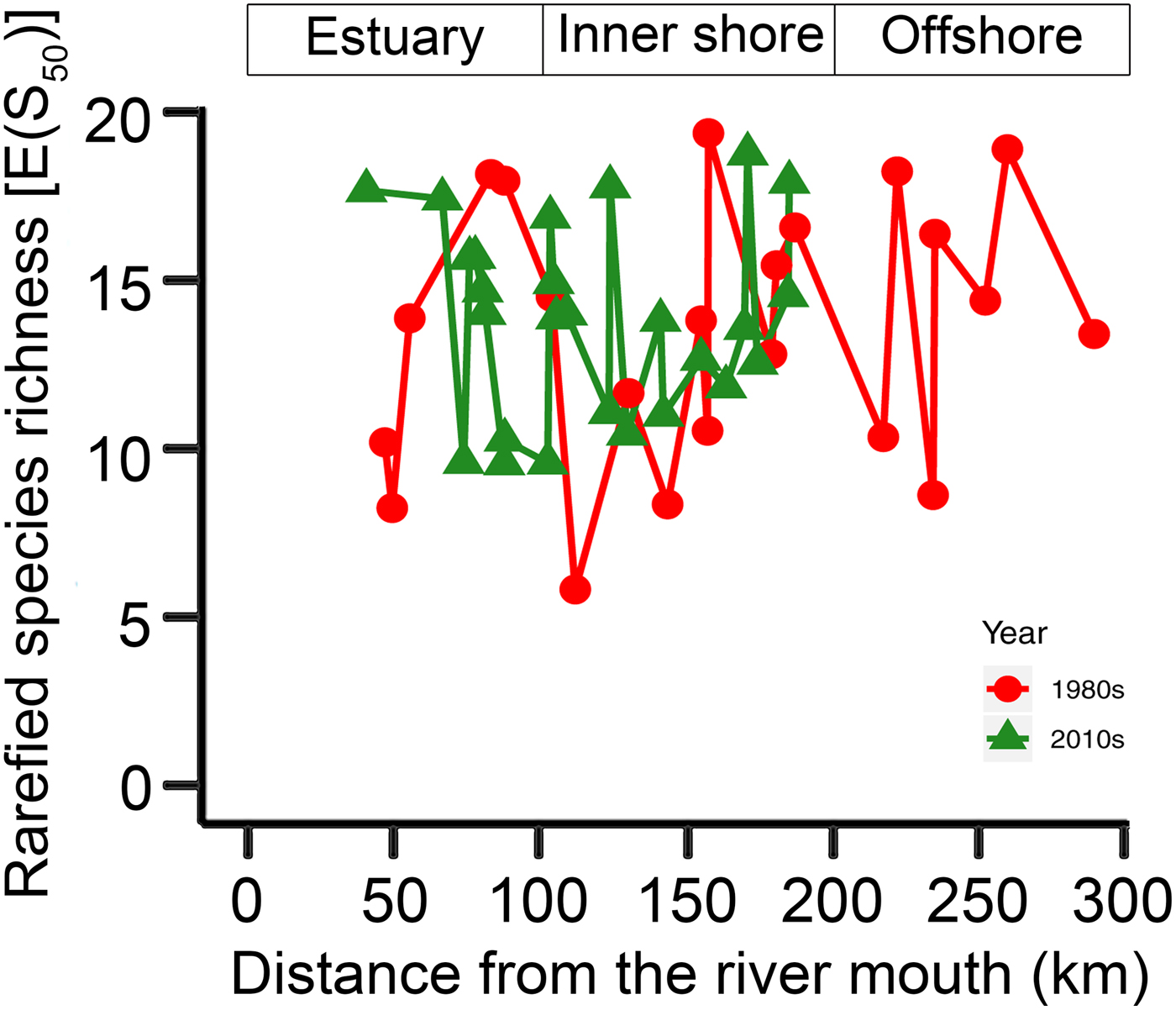
Figure 3. Comparison of rarefied species richness [E(S50)] of ostracode community in the Changjiang estuary and the adjacent East China Sea in the 1980s (gray dashed line) and the 2010s (black solid line). Sampling sites in the 1980s (Wang and Zhao Reference Wang, Zhao and Wang1985; Wang et al. Reference Wang, Zhang, Zhao, Min, Bian, Zheng, Cheng and Chen1988) and the 2010s (this study) are denoted by dots and triangles, respectively. The x-axis is the distance from the river mouth (“X” in Fig. 1; see “Materials and Methods” section).
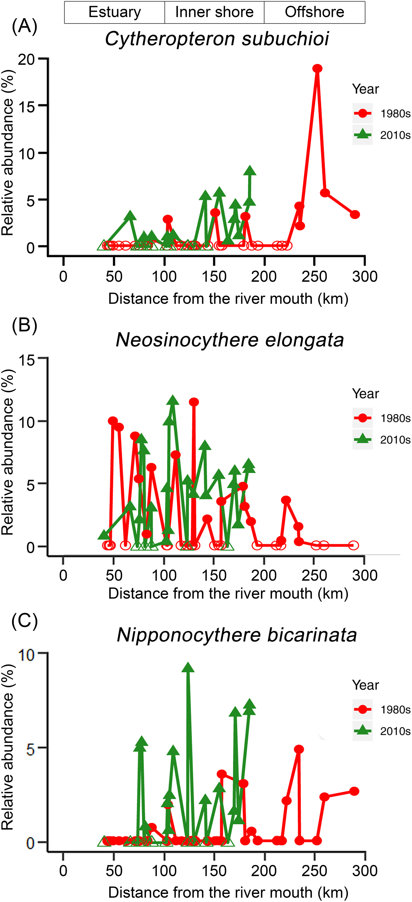
Figure 4. Comparison of percent (relative) abundance of ostracode species. A, Cytheropteron subuchioi; B, Neosinocythere elongata; and C, Nipponocythere bicarinata, in the Changjiang estuary and the adjacent East China Sea in the 1980s (circles) vs. the 2010s (triangles). For sampling sites containing less than 1% of the corresponding species in Wang and Zhao (Reference Wang, Zhao and Wang1985) and Wang et al. (Reference Wang, Zhang, Zhao, Min, Bian, Zheng, Cheng and Chen1988), percent abundance of that corresponding species was truncated to 0.1%. Zero abundance is represented by open circles/triangles. The x-axis is the distance from the river mouth (“X” in Fig. 1; see “Materials and Methods” section).
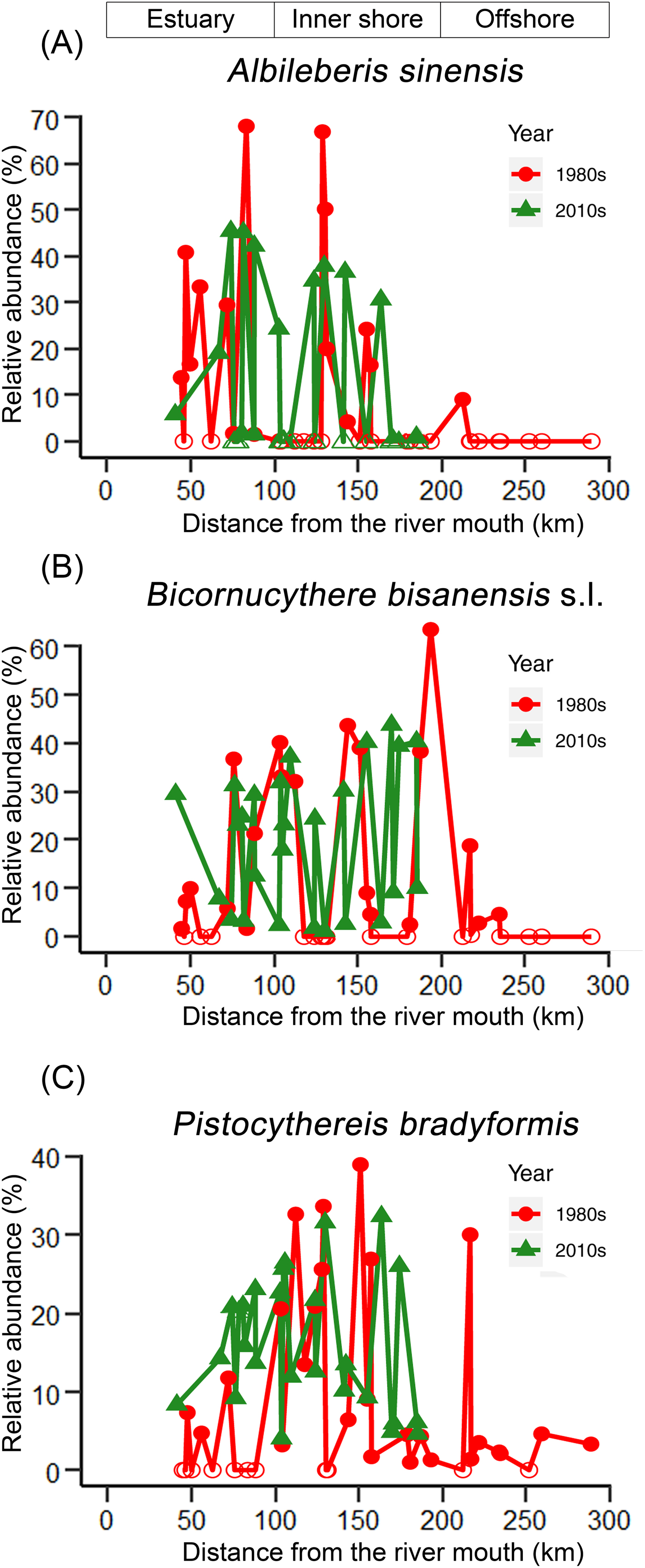
Figure 5. Comparison of percent (relative) abundance of three most abundant ostracode species. A, Albileberis sinensis; B, Bicornucythere bisanensis sensu lato; and C, Pistocythereis bradyformis in the Changjiang estuary and the adjacent East China Sea in the 1980s (circles) vs. the 2010s (triangles). For sampling sites containing less than 1% of the corresponding species in Wang and Zhao (Reference Wang, Zhao and Wang1985) and Wang et al. (Reference Wang, Zhang, Zhao, Min, Bian, Zheng, Cheng and Chen1988), percent abundance of that corresponding species was truncated to 0.1%. Zero abundance is represented by open circles/triangles. The x-axis is the distance from the river mouth (“X” in Fig. 1; see “Materials and Methods” section).
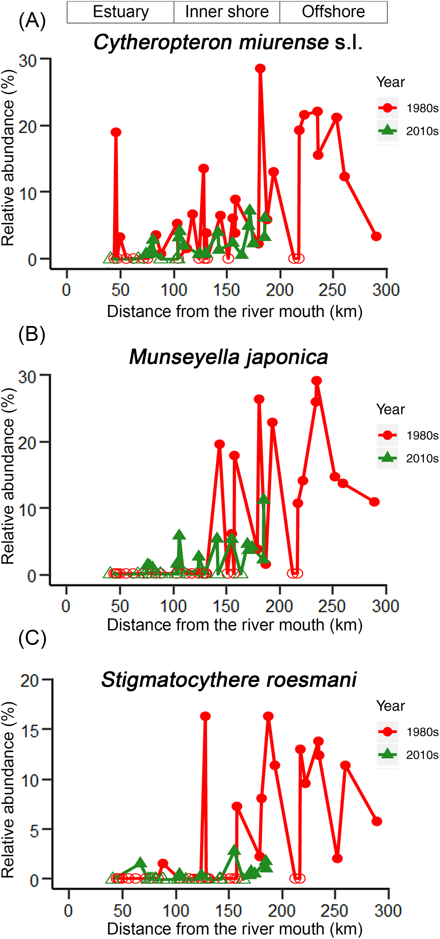
Figure 6. Comparison of percent (relative) abundance of ostracode species. A, Cytheropteron miurense s.l.; B, Munseyella japonica; and C, Stigmatocythere roesmani in the Changjiang estuary and its adjacent East China Sea in the 1980s (circles) vs. the 2010s (triangles). For sampling sites containing less than 1% of the corresponding species in Wang and Zhao (Reference Wang, Zhao and Wang1985) and Wang et al. (Reference Wang, Zhang, Zhao, Min, Bian, Zheng, Cheng and Chen1988), percent abundance of that corresponding species was truncated to 0.1%. Zero abundance is represented by open circles/triangles. Zero abundance is represented by open circles/triangles. The x-axis is the distance from the river mouth (“X” in Fig. 1; see “Materials and Methods” section).
Table 2. Taxonomic synonyms for ostracode species in this study and the studies from the 1980s.

Effects of environmental variables on species composition of 60 ostracode species were tested in RDA. Forward selection of environmental variables retained four significant factors (p < 0.05) for further analysis, namely, bottom-water salinity in January–March and July–September, bottom-water temperature in July–September, and surface productivity in October–December. They jointly accounted for 44.3% (adjusted R 2; p = 0.001) of the variation in the species composition (Table 3). July–September temperature (adjusted R 2 = 0.159; p < 0.001) and salinity (adjusted R 2 = 0.141; p = 0.001) together represent ~68% of the explained variance.
Table 3. Results of the redundancy analysis (RDA) variation partitioning of ostracode community. Spe-Env RDA, environmental predictors in the redundancy analysis model;Spe-Spa RDA, spatial predictors in the redundancy analysis model; MEM, Moran's eigenvector maps; fraction [a] represents pure environmental processes; fraction [c] represents pure spatial processes; fraction [b] represents the shared effect of the two processes; an asterisk (*) indicates significance of the shared fraction is not testable.
Forward selection on the spatial variables resulted in four significant spatial predictors (MEM1, MEM 2, MEM 4, and MEM 7; Supplementary Fig. S7). The spatial model significantly accounted for 41.1% (adjusted R 2; p = 0.001) of the variation of ostracode composition (Table 3).
An RDA plot (Fig. 7, Table 4) showed that Bicornucythere bisanensis (forma P of Abe Reference Abe1988) was negatively related to July–September bottom-water salinity. Its unique position in the lower right quadrant indicated a distinct ecological niche for this species compared with other species in this study. Cytheropteron subuchioi, Cytheropteron miurense sensu lato, Munseyella japonica, Cytherelloidea yingliensis sensu lato, and Bicornucythere bisanensis (forma G of Abe Reference Abe1988) showed a positive relationship with the July–September salinity. Albileberis sinensis was more positively associated with higher July–September bottom-water temperature and lower bottom-water salinity, whereas Nipponocythere bicarinata, Neosinocythere elongata, and Bicornucythere bisanensis (forma G of Abe 1988) were associated with lower July–September bottom-water temperature. Distributions of Trachyleberis niitsumai sensu lato, Keijella apta, Hanaiborchella miurensis, and Cytheromorpha acupunctata were more dependent on lower January–March bottom-water salinity.

Figure 7. Environmental predictors in the redundancy analysis model (Spe-Env RDA) biplots for ostracode compositions. Significant environmental variables are shown. Projecting species objects at right angles on an environmental variable approximates their positions along that variable. Cosine of an angle between response and explanatory variables represents their correlation. janmarSal, bottom-water salinity in January–March period; julyseptSal, bottom-water salinity in July–September; julyseptTemp, bottom-water temperature in July–September; octdecSurfprod, surface productivity in October–December. For species abbreviations, see Table 2.
Table 4. Ostracode species and their codes used in redundancy analysis models.
The whole model of variation partition analysis accounted for 47.3% of the variation of ostracode composition (Fig. 8). The largest explained fraction was attributed to the joint effect of environmental processes and spatial processes fraction [b] (adjusted R 2 = 0.38). A significant pure environmental fraction [a] (adjusted R 2 = 0.063; p = 0.001) and an insignificant pure spatial fraction [c] (adjusted R 2 = 0.03; p = 0.103) were identified (Table 1).

Figure 8. Venn diagram showing results of variation partitioning: [a] is pure environmental fractions, [b] is joint fractions shared by environmental and spatial processes, and [c] is pure spatial fractions. Adjusted R 2 values are reported.
Discussion
Comparing Similarities of Ostracode Compositions in the 1980s and the 2010s
The high sedimentation rate in the study area suggests that ostracode valves collected in this study likely represent the fauna of the 2010s and considerable mixing with older (e.g., 1980s) ostracode valves is unlikely. Moreover, dominant species in our study such as Pistocythereis bradyformis, Bicornucythere bisanensis, Nipponocythere bicarinata, and Sinocytheridea impressa were abundantly found in muddy sediments (Fujiwara et al. Reference Fujiwara, Masuda, Sakai, Irizuki and Fuse2000; Irizuki et al. Reference Irizuki, Takata and Ishida2006; Hong et al. Reference Hong, Yasuhara, Iwatani and Mamo2019). High abundance of these species in our samples indicates a low-energy environment and autochthonous fauna at the sites studied. Clustering results and the NMDS ordination broadly divide ostracode communities into three major groups corresponding to their distances from the coast (Fig. 2). For example, the ES biofacies is comprised of the ostracode assemblage of inner Hanzhou Bay from the 1980s (Fig. 2B) and the coastal assemblage from the 2010s (Fig. 2C). These two assemblages share the same dominant species (i.e., Albileberis sinensis; Fig. 5A). The IS biofacies appears to be found along 123°E in both the 1980s and the 2010s. This is likely due to the dominance of Bicornucythere bisanensis (Fig. 5B) and Pistocythereis bradyformis (Fig. 5C) over the past decades. On the other hand, the OS biofacies, which is dominated by Cytheropteron miurense sensu lato (Fig. 6A), Stigmatocythere roesmani (Fig. 6B), and Munseyella japonica (Fig. 6C) does not have a counterpart in the 2010s.
Impacts of Dams and Anthropogenic Inputs on Ostracode Distribution over the Past 30 Years
Ostracode species such as Cytheropteron subuchioi (Fig. 4A), Neosinocythere elongata (Fig. 4B), and Nipponocythere bicarinata (Fig. 4C) that are known to inhabit relatively offshore, oceanic areas in the China seas and Japanese bays (Zhao and Wang Reference Zhao and Wang1988; Yasuhara et al. Reference Yasuhara, Yoshikawa and Nanayama2005; Yasuhara and Seto Reference Yasuhara and Seto2006; Chunlian et al. Reference Chunlian, Fürsich, Jie, Yixin, Tingting, Jian, Yuan and Min2013) show more landward distribution in the 2010s. The RDA results indicate that these species are more related to saline summer bottom water (Fig. 7). Given that more shoreward intrusion of saline water into the inner-shore area of the Changjiang discharge area has been reported as a consequence of lower summer water discharge of the Changjiang after construction of the TGD (Gong et al. Reference Gong, Chang, Chiang, Hsiung, Hung, Duan and Codispoti2006; Jiao et al. Reference Jiao, Zhang, Zeng, Gardner, Mishonov, Richardson, Hong, Pan, Yan, Jo, Chen, Wang, Chen, Hong, Bai, Chen, Huang, Deng, Shi and Yang2007; Chen et al. Reference Chen, Shiah, Chiang, Gong and Kemp2009; Tsai et al. Reference Tsai, Gong, Sanders, Wang and Chiang2010), the distributional changes of these species likely represent a response to this dam-induced reduction of river water discharge.
Relative abundance of species such as Albileberis sinensis (Fig. 5A), Bicornucythere bisanensis (Fig. 5B), and Pistocythereis bradyformis (Fig. 5C) also increased in the Changjiang discharge area from the 1980s to the 2010s. However, the RDA plot indicates that the driving factors for the distributional changes of these species could be complicated. For example, occurrences of Albileberis sinensis and Cytheromorpha acupunctata are more related to warmer July–September water temperature and higher October–December surface productivity, respectively (Fig. 7), suggesting the potential contribution of hydrological parameters in various seasons. Apart from this, the higher percent abundance of Bicornucythere bisanensis, which is a well-known eutrophication-resistant species (Yasuhara et al. Reference Yasuhara, Yamazaki, Tsujimoto and Hirose2007, Reference Yasuhara, Hunt, Breitburg, Tsujimoto and Katsuki2012a; Irizuki et al. Reference Irizuki, Takimoto, Sako, Nomura, Kakuno, Wanishi and Kawano2011) showing strong positive correlation with total organic carbon content in Kasado Bay, Japan (Irizuki et al. Reference Irizuki, Ito, Sako, Yoshioka, Kawano, Nomura and Tanaka2015), may be attributed to increased organic matter as a result of escalated fertilizer use and sewage discharge in the Changjiang Basin since the 1990s (Chai et al. Reference Chai, Yu, Shen, Song, Cao and Yao2009).
Controlling Factors of Ostracode Species Compositions
Among the environmental factors included in this study (measured during 2005 to 2012), bottom-water temperature and salinity in July–September most significantly explain variation of ostracode composition. Shallow-marine ostracode faunal characteristics and distributions have been related to bottom temperature and/or salinity (Bodergat and Ikeya Reference Bodergat and Ikeya1988; Ozawa et al. Reference Ozawa, Kamiya, Itoh and Tsukawaki2004; Yasuhara et al. Reference Yasuhara, Hunt, van Dijken, Arrigo, Cronin and Wollenburg2012b), in particular, some species may respond to seasonal variation of environmental variables (Brouwers et al. Reference Brouwers, Cronin, Horne and Lord2000). The greater importance of environmental variables in July–September may be related to ostracode species tolerance limits with respect to the summer environment, that is, maximum temperature and/or minimum salinity, which can potentially be regulated by variability of the TWC strength (a branch of Kuroshio Current), climate variables (e.g., monsoon precipitation), and water discharge patterns of the Changjiang.
A large proportion of the variation in ostracode composition is explained by the fraction of spatially structured environmental variables (fraction [b]; Fig. 8). This fraction could either be attributed to spatially structured environmental variables (i.e., bottom-water temperature and salinity) or to spatial variation of some unobserved environmental factors that affected both the ostracode community structure and the explanatory variables in the analysis (Legendre and Legendre Reference Legendre and Legendre2012). Adjusted R 2 values of the purely environmental component [a] and purely spatial component [c] are relatively low, yet they are consistent with the results of De Bie et al. (Reference De Bie, De Meester, Brendonck, Martens, Goddeeris, Ercken, Hampel, Denys, Vanhecke, Van der Gucht, Van Wichelen, Vyverman and Declerck2012), who reported the explained variation by other passively dispersed aquatic organisms driven by [a] and [c].
Dispersal is an important mechanism in community structure assembly. A limited dispersal rate prohibits species reaching their preferred habitats, while a high dispersal rate leads to overdispersal such that species occur in unfavorable environments (Heino et al. Reference Heino, Melo, Siqueira, Soininen, Valanko and Bini2015). Both of these scenarios can result in significant spatial signals. On the other hand, a significant environmental signal (i.e., species-sorting mechanism) indicates that species get sorted to their favorable habitats (Leibold et al. Reference Leibold, Holyoak, Mouquet, Amarasekare, Chase, Hoopes, Holt, Shurin, Law and Tilman2004). The variation partitioning results show that environmental processes are significant but spatial processes are insignificant, suggesting that ostracode species composition is structured by species sorting coupled with a moderate dispersal rate (Ng et al. Reference Ng, Carr and Cottenie2009). Shallow-marine ostracodes are generally poor dispersers that migrate by either “walking” or being carried by vectors such as ocean currents, ballast water, and flowing weed (Teeter Reference Teeter1973; Titterton and Whatley Reference Titterton and Whatley1988). Passive migration due to fast-flowing (~26–34 cm/s) bottom-water current has been proposed as a controlling factor in recent distribution of warm, shallow-marine ostracode species in Japan (Tanaka Reference Tanaka2008). The subsurface TWC, which can reach a maximum flow rate of ~30 cm/s (Zhu et al. Reference Zhu, Chen, Ding, Li and Lin2004) may, therefore, potentially aid dispersal of ostracode species to favorable environments, while the rapid generation of shallow-marine ostracodes (Smith and Horne Reference Smith, Horne, Holmes and Chivas2012) promotes their colonization.
Conclusions
Our results describe biotic responses to rapid environmental changes in the Changjiang delta. While ostracode species richness in the study area does not show systematic change relative to that of the 1980s, changes in relative abundance of key species showed characteristic patterns. These possibly resulted from anthropogenic activities such as urban development (i.e., eutrophication) and construction of dams (i.e., reduction of river water discharge). We have also demonstrated that environmental processes are more important than spatial processes for ostracode community structure in Changjiang estuary and its adjacent area. Integrating spatial variables generated by methods such as dbMEM into analysis not only improves our understanding of the mechanisms leading to the observed species distribution pattern, but also provokes consideration of context-dependent false-positive species–environment correlations represented by the explained variation of spatially structured environmental variables. Although this approach was recently applied on freshwater ostracode analyses (Escrivà et al. Reference Escrivà, Poquet and Mesquita-Joanes2015; Zhai et al. Reference Zhai, Nováček, Výravský, Syrovátka, Bojková and Helešic2015; Castillo-Escrivà et al. Reference Castillo-Escrivà, Valls, Rochera, Camacho and Mesquita-Joanes2016), it has been underappreciated in marine ostracode studies. This study assesses ecological impacts of deteriorating Asian mega-deltas and is especially significant for paleontological studies that derive past environmental conditions based on knowledge of modern species–environmental relationships.
Acknowledgments
We thank the editors and reviewers for their constructive comments; Q. Zhao for providing Chinese ostracode data from the 1980s; P. Wong for processing GIS environmental data; and L. Wong, M. Lo, and the staff of the Electronic Microscope Unit of the University of Hong Kong for their continuous support. The work described in this paper was partially supported by the Earth as a Habitable Planet Thesis Development Grant of the University of Hong Kong (to R.C.W.C.), the General Research Fund of the Research Grants Council of Hong Kong (project code: HKU 17303115), the Early Career Scheme of the Research Grants Council of Hong Kong (project code: HKU 709413P), the Seed Funding Programme for Basic Research of the University of Hong Kong (project codes: 201111159140 and 201611159053) (to M.Y.), and the National Basic Research Program of China (2013CB956504) (to Y.-w.D.).