


Introduction
Oceanic anoxic events (OAEs) occur when the oxygen minimum zone (OMZ)—a normal component of open-marine systems—expands, causing shallow continental shelf habitats to experience significant depletion in dissolved oxygen from the thermocline into the photic zone (Schlanger and Jenkyns Reference Schlanger and Jenkyns1976; Kuypers et al. Reference Kuypers, Lourens, Rijpstra, Pancost, Nijenhuis and Sinninghe Damsté2004). OMZs form at several hundred meters depth where the balance between oxygen supply and organic decay results in low oxygen concentrations (Schlanger and Jenkyns Reference Schlanger and Jenkyns1976; Lalli and Parsons Reference Lalli and Parsons1993). Today, OMZs may have oxygen concentrations as low as 10% of normal ocean conditions (Lalli and Parsons Reference Lalli and Parsons1993). OMZ expansion can result from increased input of detrital organic matter (e.g., resulting from increased planktonic productivity) into the ocean system (Schlanger and Jenkyns Reference Schlanger and Jenkyns1976; Skelton et al. Reference Skelton, Spicer, Kelley and Gilmour2006) and/or increased temperature, because warm water holds less dissolved oxygen (Falkowski et al. Reference Falkowski, Algeo, Codispoti, Deutsch, Emerson, Hales and Huey2011).
Phanerozoic deoxygenation events brought on by OMZ expansion have been linked to external factors such as increased weathering, sediment, and nutrient flux to the ocean (Monteiro et al. Reference Monteiro, Pancost, Ridgwell and Donnadieu2012; Pogge von Strandmann et al. Reference Pogge von Strandmann, Jenkyns and Woodfine2013; Owens et al. Reference Owens, Lyons and Lowery2018). This is often attributed to increased seafloor spreading rates and the emplacement of Large Igneous Provinces (LIPs), both of which may cause increased CO2 flux to the atmosphere and increased temperature (Leckie et al. Reference Leckie, Bralower and Cashman2002; Snow et al., Reference Snow, Duncan and Bralower2005; Sageman et al. Reference Sageman, Meyers and Arthur2006; Jenkyns Reference Jenkyns2010; Barclay et al. Reference Barclay, McElwain and Sageman2010; van Bentum et al. Reference van Bentum, Reichart, Forster and Sinninghe Damsté2012; Pogge von Strandmann et al. Reference Pogge von Strandmann, Jenkyns and Woodfine2013; Owens et al. Reference Owens, Lyons and Lowery2018). As a result, large swaths of the world's shallow oceans become severely oxygen depleted (Schlanger and Jenkyns Reference Schlanger and Jenkyns1976). In the geologic record, OAEs are identified by a net sequestration of carbon, which may be observed as packages of organic-rich, laminated black shale deposits and abrupt δ13C excursions (CIEs; up to ±5‰ depending on the source of CO2; Erbacher et al. Reference Erbacher, Thurow and Lattke1996; Sageman et al. Reference Sageman, Meyers and Arthur2006; Owens et al. Reference Owens, Lyons and Lowery2018).
Due to their global extent and severity, OAEs have the potential to cause significant extinction, particularly in shallow coastal systems. For example, OAEs have been associated with higher rates of biotic turnover during the Permo-Triassic and Triassic–Jurassic mass extinctions (Wignall and Twitchett Reference Wignall and Twitchett1996; Kiessling et al. Reference Kiessling, Aberhan, Brenneis and Wagner2007; Kiessling and Aberhan Reference Kiessling and Aberhan2007a,Reference Kiessling and Aberhanb). More specifically, significant foraminiferal turnover was observed coeval with several Cretaceous OAEs (Erba Reference Erba1994; Leckie et al, Reference Leckie, Bralower and Cashman2002; Parente et al. Reference Parente, Frijia, Di Lucia, Jenkyns, Woodfine and Baroncini2008), and reef declines have also been connected with OAE activity (Arthur and Schlanger Reference Arthur and Schlanger1979; Gröstsch et al. Reference Grötsch, Schroeder, Noé and Flügel1993; Föllmi et al. Reference Föllmi, Weissert, Bisping and Funk1994; Weissert et al. Reference Weissert, Lini, Föllmi and Kuhn1998; Phelps et al. Reference Phelps, Kerans, Da-Gama, Jeremiah, Hull and Loucks2015).
However, there is also evidence that some OAEs are not associated with extinctions, or have only impacted select taxa; for example, the Toarcian OAE (~183 Ma) likely had little to no effect on belemnites (Ullmann et al. Reference Ullmann, Thibault, Ruhl, Hesselbo and Korte2014). Beyond the effect of OAEs on raw diversity and extinction rates, there is additional uncertainty surrounding their ecological selectivity, especially regarding whether selectivity patterns were unique from background selection regimes (e.g., the differences between Kiessling et al. [Reference Kiessling, Aberhan, Brenneis and Wagner2007] and Clapham and Payne [Reference Clapham and Payne2011]). These discrepancies indicate that the precise influence of OAEs on marine fauna is not well known.
Mollusks are an important clade for testing the impact of OAEs; they are the most diverse invertebrate phylum (23% of all marine species; Sepkoski Reference Sepkoski1981; Appeltans et al. Reference Appeltans, Ahyong, Anderson, Angel, Artois, Bailly and Bamber2012) and the largest phylum represented in the fossil record, because they demonstrate relatively high and comparatively uniform preservation potential (Kidwell Reference Kidwell2002, Reference Kidwell2005). Thus, restricting analyses to mollusks minimizes biases surrounding rarity and taphonomy, while preserving sufficient sample sizes to facilitate statistical analyses. Moreover, of all marine invertebrate clades, mollusks are the second-most tolerant to low-oxygen conditions, superseded only by foraminifera (Baker and Mann Reference Baker and Mann1992; Moodley and Hess Reference Moodley and Hess1992; Ekau et al. Reference Ekau, Auel, Pörtner and Gilbert2010; Song et al. Reference Song, Wignall, Chu, Tong, Sun, Song, He and Tan2014).
The Cretaceous marine fossil record is particularly well sampled globally (Erbacher et al. Reference Erbacher, Thurow and Lattke1996; Kuypers et al. Reference Kuypers, Lourens, Rijpstra, Pancost, Nijenhuis and Sinninghe Damsté2004; Sageman et al. Reference Sageman, Meyers and Arthur2006; Forster et al. Reference Forster, Kuypers, Turgeon, Brumsack, Petrizzo and Sinninghe Damsté2008; Elrick et al. Reference Elrick, Moline-Garza, Duncan and Snow2009; Li et al. Reference Li, Montañez, Liu and Ma2017), and consequently provides an ideal opportunity to test the influence of widespread anoxia on molluscan biodiversity, extinction, and ecological structure. There were as many as six OAEs during the Cretaceous Period: OAE1a (early Aptian; lasting ~1.0–1.3 Myr), OAE1b (Aptian/Albian; ~4.0 Myr), OAE1c (late Albian; <0.2 Myr), OAE1d (Albian/Cenomanian; ~0.5 Myr), OAE2 (Cenomanian/Turonian; ~0.82 Myr), and OAE3 (late Coniacian; ~1.1 Myr) (Schlanger and Jenkyns Reference Schlanger and Jenkyns1976; Leckie et al. Reference Leckie, Bralower and Cashman2002; Gröcke et al. Reference Gröcke, Ludvigson, Witzke, Robinson, Joeckel, Ufnar and Ravn2006; Y. Li et al. Reference Li, Bralower, Montañez, Osleger, Arthur, Bice, Herbert, Erba and Silva2008; Millán et al. Reference Millán, Weissert and Lópes-Horgue2014; Joo and Sageman Reference Joo and Sageman2014; X. Li et al. Reference Li, Montañez, Liu and Ma2017). Of these, OAE1b and OAE2 were the most severe and/or widespread, each presenting a >2‰ positive CIE and extensive black shale deposition (Leckie et al. Reference Leckie, Bralower and Cashman2002; Monteiro et al. Reference Monteiro, Pancost, Ridgwell and Donnadieu2012; Joo and Sageman Reference Joo and Sageman2014). OAE3 shows the smallest CIE and is potentially a regional rather than a global event (Wagreich Reference Wagreich2012; Lowery et al. Reference Lowery, Leckie and Sageman2017).
These OAEs occurred within the larger Cretaceous greenhouse climate system; gradual warming began at the Hauterivian/Barremian boundary (Frakes Reference Frakes1999; Fig. 1C) and continued until the middle Turonian (Clarke and Jenkyns Reference Clarke and Jenkyns1999; Li and Keller Reference Li and Keller1999; Friedrich et al. Reference Friedrich, Norris and Erbacher2012; Jarvis et al. Reference Jarvis, Lignum, Gröcke, Jenkyns and Pearce2011). Subsequent gradual cooling continued into the Paleocene, but included numerous relatively rapid warming/cooling events throughout (Clarke and Jenkyns Reference Clarke and Jenkyns1999; Li and Keller Reference Li and Keller1999; Jarvis et al. Reference Jarvis, Lignum, Gröcke, Jenkyns and Pearce2011; Friedrich et al. Reference Friedrich, Norris and Erbacher2012; O'Brien et al. Reference O'Brien, Robinson, Pancost, Sinninghe Damsté, Schouten, Lunt and Alsenz2017).
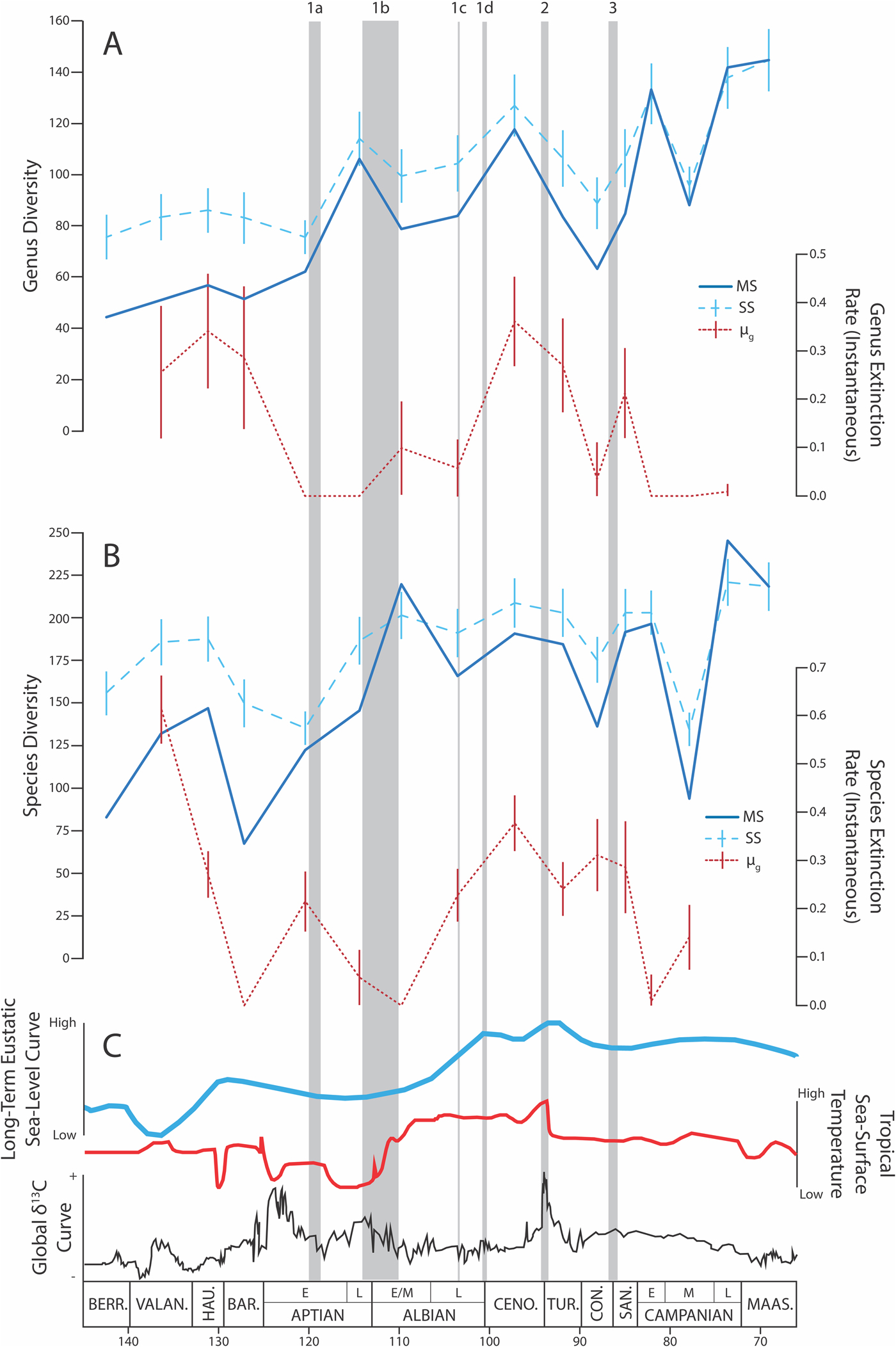
Figure 1. Timeline of diversity (including multiton subsampling [MS; Alroy Reference Alroy2017b] and sample-standardized [SS; for examples, see Bush et al. Reference Bush, Markey and Marshall2004; Kiessling et al. Reference Kiessling, Aberhan, Brenneis and Wagner2007] diversity estimates), instantaneous extinction rate (μg; Alroy Reference Alroy2014), and environmental factors during the Cretaceous Period. Error bars on SS diversity show 2 SDs. OAEs are named and denoted with shaded gray bars according to their specific timing and duration. A, Genus-level diversity (MS and SS) and extinction rate (μg) patterns. B, Species-level diversity (MS and SS) and extinction rate (μg) patterns. C, Long-term eustatic sea-level curve (modified from Ogg et al. Reference Ogg, Ogg and Gradstein2016), long-term tropical sea-surface temperature curve, and global δ13C curve (both modified from the TimeScale Creator [Ogg et al. Reference Ogg, Ogg and Gradstein2016]). BERR., Berriasian; VALAN., Valanginian; HAU., Hauterivian; BAR., Barremian; CENO., Cenomanian; TUR., Turonian; CON., Coniacian; SAN., Santonian; MAAS., Maastrichtian.
OAE2 (aka the Bonarelli event) is considered by far the most severe Cretaceous OAE (Erbacher et al. Reference Erbacher, Thurow and Lattke1996; Kuypers et al. Reference Kuypers, Lourens, Rijpstra, Pancost, Nijenhuis and Sinninghe Damsté2004; Sageman et al. Reference Sageman, Meyers and Arthur2006; Forster et al. Reference Forster, Kuypers, Turgeon, Brumsack, Petrizzo and Sinninghe Damsté2008; Elrick et al. Reference Elrick, Moline-Garza, Duncan and Snow2009; Baroni et al. Reference Baroni, Topper, van Helmond, Brinkhius and Slomp2014; Joo and Sageman Reference Joo and Sageman2014; Li et al. Reference Li, Montañez, Liu and Ma2017; Owens et al. Reference Owens, Lyons and Lowery2018). The abrupt CIE observed at this time ranges from + 2.5 to 7‰, and averages around + 3‰ globally (Owens et al. Reference Owens, Lyons and Lowery2018). While the rate of seafloor spreading was high at this time, the massive amount of warming and CO2 flux is more likely associated emplacement of the Caribbean LIP, which is thought to have triggered the onset of rapid warming (Erba Reference Erba1994; Leckie et al. Reference Leckie, Bralower and Cashman2002; Parente et al. Reference Parente, Frijia, Di Lucia, Jenkyns, Woodfine and Baroncini2008; Turgeon and Creaser Reference Turgeon and Creaser2008; Elrick et al. Reference Elrick, Moline-Garza, Duncan and Snow2009; Barclay et al. Reference Barclay, McElwain and Sageman2010; although see Jarvis et al. [2011] for evidence of brief cooling—the Plenus cold event—just before the most severe anoxia).
Paleobiologically, OAE2 is coincident with the 10th largest extinction event during the Phanerozoic (Raup and Sepkoski Reference Raup and Sepkoski1984; Bambach et al. Reference Bambach, Knoll and Wang2004; Bambach Reference Bambach2006). Approximately 25% of all marine genera and 33–53% of all marine species went extinct; this represents ~2.5 times the average background-extinction percentage for genera at the time (Bambach Reference Bambach2006). Several studies have shown that microfauna such as foraminifera show considerable turnover across OAE2 (e.g., Erba Reference Erba1994; Leckie et al. Reference Leckie, Bralower and Cashman2002; Parente et al. Reference Parente, Frijia, Di Lucia, Jenkyns, Woodfine and Baroncini2008).
This investigation tests the influence of OAE2 on molluscan biodiversity, extinction, and ecological structure using a quantitative occurrence–based approach made possible by the Paleobiology Database (PBDB; http://www.paleobiodb.org). Previous studies of molluscan diversity at this time provide contradictory results. Some have shown that only a regional loss of ammonite species diversity occurred across OAE2 and that the loss was primarily due to a decrease in origination rates (e.g., Monnet and Bucher Reference Monnet and Bucher2007; Monnet Reference Monnet2009). Others suggest upward of a 60% decrease in global ammonite generic diversity (Elder Reference Elder1989; Harries and Little Reference Harries and Little1999; Hirano et al. Reference Hirano, Toshimitsu, Matsumoto, Takahashi, Okada and Mateer2000; Bambach Reference Bambach2006; Jagt-Yazykova Reference Jagt-Yazykova2011, Reference Jagt-Yazykova2012). There is also debate regarding the timing of molluscan turnover, that is, whether extinctions were directly tied to OAE2 (Harries and Little Reference Harries and Little1999; Bambach Reference Bambach2006) or whether the extinction largely predated the Bonarelli event (Fisher Reference Fisher2006; Monnet and Bucher Reference Monnet and Bucher2007; Monnet Reference Monnet2009; Kaiho et al. Reference Kaiho, Katabuchi, Oba and Lamolda2014). Notably, many of these studies compared data gathered from select sites at the local/regional scale; whereas the analyses described here estimate diversity and extinction patterns at the global scale with stage-level temporal resolution (comparable to other diversity studies at different time intervals; e.g., Sepkoski Reference Sepkoski1981; Raup and Sepkoski Reference Raup and Sepkoski1982, Reference Raup and Sepkoski1984, Reference Raup and Sepkoski1986; Jablonski Reference Jablonski1986; Foote Reference Foote2000; Alroy et al. Reference Alroy, Marshall, Bambach, Bezusko, Foote, Fürsich and Hansen2001; Bush et al. Reference Bush, Markey and Marshall2004; Kiessling and Aberhan Reference Kiessling and Aberhan2007a,Reference Kiessling and Aberhanb; Kiessling et al. Reference Kiessling, Aberhan, Brenneis and Wagner2007; Alroy Reference Alroy2008, Reference Alroy, Alroy and Hunt2010a; Clapham and Payne Reference Clapham and Payne2011).
Methods
All analyses for this study were performed in R (v. 3.2.4; R Core Development Team 2017). MS code was provided by Alroy (Reference Alroy2017a).
Taxonomic Sampling
Global occurrence data for marine molluscan taxa were downloaded from the PBDB on 6 August 2018. These data spanned the Tithonian (latest Jurassic) through the Danian (earliest Paleogene) stages. The data were filtered to include: only genera whose taxonomy was included in Sepkoski's (Reference Sepkoski2002) compendium, as it is considered to be the most comprehensive and most broadly accepted consensus of fossil marine animal genera; taxa that were identified to the species level (for species–genera comparisons); and individual occurrences that could be stratigraphically constrained to the geologic stage level (~5 Myr each). Binning occurrence data at this temporal resolution (4–6 Myr) has previously been shown to reveal meaningful changes in both ecology and diversity (Kiessling et al. Reference Kiessling, Aberhan, Brenneis and Wagner2007; Kiessling and Aberhan Reference Kiessling and Aberhan2007a,Reference Kiessling and Aberhanb; Clapham and Payne Reference Clapham and Payne2011; Supplementary Table S1).
Because some Cretaceous stages (Aptian, Albian, and Campanian) are approximately twice this duration (~12 Myr), these stages were split into substages (early Aptian, late Aptian, early/middle Albian, late Albian, early Campanian, middle Campanian, and late Campanian) to reduce bias from variable temporal bin sizes. Finer temporal resolution (i.e., substage level) is not consistently reported in the occurrence data available through the PBDB. Thus, the analyses were limited to ~5 Myr temporal bins. This resulted in diversity, extinction, and ecological analysis across 16 Cretaceous time bins (Table 1).
Table 1. Results of the multiton subsampling (MS) and sample-standardized (SS) estimates for all 16 Cretaceous time bins at both the genus and species levels. SS diversities include mean diversity of 999 replicates ± 2 SDs.

Stratigraphic singletons were removed to reduce the uncertainty in distinguishing rare taxa from those subject to taphonomic or sampling biases (Foote Reference Foote1997, Reference Foote2000; Lenat and Resh Reference Lenat and Resh2001). Stratigraphic singletons were defined as taxa that did not have at least one occurrence in any preceding and following geologic stage (e.g., occurred in the Cenomanian, but not in the Albian or Turonian; for additional examples, see Sepkoski Reference Sepkoski1997; Alroy Reference Alroy2000; Alroy et al. Reference Alroy, Marshall, Bambach, Bezusko, Foote, Fürsich and Hansen2001; Kiessling et al. Reference Kiessling, Aberhan, Brenneis and Wagner2007). We used the Tithonian and Danian stages to determine the presence of singletons for the Berriasian and Maastrichtian, respectively; Tithonian and Danian occurrences were not independently analyzed for changes in diversity or ecology. Even data treated in this manner have the potential to contain edge effects; however, the OAE-bounded intervals that we focused on are in the middle of our time series, rendering these edge effects unlikely to influence impacts of OAEs on diversity patterns. The resulting data set included 1029 genera, 11,599 species, and 53,084 molluscan occurrences (see Supplementary Table S1 for raw PBDB data and Supplementary Table S2 for the cleaned data set).
A significant proportion of large-scale paleobiological studies are conducted on genus-level taxonomic data (e.g., Simpson Reference Simpson1961; Allmon Reference Allmon1992; Sepkoski Reference Sepkoski1998). This is in part because species-level identifications are often considered less robust than those binned within genera (Raup and Sepkoski Reference Raup and Sepkoski1982; Wheeler and Meier Reference Wheeler and Meier2000). However, given the potential for higher-level taxonomy to dilute or even obscure species-level patterns (Hendricks et al. Reference Hendricks, Saupe, Myers, Hermsen and Allmon2014), we evaluated the difference between generic and species data sets explicitly by performing analyses at both taxonomic levels. This resulted in 32 data sets for diversity and ecological analysis: 16 time bins for each of two taxonomic levels.
Taxonomic Diversity
Taxonomic diversity was calculated using multiton subsampling (MS) on all 32 data sets (Alroy Reference Alroy2017a,Reference Alroyb). In comparison studies, MS has been shown to be a more robust method of estimating diversity than previous methods of fair/coverage-based sampling (e.g., shareholder quorum subsampling or extrapolation methods; Alroy Reference Alroy, Alroy and Hunt2010a,Reference Alroyb, Reference Alroy2017a,Reference Alroyb). MS also performs better than more traditional methods of sample-standardized (SS) diversity estimates, because it avoids issues such as flattening of diversity curves (Alroy Reference Alroy, Alroy and Hunt2010a,Reference Alroyb, Reference Alroy2017b), although we also estimated diversity using the SS method for comparison. We calculated diversity using both MS and SS methods for all Cretaceous time bins at both the genus and species levels (see the Methods Appendix in the Supplementary Material for a more detailed explanation).
Extinction Rates
Extinction rates were calculated on the genus- and species-level data sets using two different techniques: the Alroy (Reference Alroy2008) three-timer rate (μ3) and the Alroy (Reference Alroy2014) gap-filler rate (μG). To calculate confidence intervals on our extinction rates, we rarefied both our genus- and species-level data sets 999 times, selecting one-third of each data set with replacement in every repetition, and then calculated the μ3 and μG extinction rates (see the Methods Appendix in the Supplementary Material for a more detailed explanation).
Ecology
To estimate ecological selectivity of diversity patterns across each time bin, we tested the relationship between taxon survivorship and taxon ecology using generalized linear models (GLMs) for single and multiple logistic regression. Logistic regression is ideal for extinction-related studies, as the outcome of selectivity is binary (i.e., the species either went extinct or survived; for additional examples, see Clapham and Payne Reference Clapham and Payne2011; Payne et al. Reference Payne, Bush, Chang, Heim, Knope and Pruss2016a,Reference Payne, Bush, Heim, Knope and McCauleyb). Taxa were classified into broad ecological categories according to clade membership, faunality, mobility, and feeding strategy, based on PBDB descriptions that are broadly determined by prior morphological analysis (Supplementary Table S1). Clade membership was assigned at the class level: Bivalvia, Cephalopoda, and Gastropoda. Scaphopoda and Polyplacophora were represented by a combined three genera for the entire occurrence data set; thus, they were used for diversity and extinction calculations, but not for ecological analysis. Clade membership and feeding strategies were considered categorical variables (ranked either 0 or 1 for each subcategory), whereas faunality and mobility were treated as ordinal variables. Feeding strategies were categorized as: filter feeding, suspension feeding, detritivorous, carnivorous, and grazing. Omnivores and chemosymbionts were present but rare; these taxa were also retained for investigating diversity and extinction patterns but removed for the ecological analyses. Faunality was assigned to each taxon along an increasingly bottom-dwelling to pelagic gradient as either infaunal (1), semi-infaunal (2), epifaunal (3), or nektonic/nektobenthic (4). Mobility was classified as stationary (1), facultatively mobile (2), or actively mobile (3). Survivorship was categorized as extant (1) in the time bin of the taxon's first occurrence until the time bin of last occurrence, even if the taxon did not occur in an intermediate time bin; the taxon was labeled extinct (0) in the time bin of its last occurrence and not present (NA) in all bins before its first occurrence and following its last occurrence. Thus, Lazarus taxa were categorized as extant in time bins where they failed to occur. Because there were no intrageneric differences in assigned ecological traits in the PBDB, we performed this analysis using the generic data sets only.
The majority of ecological classifications from the PBDB are made at the genus or the family level. However, some are made at the class or ordinal level. Across our 32 data sets approximately 10% of genera were assigned ecological classifications at the genus level. Approximately 62% and 28% of taxa were classified at the family/subfamily and class/order levels, respectively. Because this may bias genus-level analyses of ecological selectivity, we performed two sets of sensitivity analyses that tested for ecological selectivity among: (1) only those taxa with ecological classifications at the genus level and (2) only those taxa with ecological classifications at the family level and below. Sensitivity analyses provided results identical to those for the full data sets, and therefore these results are not reported separately.
To better understand the causal relationships between survivorship and combinations of ecological traits, we examined five GLM models testing specific hypotheses of OAE ecological selectivity. These hypotheses were generated a priori based on the current best understanding of molluscan responses to environmental change to avoid introducing biases from data dredging/p-hacking. All models included the impact of molluscan clade membership (i.e., Bivalvia, Cephalopoda, and Gastropoda) on survivorship to test for phylogenetic independence.
The first model represented a “full model” (model 1), which tested the hypothesis that survivorship depended on the interactions of all measured ecological characteristics (clade membership, faunality, mobility, and all feeding categories: detritivores, carnivores, suspension feeders, and grazers). Four subsets of the full model tested hypotheses with existing theoretical or empirical support as drivers of survivorship given the low oxygen conditions associated with OAEs. Faunality was included in all models, as OAEs are characterized by severely reduced oxygen in the shallow shelf environments preferred by mollusks. For example, Clapham and Payne (Reference Clapham and Payne2011) found that infaunal taxa were more likely to go extinct than epifaunal taxa at the end-Permian—when there was severe anoxia—as OMZ expansion onto the shallow shelf should affect the benthos before the rest of the water column (Schlanger and Jenkyns Reference Schlanger and Jenkyns1976; Clapham and Payne Reference Clapham and Payne2011). Thus, model 2 tested the hypothesized effects of clade membership and faunality in controlling survivorship.
Model 3 tested the influence of clade membership, feeding strategy, and faunality on patterns of survivorship. We hypothesized that suspension feeders and detritivores would demonstrate increased survivorship relative to carnivores and grazers across time bins that contained/were bound by an OAE due to the large increase in detrital organic matter resulting from increased anoxia-driven mortality. Aberhan and Baumiller (Reference Aberhan and Baumiller2003) note that after the Triassic–Jurassic mass extinction (which includes the influence of an OAE), the bivalve community was nearly devoid of infaunal suspension feeders. Furthermore, grazers were found to be negatively impacted across the Permo-Triassic mass extinction (Xie et al. Reference Xie, Pancost, Wang, Yang, Wignall, Luo, Jia and Chen2010), potentially due to the emergence of cyanobacteria as the dominant primary producers at the time (Ohkouchi et al. Reference Ohkouchi, Kashiyama, Kuroda, Ogawa and Kitazako2006; Kashiyama et al. Reference Kashiyama, Ogawa, Kuroda, Shiro, Nomoto, Tada and Kitazato2008; Paul Reference Paul and Hudnell2008). We hypothesized carnivores to decrease in diversity due to increased prey mortality resulting from anoxia and because carnivory has been shown to require higher oxygen concentrations for both prey capture and metabolism (Sperling et al. Reference Sperling, Frieder, Raman, Girguis, Levin and Knoll2013).
Model 4 tested for the effects of clade membership, faunality, plus only detritivory and suspension feeding on survivorship. This model represented the combination of the two feeding strategies hypothesized to perform well (suspension feeders and detritivores) relative to the two feeding strategies we hypothesized to show increased extinction (grazers and carnivores). Model 5 tested for the relationship between clade membership, faunality, mobility, detritivory, suspension feeding, and survivorship. The inclusion of mobility tested the prediction that actively mobile taxa may be more likely to access surface waters, which would have had the highest dissolved oxygen content.
The likelihood of the hypotheses associated with each model was estimated using the Akaike information criterion (AIC values) and associated Akaike weights (w i; Akaike Reference Akaike1974); models with more support have lower AIC values and higher w i values. Models within two AIC of each other are similarly well supported by the data (Burnham and Anderson Reference Burnham and Anderson2002), hence all models within two AIC of the model with the lowest AIC should be considered good explanatory candidates. Absolute model explanatory power was assessed by comparison of null and residual deviances (Anderson and Burnham Reference Anderson and Burnham2002; Burnham and Anderson Reference Burnham and Anderson2002).
Results
Diversity Dynamics and Extinction Rates
The pattern of Cretaceous diversity recovered in these analyses is similar across both methodologies for subsampling (MS and SS) and both taxonomic levels (genus and species; Fig. 1). MS recovers significant generic diversity declines across four time bins: the late Aptian/early–middle Albian, Cenomanian/Turonian, Turonian/Coniacian, and early Campanian/middle Campanian boundaries. We primarily interpret MS-derived diversity and gap-filler extinction rates (μG), as these are the preferred methods for unbiased diversity and extinction rate estimation and are not subject to the biases of flattened diversity estimates and “un-fair” methods of sampling (Alroy Reference Alroy, Alroy and Hunt2010a,Reference Alroyb, Reference Alroy2014, Reference Alroy2017b; see Supplementary Table 1 for a direct comparison between μ3 and μG extinction rate estimations).
Figure 1 and Table 1 provide results of molluscan diversity and extinction rate estimates for the entire Cretaceous. The genus-level analysis supports the hypothesis that OAE2 resulted in substantially increased extinction rates and decreases in diversity (Fig. 1A; Leckie et al. Reference Leckie, Bralower and Cashman2002; Kuhnt et al. Reference Kuhnt, Holbourn and Moullade2011; Joo and Sageman Reference Joo and Sageman2014). OAE1b also shows a decreased diversity in the early–middle Albian, but this is not supported by increased extinction rates (Fig. 1A). In addition to significant diversity decreases, three pulses of diversity increase were recovered through the middle part of the Cretaceous: across the early Aptian/late Aptian, the late Albian/Cenomanian, and Coniacian through early Campanian boundaries. These intervals were not associated with decreases in extinction rates.
Ecology
Table 2 provides the results of the GLMs quantitatively testing the relationships between taxon survivorship and specific combinations of ecological traits. Of the five hypotheses tested, the faunality-only model (model 2) was determined the most likely model to explain survivorship for 10 of the 14 stages analyzed (the GLM algorithm failed to converge for the Barremian and middle Campanian data sets, reducing the number of time bins tested from 16 to 14; this did not affect any time bins associated with an OAE). The faunality, suspension-feeding, and detritivory model (model 3) was commonly the second most likely model (Table 2). All models indicated a stronger selection against taxa that were increasingly benthic. Whereas these results support ecological selectivity associated with survivorship patterns during the Cretaceous in general, there is no signal of a change in selectivity patterns between OAE-influenced and non–OAE influenced time bins.
Table 2. Results of the generalized linear model (GLM) analysis. Columns include: time bin, model name, residual deviance, residual degrees of freedom (df), difference between null and residual deviance (Δdeviance), p-value, Akaike information criterion (AIC) value, Δi, and Akaike weight (wi). The null deviances and null degrees of freedom (null df) are included for every set of models. The most likely model in each time bin is denoted with bold and italics. Model 1 = clade membership (Bivalvia, Cephalopoda, and Gastropoda) + faunality + mobility + all feeding strategies (detritivores, carnivores, suspension feeders, and grazers); model 2 = clade membership + faunality; model 3 = clade membership + faunality + all feeding strategies; model 4 = clade membership + faunality + detritivory + suspension feeding; model 5 = clade membership + faunality + mobility + detritivory + suspension feeding.

Discussion
Cretaceous Diversity and Extinction Trends
Two of the four observed declines in Cretaceous molluscan genus diversity are associated with OAE events (OAE1b: late Aptian/early–middle Albian; and OAE2: Cenomanian/Turonian). There was no global OAE during the Turonian/Coniacian diversity decline. The fourth decline (early Campanian/middle Campanian) is likely an artifact of sample size. This interval is marked by a substantial decrease in taxon occurrences, 371 occurrences compared with 1509 and 2926 occurrences in the adjacent bins (Table 1). The remaining less severe OAEs (OAE1a, c, d, and OAE3), do not show a consistent pattern with respect to changing generic diversity or extinction rates. Thus, all observed substantial diversity declining trends in the Cretaceous are associated with OAEs; the most substantial occurred during the Cenomanian to Coniacian interval that experienced OAE2.
A conservative interpretation of these data supports primarily minor changes in generic diversity throughout the Cretaceous and no clear impact of OAEs in general or OAE2 in particular (Fig. 1A). However, SS analyses are known to artificially flatten diversity curves versus the less biased MS (Alroy Reference Alroy, Alroy and Hunt2010a,Reference Alroyb, Reference Alroy2017b), potentially explaining the differences in observed significance of diversity declines in SS compared with MS estimates. Therefore, we suggest that the substantial MS diversity declines observed across OAE1b and OAE2 are more likely to reflect real patterns of Cretaceous molluscan diversity, which supports our initial hypothesis.
Species-level diversity analyses using both MS and SS methods do not consistently match the patterns observed among genera (Fig. 1B). OAE-associated diversity declines are only observed across the OAE1c interval and OAE3, two of the more minor OAEs (Leckie et al. Reference Leckie, Bralower and Cashman2002; Joo and Sageman Reference Joo and Sageman2014). Differences between the species- and genus-level diversity data sets may be expected given that species have relatively short average life spans (a few million years) compared with the temporal bin length in this study (~5 Myr; Raup Reference Raup1978). That is, high species-level turnover may reflect background-extinction rates summed over long time bins and not inform hypotheses of OAE environmental perturbation. If this is the case, then the genus-level data set may more accurately reflect faunal responses to OAEs in general.
The highest estimated generic extinction rate during the Cretaceous occurs across the Cenomanian/Turonian boundary, concurrent with OAE2. This supports the hypothesis that OAE2 may have contributed to significantly higher extinction than background extinction. However, there is no consistent pattern of increased extinction rates at any of the other OAEs (Fig. 1).
The species-level data set supports high extinction rates across the Cenomanian/Turonian and Santonian/early Campanian boundaries, but also shows high extinction in the Early Cretaceous and elevated extinction rates for a protracted period in the middle Cretaceous (Fig. 1B). As noted earlier, we are inclined to trust the generic-level over the species-level extinction rate estimates, given the potential confounding issues of species durations compared with temporal bin sizes (Raup and Sepkoski Reference Raup and Sepkoski1982; Wheeler and Meier Reference Wheeler and Meier2000).
Influence of OAE2
Our analyses are consistent with previous work that has demonstrated significant extinctions in a broad set of marine macro- and micro-invertebrate taxa across the Cenomanian/Turonian at higher taxonomic levels (Raup and Sepkoski Reference Raup and Sepkoski1984; Leckie et al. Reference Leckie, Bralower and Cashman2002; Bambach Reference Bambach2006; Parente et al. Reference Parente, Frijia, Di Lucia, Jenkyns, Woodfine and Baroncini2008). At face value, the significant loss of molluscan diversity across the Cenomanian/Turonian supports the hypothesis that the Bonarelli event (OAE2) had a marked negative impact on mollusk biodiversity and potentially contributed to significant turnover at multiple taxonomic levels. The apparent diversity decreases after OAE1b provide some further support for this hypothesis. However, the broad temporal resolution of the data available for this study prevents conclusive attribution of these diversity patterns to OAEs. Detailed, temporally constrained studies focused stratigraphically around these events would provide a further test of the hypothesis supported here.
Ecological Selectivity in the Cretaceous
GLM analysis of the entire Cretaceous supports relatively uniform ecological selectivity against taxa with more benthic habitats (Table 2). We hypothesized that OAE2 (and OAEs generally) should more negatively impact the infauna than other ecological lifestyles. However, faunality was shown to be a predictor of extinction risk whether or not a time bin was associated with an OAE, that is, turnover among taxa toward the infaunal end of the depth gradient was uniformly higher than turnover in taxa living in the water column across the entire Cretaceous. These results argue against our initial hypotheses (Table 2) of OAEs as the most dominant factors controlling diversity change across this interval. However, our results do not rule out the role of OAEs in driving extinctions, particularly given that low-oxygen environments likely dominated the sediment–water interface throughout the Cretaceous, with OAEs potentially intensifying these pressures over shorter intervals. Further, unique environmental circumstances associated with each Cretaceous OAE may have modified selection regimes to produce the results reported here (OAE1a was preceded by a negative CIE, OAE1b was associated with three pulses of black shale deposition in addition to positive CIEs, etc.).
Ecological selectivity has been identified at other times in the Phanerozoic when widespread ocean anoxia is the hypothesized kill mechanism (e.g., Kiessling et al. Reference Kiessling, Aberhan, Brenneis and Wagner2007; Clapham and Payne Reference Clapham and Payne2011). These investigations also confirm that ecological selectivity can be observed when using ~5 Myr time bins, despite the most severe anoxia spanning a shorter interval (e.g., ~800 kyr in Kiessling et al. [Reference Kiessling, Aberhan, Brenneis and Wagner2007]), albeit using different taxa or ecological characteristics. Alternative explanations for the selectivity patterns observed here include: (1) the factors causing OAE-driven extinction are not those that are often hypothesized; (2) the Cenomanian/Turonian diversity decline was not driven by the Bonarelli event; (3) the magnitude of extinctions caused by OAE2 was not severe enough to overwhelm background-extinction selectivity patterns.
Different Ecological/Abiotic Variables
Traits such as geographic-range size, tropical versus nontropical habitat, dispersal ability, and substrate type have been found to be significant predictors of survivorship at other times of elevated extinction (e.g., Jablonski Reference Jablonski1986; Jablonski and Hunt Reference Jablonski and Hunt2006; Kiessling et al. Reference Kiessling, Aberhan, Brenneis and Wagner2007; Clapham and Payne Reference Clapham and Payne2011). We note, however that these studies focused on cnidaria, foraminifera, and other marine invertebrate clades, which may respond to anoxia in fundamentally different ways compared with mollusks due to differences in circulatory/respiratory systems and physiology (Baker and Mann Reference Baker and Mann1992; Moodley and Hess Reference Moodley and Hess1992; Knoll et al. Reference Knoll, Bambach, Canfield and Grotzinger1996, Reference Knoll, Bambach, Payne, Pruss and Fischer2007; Childress and Seibel Reference Childress and Seibel1998; Kiessling et al. Reference Kiessling, Aberhan, Brenneis and Wagner2007; Ekau et al. Reference Ekau, Auel, Pörtner and Gilbert2010; Song et al. Reference Song, Wignall, Chu, Tong, Sun, Song, He and Tan2014).
Alternatively, extinction potential across the Cenomanian/Turonian may be more influenced directly by changing temperatures as opposed to concomitant anoxic conditions (or the interactions between these factors). Atlantic equatorial sea-surface temperature (SST) warmed rapidly during OAE2 and reached up to 36–43°C (Forster et al. Reference Forster, Schouten, Moriya, Wilson and Sinninghe Damsté2007; van Bentum et al. Reference van Bentum, Reichart, Forster and Sinninghe Damsté2012). High latitudes also experienced abrupt warming, with SSTs reaching up to 20°C in the Arctic Ocean (Jenkyns et al. Reference Jenkyns, Forster, Schouten and Sinninghe Damsté2004). These peaks culminated at the end of a temperature rise of ~3°C in ~50 kyr (Jenkyns et al. Reference Jenkyns, Forster, Schouten and Sinninghe Damsté2004; Forster et al. Reference Forster, Schouten, Moriya, Wilson and Sinninghe Damsté2007; van Bentum et al. Reference van Bentum, Reichart, Forster and Sinninghe Damsté2012). Song et al. (Reference Song, Wignall, Chu, Tong, Sun, Song, He and Tan2014; Fig. 1B) showed that the median maximum thermal limits of cephalopods, bivalves, and gastropods are ~32°C, ~33°C, and ~36°C, respectively (see also Baker and Mann Reference Baker and Mann1992; Moodley and Hess Reference Moodley and Hess1992; Ekau et al. Reference Ekau, Auel, Pörtner and Gilbert2010). Song et al. (Reference Song, Wignall, Chu, Tong, Sun, Song, He and Tan2014) also demonstrated that a combination of anoxia and extremely high temperatures best accounted for ecologically selective extinctions at the Permo-Triassic mass extinction.
Given that the Cenomanian/Turonian has been characterized as the warmest interval of the Cretaceous greenhouse climate (Leckie et al. Reference Leckie, Bralower and Cashman2002), it is plausible that high temperatures may have acted in conjunction with anoxia to dramatically reduce biodiversity. A paleoenvironmental test of this hypothesis is challenging given that the geologic and geochemical evidence of higher temperature is tightly associated with that for anoxic conditions (Fig. 1C). However, if temperature had a strong direct effect on molluscan extinction, then selectivity may be better reflected in physiological temperature tolerances, geographic-range size, or abiotic niche breadth variation among clades as opposed to the ecological factors tested here. In qualitative support of this, previous research has identified differences in regional clade-level extinction percentages during the Cenomanian/Turonian within the Mollusca (Elder Reference Elder1987, Reference Elder1989; Harries and Little Reference Harries and Little1999). These may reflect differences in physiological temperature limits, which would result in first cephalopod, then bivalve, then gastropod species experiencing high rates of mortality and extinction as global SSTs exceeded their thermal limits (Song et al. Reference Song, Wignall, Chu, Tong, Sun, Song, He and Tan2014).
Extinction Not a Result of the OAE
Although we observe significant diversity loss associated with OAE2, the actual turnover observed may not be directly caused by the anoxic event. Some previous work at regional spatial scales (e.g., Elder Reference Elder1989; Monnet and Bucher Reference Monnet and Bucher2007; Parente et al. Reference Parente, Frijia, Di Lucia, Jenkyns, Woodfine and Baroncini2008; Monnet Reference Monnet2009) has suggested that much of the faunal loss from the Cenomanian to the Turonian occurred before the onset of OAE2. These extinctions are attributed to the mid-Cenomanian event (MCE). Elder (Reference Elder1989) found a gradual, stepwise decrease in both ammonites and bivalve diversity throughout the late Cenomanian in the Western Interior Seaway. Monnet and Bucher (Reference Monnet and Bucher2007) and Monnet (Reference Monnet2009) found increased ammonite losses only in Europe, where there are pulses of extinction, with the first pulse coeval with a positive CIE in the mid-Cenomanian (Coccioni and Galeotti Reference Coccioni and Galeotti2003). The second pulse begins in the late Cenomanian, but predates the expansion of OAE2 anoxia by ~0.75 Myr (Monnet and Bucher Reference Monnet and Bucher2007; Monnet Reference Monnet2009). Parente et al. (Reference Parente, Frijia, Di Lucia, Jenkyns, Woodfine and Baroncini2008) also found evidence of stepwise extinctions during the Cenomanian, with OAE2 representing the final decrease. In this view, OAE2 ensued in the wake of multiple extinction events rather than acting as the cause of them.
Notably, Coccioni and Galeotti (Reference Coccioni and Galeotti2003) previously identified the MCE as a minor OAE associated with the beginning of black shale deposition ~2 Myr before OAE2. The MCE is posited to have represented the “point of no return” of increasing CO2 and ocean temperatures during the Cenomanian (Coccioni and Galeotti Reference Coccioni and Galeotti2003). Thus, even if extinctions began in the middle Cretaceous, ocean anoxia is still an important potential mechanism causing diversity declines. However, under this scenario, OAEs create a stepwise extinction beginning in the middle Cenomanian and continuing into OAE2 at the Cenomanian/Turonian boundary. Stepwise extinction could explain the apparent lack of differential ecological selectivity observed here. If ecologically sensitive taxa became extinct during the MCE, with more resistant taxa lost during the most extreme anoxia of OAE2, then the overall time-averaged pattern of diversity change may obscure ecological selectivity unique to each extinction pulse.
As Bambach (Reference Bambach2006) noted, extinction occurs over ecological timescales (101 to 103 years), and the time averaging of paleontological samples over geologic timescales (104 to 107 years; our study is ~3–6 Myr) can obscure ecological signals. However, although the temporal resolution of this study prevented an explicit test of stepwise extinction timing, other research has identified ecological selectivity associated with OAEs with similar resolution (e.g., Kiessling et al. Reference Kiessling, Aberhan, Brenneis and Wagner2007). Further systematic analyses at a finer temporal scale than what is commonly reported in the PBDB would better illuminate the explicit timing of extinctions, and whether they predated OAE2.
Bad, but Not Bad Enough
A third explanation for the lack of observed differential ecological selectivity is that OAE2 did not modify background selectivity patterns. For example, mass extinctions often demonstrate different ecological selectivity patterns relative to background extinction (Droser et al. Reference Droser, Bottjer, Sheehan and McGhee2000; McGhee et al. Reference McGhee, Sheehan, Bottjer and Droser2004, Reference McGhee, Clapham, Sheehan, Bottjer and Droser2012a,Reference McGhee, Sheehan, Bottjer and Droserb; Krug and Patzkowsky Reference Krug and Patzkowsky2015). Whereas background processes impart a selectivity against taxa deeper in the water column and sediment, it is possible that OAE-driven processes either positively reinforced or were not sufficiently severe to overwhelm this signal at the Cenomanian/Turonian boundary. The lack of unique OAE selectivity lends some additional support that diversity declines at this time were lower magnitude than those during mass extinctions. Thus, it seems prudent to explore alternative ecological variables (geographic range, mineralogy, tropicality, etc.) before concluding that OAE2 was too mild to overwhelm background ecological selectivity patterns.
It is worth noting that explanations surrounding the “different variables” and “not the OAE” hypotheses above operate on different spatiotemporal scales. Many of the alternative factors associated with selectivity at other times operate at large spatiotemporal (and even taxonomic) scales. For example, geographic range has been associated with increased survivorship across major extinction events on a regional to global spatial scale and on the order of millions of years, but only at the clade level (e.g., Jablonski Reference Jablonski1986, Reference Jablonski1987). In contrast, the “not the OAE” hypothesis is based on evidence at the local to regional scale at temporal resolutions associated with ecological communities (years to thousands of years). As a consequence, these explanations are not necessarily mutually exclusive, and a better understanding the ecological change associated with molluscan decline across the Cenomanian/Turonian requires additional data at both resolutions.
This research ultimately establishes that the OAE associated with the Cenomanian/Turonian is correlated with higher extinction rates and a significant global decline in molluscan diversity. The observed lack of OAE-related ecological selectivity demonstrates that further inquiry into both global- and community-level ecology at this time would be fruitful.
Conclusions
We observe a marked decrease in molluscan generic diversity and increase in extinction rates concurrent with OAE2 at the resolution of the geologic stage. When interpreted within the broader context of diversity change across the entire Cretaceous, including multiple global OAEs, generic diversity is also observed to markedly decrease during the other more severe Cretaceous OAE (OAE1b). Therefore, these results also support the potential for OAEs in general to significantly impact molluscan diversity.
Multiple logistic regression analysis identifies faunality as a strong predictor of survivorship patterns in the Cretaceous. However, no differential influence of ecology was observed affecting likelihood of survivorship across OAE intervals relative to this background. It is plausible that ecological/abiotic selectivity exists in traits not tested here, the observed declines in diversity are not OAE derived, or OAEs only enhance extinction pressure on taxa without imparting a unique ecological signal. Further analysis at higher temporal resolution (e.g., the outcrop and/or biozone scale) would likely improve the discrimination ability between ecological traits and extinction selectivity throughout this interval.
Although not a direct analogue, as a greenhouse climate, the Late Cretaceous provides a comparison of how oceanic environments may respond to globally warmer conditions over long timescales (Spicer and Corfield Reference Spicer and Corfield1992; Haywood et al. Reference Haywood, Ridgwell, Lunt, Hill, Pound, Dowsett, Dolan, Francis and Williams2011; Myers et al. Reference Myers, MacKenzie and Lieberman2013). In support of this, deoxygenation rates are remarkably similar between those of OAE2 and recent observations in modern oceans (Owens et al. Reference Owens, Gill, Jenkyns, Bates, Severmann, Kuypers, Woodfine and Lyons2013; Ostrander et al. Reference Ostrander, Owens and Nielson2017). Ocean systems are already feeling effects of modern climate change, including mass coral bleaching (Ainsworth et al. Reference Ainsworth, Heron, Ortiz, Mumby, Grech, Ogawa, Eakin and Legget2016), acidification (Hoegh-Guldberg et al. Reference Hoegh-Guldberg, Mumby, Hooten, Steneck, Greenfield, Gomez and Harvell2007), and deoxygenation (Stramma et al. Reference Stramma, Schmidtko, Levin and Johnson2010; Keeling et al. Reference Keeling, Körtzinger and Greber2010; Falkowski et al. Reference Falkowski, Algeo, Codispoti, Deutsch, Emerson, Hales and Huey2011; Ito et al. Reference Ito, Minobe, Long and Deutsch2017; Breitburg et al. Reference Breitburg, Levin, Oschlies, Grégiore, Chavez, Conley and Garçon2018). These circumstances may be facilitating an emerging modern mass extinction (Barnosky et al. Reference Barnosky, Matzke, Tomiya, Wogan, Swartz, Quental and Marchall2011; Ceballos et al. Reference Ceballos, Ehrlich, Barnosky, Garcia, Pringle and Palmer2015; Payne et al. Reference Payne, Bush, Heim, Knope and McCauley2016b; Rothman Reference Rothman2017). Thus, research that attempts to disentangle the relationship between biodiversity and the geologic record of OAEs provides important insight and boundary conditions for predicting how modern species may respond to current and future environmental changes. Investigations into the long-term response of molluscan species to environmental perturbations are warranted to ensure that the diversity declines observed in the Cretaceous, particularly across the Cenomanian/Turonian boundary, are not replicated in the Anthropocene.
Acknowledgments
We would like to thank the Leonard family, whose fellowships through the Earth and Planetary Science Department at the University of New Mexico have helped offset the financial cost of an undergraduate education for N.A.F. We thank J. Alroy for very helpful discussions and methodological input (including R code), E. Saupe and J. Payne for thoughtful discussions, and A. Villaseñor for R code. We would also like to thank W. Kiessling for editorial direction, as well as C. Lowery and two anonymous reviewers for providing comments that greatly improved this article. This research was supported by National Science Foundation ADBC grant #1601878 (C.E.M.) and the University of New Mexico.


