1 INTRODUCTION
The perception of music embraces a great number of phenomena that occur at different time-scales, from the perception of basic attributes of sound as pitch, loudness and duration, to middle- and large-scale musical structures (Deutsch Reference Deutsch2007). My studies into the use of space in musical composition reveal that the strategies involving sound spatialisation are principally oriented to affect in various ways the perception of middle and large musical structures while having little impact on the perception of elemental sound attributes (Riera Reference Riera2014). Indeed, formal structures such as melodies, timbres, rhythms, gestures and textures are usually designed a priori (before spatialisation), and space is used mainly to emphasise and more clearly to differentiate certain aspects that already exist in the written scores. Doing so may achieve musical clarity and transparency, or add greater dynamism by moving sounds in space.
It is difficult to find examples in musical composition where the space is explicitly used to manipulate the structure of sound. This is not the case if we take into consideration other areas of music creation, such as ‘sound art’ or ‘Klangkunst’. Sound sculptures and installations are more space-oriented than is traditionally performed music, a more time-based art form given its narrative discourses (de la Motte-Haber Reference Motte-Haber1999). Indeed, the effectss that architectural (acoustic) spaces have on sound perception are difficult to incorporate into a more time-based musical structure, because the acoustic space moulds sound into mesostructures that propagate with no temporal or structural limitations.
Similarly, sound movement is rarely used to achieve perceptual variations of sound. One of the few examples may be Stockhausen’s Rotationsmühle (1958), a device that permitted him to achieve pitch and timbre variations by moving sound at different speeds through eight loudspeakers placed around the listener. Natasha Barrett’s use of loudspeaker arrays, on the other hand, aims to differentiate the inner structure of sound by moving its spectral components in space (Barrett Reference Barrett2003), thus creating sound reliefs (Schaeffer Reference Schaeffer1966).
Sound distance is perhaps the spatial parameter that has been the most successful in achieving sound quality transformations. Although the effects of distance on the perception of timbre and loudness are very similar to those obtained by altering amplitude, particular sound-attribute variations occur depending on the characteristics of the environment and by the number and nature of the surrounding reflections and reverberation. Ives, for instance, was already aware of the impossibility of reproducing ‘the sounds and feeling that distance gives to sound wholly … by varying their intensities’, and used the placement of instruments off stage to achieve a musical perspective that may ‘benefit the perception of music, not only from the standpoint of clarifying the harmonic, rhythmic, thematic material, etc., but of bringing the inner content to a deeper realisation’ (Johnson Reference Johnson2002: 212). Modern composers such as Llorenç Barber or Henry Brant extensively explore the dimensions of real space by using the entire extension of a city, through the bells of its multiple churches, or by arranging multiple instrumental groups through distant places of its urban geography, creating a dialectic between urban spaces, distance and sound perception.
If we want to use the strategies mentioned above to manipulate sound and create, for instance, constant sound quality variations of textures and gestures, it would be necessary to move sound through different architectural spaces, at high speeds, or over large distances. What appears to be difficult to achieve is perfectly realisable through sound synthesis, using amplitude variations, frequency filters and synthetic reverberation. Take, for example, Stockhausen’s Gesang der Jünglinge (1960), which creates dialogues between sounds placed along contrasting background–foreground boundaries, incorporating such perceptual concepts as inside, outside, close, far away, or intimate space versus open space, as new parameters implemented artificially upon sound materials. John Chowning, on the other hand, created the Doppler shift to incorporate virtual timbre variations to his Lissajous figures (Chowning Reference Chowning1971).
However, my aim is to find new strategies that can use space to produce constant alterations in sound perception at lower structural levels without resorting to any artificial (virtual) sound manipulation. This research proposes using two complementary strategies: the division of sound in small units, and ‘sound-space’ density variations. Under certain conditions, it is possible to create variations in pitch and loudness by radiating a given sound from different directions. At the same time, sound-space density changes allow the articulation of rhythms and textures, as well as creating spatial shapes and gestures with different sound trajectories and sound directionalities.
2 SPATIAL HEARING AND SOUND PERCEPTION
Sound example 1 shows how a sine wave radiated successively from different directions is perceived with subtle variations in pitch and loudness. This experiment is crucial for the current research, as it demonstrates experimentally that it is possible to hear sound attribute variations merely by changing the position of sounds in space. Why do these perceptual variations occur?
Studies into the psychophysical processes involved in human sound localisation prove that the external ear and the head function as linear systems that transform sound signals, depending on the angle of incidence and distance of a sound source in relation to the ears. While the pinna ‘codes spatial attributes of the sound field into temporal and spectral attributes … by distorting incident sound signals linearly and differently depending on their position’, the head influences sound signals mainly through diffraction, which has a direct influence on sound pressure at the eardrum (Blauert Reference Blauert1997: 63–74).
To determine to what extent and under which conditions these interaural time and (spectral) level differences could be used in musical composition, it was indispensable to undertake experiments. They were realised at CIME (Centro de Investigação de Música Electrónica), at the Universidade de Aveiro, using eight loudspeakers arranged equidistantly around the listener (see Figure 3). Given that the psychophysical processes studied here are intrinsic to human sound localisation, and that the purpose of these tests was not to quantify the degree of variation but to assess that they were perceptible, the tests were performed using only one subject (myself).
Some of these experiments are included here as binaural audio examples obtained using the Ircam-Spat software; it is therefore recommended that headphones be used (being careful with the playback volume, which should be always at c.50 per cent of its maximal level). To perceive the influence of sound spatialisation optimally, all audio examples are played twice. The first time, every sound is radiated using one sound source only, thus sounding in the same position in space. The same example is repeated immediately, although these sounds are virtually spread in space using eight sound sources. It is important to mention that these binaural examples represent only a vague and approximate auditory experience in comparison to the use of real loudspeakers, because sound signals and sound positions are more clearly differentiated. My experience shows that virtual representations of sound sources, that is, binaural, Ambisonics, and Wave Field Synthesis, are less efficient in perceiving the variations in sound attributes studied here.
3 SOUND ATTRIBUTE VARIATIONS ASSOCIATED TO SOUND LOCALIsATION
3.1 Effects of sound localisation on loudness
Taking into consideration that all sound units used in Sound example 1 have the same initial amplitude, it is surprising to hear the differences in loudness for each individual note. This illustrates the importance of the external ear and how it influences the pressure level of every sound signal, depending on the relative positions of the ear and the source. These variations in loudness are not to be ignored: studies into spatial hearing confirm that interaural sound pressure level variations at the eardrum are the most important information used by the auditory system to determine sound localisation (Blauert Reference Blauert1997: 63).
However, reflections may also have an important role in determining the sound pressure level arriving at the eardrum, as the superposition of signals with different levels of correlation can affect their amplitude significantly. The experiments show that the division of a sine wave into short units and their emission through eight loudspeakers situated around the listener provoke more incoherent sound signals; these serve to increase the level of reverberation to the point that they create diffuse sound fields independently of the reverberation levels in the room. This phenomenon is particularly important in this research and will be discussed in greater detail later (see Section 10).
3.2 Effects of sound localisation on pitch perception
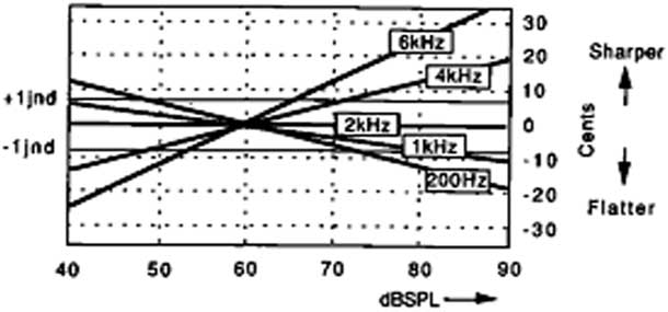
Sound example 1 also shows that, in spite of using the exact same frequency, the notes in the eight-note groups are perceived with micro-pitch variations. Although pitch perception is directly related to frequency, which is the basis for both place and temporal theories of pitch perception (Howard, David and Agnus Reference Howard, David and Agnus2001), changes in pitch may also occur by modifying its pressure level (see Section 3.1) while keeping the frequency constant. As shown in Figure 1, when varying the intensity between 40 dBSPL and 90 dBSPL while keeping the fundamental frequency (f) constant, a change in pitch is perceived for all f values other than those around 2 kHz. For f values greater than 2 kHz, the pitch becomes sharper, with increasing sound intensity; below 2 kHz the pitch becomes flatter as intensity increases. Rossing suggests a change of 17 cents (0.17 of a semitone) for an intensity change of between 65 dBSPL and 95 dBSPL, although he does not specify which type of signals and under which conditions this value is deduced (cited in Howard et al. Reference Howard, David and Agnus2001).

Figure 1 Pitch shifts perceived when the level of a sine wave with a constant fundamental frequency is varied.
Rossing also points out that the effect of intensity changes on pitch perception is especially relevant when using sine waves, and less noticeable when using complex sounds. This statement is borne out by the experiments realised here, as they show that using sounds with complex spectra drastically reduces the perception of sound attribute variations produced by the external ear. My experiments reveal, too, that pitch variations are especially important in differentiating the notes inside each note group, as was stated by Gabor: that pitch perception is one of the main mechanisms of microevent detection (Gabor Reference Gabor1946).
As our intention is to maximise the effects of sound localisation on sound perception, the sound material used in both experiments and compositions is tightly limited to sine waves. Time invariant sound signals with complex spectral components, such as square waves and triangle waves, are also used. However, they are restricted to situations where only one of such signals is presented at any one time. The experiments show that using several of such complex signals simultaneously creates monotonous and static situations, because sound spatialisation cannot imprint enough contrasting variations onto them. In contrast, by using simultaneous sine waves, as they occur within the compositions presented here, such variations are still perceivable.
3.3 Influence of note duration on pitch perception
Note duration has important consequences on pitch perception, as different numbers of cycles are needed for different fundamental frequencies so that a defined pitch can be perceived (see Figure 2). However, in spite of demanding fewer cycles, the duration of notes with low frequencies is longer compared to that of high frequencies, as its waveform needs more time to complete a cycle or period. For instance, while a tone with a frequency of 100 Hz requires 45 ms for the pitch fully to be perceived, a tone with a frequency of 1000 Hz requires only 14 ms (Butler Reference Butler1992).
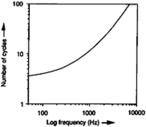
Figure 2 Effect of duration on pitch (from Rossing Reference Rossing1989).
The first consequence of decreasing the duration of the notes below its corresponding pitch threshold is that the notes are gradually perceived to be more non-pitched than pitched until heard as tone bursts. Tone bursts present a rich and complex spectrum, which implies that the subtle variations in pitch and loudness associated with sound spatialisation become much less evident. In addition, a short duration impedes the clear recognition of its sound quality variations produced by sound localisation: the more complex a sound, more time is needed ‘to establish a firm sense of the identity and properties of a microevent’ (Buser and Imbert Reference Buser and Imbert1992).
Another important consequence of using short note durations is that the position of the notes and their respective spatial trajectories become more relevant. In contrast, when pitch is more audible, attention is drawn more to the melodic contours. If we accept the theory that perceptual grouping is carried out by separate mechanisms (Deutsch Reference Deutsch1999), this experience may indicate that when listening to music, the mechanisms involved in evaluating pitch variations are more relevant than those evaluating sound location.
3.4 Influence of the reflections
Sound example 10 shows also how five-note groups with note durations of 1 and 6 ms are perceived as one clear note impulse followed by sound ‘rebounds’ of lower intensity. Given that the sound signals emitted by the notes occur together with the early reflections, it is here assumed that they may attenuate considerably its onset slopes, so they are perceived not as primary sounds but as echoes or extensions of previous sound events. This hypothesis gains consistency when analysing the echo thresholds, which depend not only on the time delay between the primary sound and reflections, but also on their level, angle of incidence to the ear, frequency, impulse width and the steepness of the onset slopes of the signal (Blauert Reference Blauert1997: 169). Similarly, Bregman’s studies also confirm the importance of the rate of onset on stream segregation (Bregman and Ahad Reference Bregman and Ahad1996: 47).
At the same time, the position of the primary sound event seems to coincide with the position assigned to the first note in the five-note group. However, reflections may also influence sound localisation. The auditory system takes into consideration coherent components of the ear input signals that arrive within two milliseconds after the first component so as to determine the position of the auditory events. This phenomenon, called ‘summing localisation’, may be especially important in determining the position not only of the first sound event, but also that of the echoes.
It is generally experienced, however, that when using note groups with short note durations, the positions of the first and last notes seem to be more prominent. Studies on grouping mechanisms corroborate this experience. They also confirm that, when using short note-groups, the first and last notes are perceptually more important than the middle ones (Bregman and Ahad Reference Bregman and Ahad1996: 36).
3.5 Other perceptual consequences of sound spatialisation
Sound spatialisation influences the morphological structure of the note groups in other ways besides merely its sound quality, localisation and extension. The dynamic movement of notes in space, for instance, creates spatial gestures with particular sound directionalities and sound trajectories. At the same time, depending on how the notes are organised in time and space, they mould particular spatial shapes, which are more evident when using individual note groups or a limited number of them, as is shown in Sound examples 9 and 10.
Sound spatialisation contributes also to achieve stream differentiation (Bregman Reference Bregman1990), especially relevant when the notes or note groups are not clearly differentiated through register or timbre. To improve stream segregation, this research introduces the ‘principle of no overlapping’. In this, simultaneous note groups cannot be radiated using the same loudspeakers. In addition, following the Gestalt principle of proximity (Koffka Reference Koffka1935; Wertheimer Reference Wertheimer1967), note groups are usually radiated using contiguous loudspeakers (see Figure 11(b)); they are grouped into different and differentiated spatial areas.
On the other hand, sound movement adds greater dynamism to the note groups, and this may lead to contradictory perceptual results: while increasing sound clarity, having the notes spatially more widely differentiated may cause difficulty in perceiving the totality of the temporal and spatial changes that occur simultaneously. This perceptual ‘blurring’ may be more evident when using short note durations, as the threshold for the correct perception of the ordering of a sequential pair of unrelated sounds is established at approximately 20 ms (Warren Reference Warren1999).
Finally, sound spatialisation may also create perceptual illusions. For instance, following Diana Deutsch’s ‘octave illusion’ or ‘scale illusion’ (Deutsch Reference Deutsch1999), when two identical notes sound successively in two different positions, as occurs constantly using eight-note groups, the second note could be dismissed when a third note happens simultaneously with the second one at another position. At the same time, the perceived location of such notes might also be misplaced, for instance, according to pitch range similarities. As Deutsch’s experiments use dichotic listening, it is assumed that similar unpredictable (illusory) situations in relation to sound perception and sound localisation might occur when eight sound sources are placed around the listener.
3.6 Summary
The previous theoretical background demonstrates that real space may be used to manipulate the perception of sound at micro-timescales. Of fundamental interest to this research is that all variations explained above occur through the interaction of sound with reality, namely, through the effects of resonance, absorption and reverberation produced by the physical (acoustic) space, the body and the auditory system. This approach implies a clear differentiation when compared to electronic music in general and, more precisely, to granular synthesis; this is where sound is transformed mainly according to fictive interactions with virtual spaces, using spatial algorithms such as electronic delays, spectral filters, panoramic motion and reverberation applied to each sound grain (Roads Reference Roads2001: 236).
The relation and dependence of sound perception on the distortions produced by physical realities demonstrates similarities with, for instance, the ‘body related sculptures’ by the sound artist Bernhard Leitner, where sound interacts with the movement and physicality of the body to create ‘audio-physical experiences’ (Leitner Reference Leitner2008: 135). Maryanne Amacher’s Sound Characters (Making the Third Ear), in which ‘the rooms themselves become speakers, producing sound which is felt throughout the body as well as heard’ (Amacher Reference Amacher1999) is another example. Both artists conceive the human body as a ‘resonant space … in which aural structures can develop’ (Ouzounian Reference Ouzounian2006). This research, however, tries to find strategies where these types of interactions may be implemented within a more time-based musical discourse.
4 SOUND SPATIALIsATION: OLD AND NEW STRATEGIES
The next step consists of creating middle- and large-scale musical structures as gestures and textures in such a way that the capacity to perceive the distortions that the auditory system, body and acoustic space imprint on the sound are still detectable. Therefore, the same note groups used in the experiments are used as basic structural elements of longer sonic structures. The following procedures resemble in many aspects Gabor’s decomposition of a sound into micro-acoustic ‘quanta’ (Gabor Reference Gabor1946) or Xenakis’s strategies using sound grains. However, the need to preserve the variations that sound localisation imprints onto sound perception demands the implementation of new approaches.
The strategies proposed here follow three essential steps. First comes the division of sine waves into small units called ‘notes’. The amplitude envelope of these notes contains three phases: attack, sustain and release. The attack and release consist of very short fade-in and fade-out envelopes, not intended to give any particular shape to the sound, but to prevent undesired clicks or tone bursts.
Second, the resulting sound units are organised into five-note groups and eight-note groups. The maximum number of notes in one group coincides with the number of loudspeakers used during the experiments, thus each note can be radiated from either five or eight different angles in relation to the ears. The main difference between the five-note groups and the eight-note groups is that the former use notes with different frequencies, while the latter use notes with the same frequency.
The creation of upper structures is the result of repeating several (identical) note groups in succession. These structural processes recall Xenakis’s method of using sound grains, as he created long sound structures by scattering grains into ‘time-grids’, called ‘screens’, and playing sequences of ‘screens’, which he called ‘books’. A book of screens could be used to create long and complex clouds of grains in evolution (Xenakis Reference Xenakis1960).
However, instead of using screens containing hundreds of sound grains, sound units are here organised into groups of five or eight units. This is an important difference, because their organisation in time and space can be made manually through micromontage, as is explained later. In contrast, the distribution of grains on a screen to create sound clouds, sound masses or textures usually applies statistical methods, such as the probability theory, that require automated processes (Xenakis Reference Xenakis1971; Roads Reference Roads2001).
4.1 Sound-space density
Third, sound units are organised in space following different sound-space densities, which result from using a different number of loudspeakers. Sound-space densities are represented by two integers in parentheses: the first integer describes the total amount of notes in the note group, while the second integer shows the quantity of loudspeakers used. Figure 3 illustrates two opposite sound-space density situations: while in (a) one loudspeaker radiates eight sound units (sound-space density (8,1)), in (b) eight loudspeakers radiate eight sound units (sound-space density (8,8)).
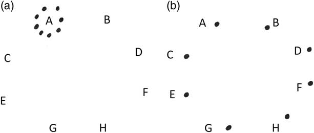
Figure 3 Graphic representation of sound-space densities: (a) (8,1) and (b) (8,8).
Sound example 3 shows how a continuous tone consisting of successive (identical) eight-note groups is perceived with constant sound quality, rhythm and texture variations while passing through different sound-space densities.
It is important to mention that the possibility to manipulate sound ‘density’ through applying different sound-space densities represents a fundamental difference from other methods using sound particles. In granular synthesis or Xenakis’s use of grains, for instance, density variations imply changing the number of grains per unit time, the duration of each, or the time intervals between them (Roads Reference Roads2001). Here, however, density variations refer to the arrangement of sound units in space using a greater or smaller number of loudspeakers, while the other parameters, that is, sound duration, amount of notes per unit time, and time intervals between the notes, remain invariable.
5 ORGANIsING THE NOTES IN TIME AND SPACE: METHODOLOGY
Before explaining in detail how note groups are organised so as to create dynamic textures and gestures, it is necessary to explain that the micromontage was conducted using Pro Tools. This audio workstation (DAW) offers a three-dimensional work-space that includes tracks, time and space. The main reason for choosing this method was that at the beginning of this research it was convenient to work directly on each note, to control the precise quantity, duration and position, and to visualise each process. Working in this way prevents any kind of computer programming as an intermediate step.
5.1 Assigning the notes into tracks and loudspeakers
Using Pro Tools, the temporal and spatial organisation of the notes requires two steps. First, the eight notes are organised in relation to eight independent tracks. During the experiments, it was observed that successively repeating the same track positions created recurrent rhythms and sound trajectories; these were particularly frustrating in short note durations. To prevent these repeated patterns, I created eight (O) rows with different arrangements of the notes in relation to the tracks, then realised three variations of these rows, called retrograde (R), inversion (I) and inversion plus retrograde (IR). These rows alternate from both right to left and from front to rear aural regions, ensuring greater perceptual contrasts and non-repetitive sound trajectories. Figure 4 shows eight (O) and (IR) rows. Note that both the sequence of the rows and the numbers inside each row are, in the (IR) rows, played backwards compared to the eight (O) rows.

Figure 4 (O) and (IR) rows corresponding to the position of the notes in the tracks.
The rows are divided in two groups of four digits to facilitate their recognition. The eight digits of each row correspond to the eight successive notes in the eight-note groups, while the numbers 1, 2, 3, 4, 5, 6, 7 and 8 assigned to them correspond to the eight succeeding audio tracks (Aud 1, Aud 2, etc.). Figure 5 shows the arrangement of (O) rows in their track positions as they appear in the Pro Tools session.
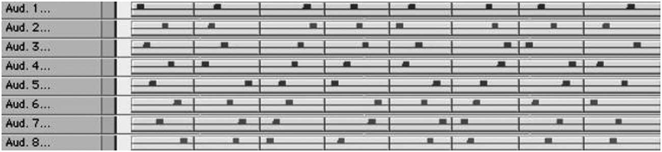
Figure 5 Graphic illustration showing the arrangements of the notes in relation to the audio tracks following the 12 (O) rows.
The tracks are then assigned to particular loudspeakers according to their different sound-space densities. As the use of contrasting aural locations and sound-space densities proved to increase the perception of rhythm and texture variations, I also created sound-space density rows (see Figure 6).
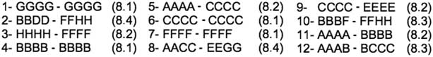
Figure 6 Example of 12 rows with particular loudspeaker arrangements.
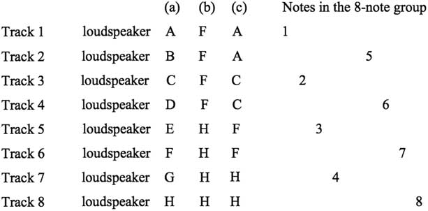
Here, the eight digits represent the eight audio tracks: the first digit corresponds to the first audio track, the second one to the second audio track, and so on. The letters A, B, C, D, E, F, G, and H correspond respectively to the eight loudspeakers (see Figure 3).
5.2 Examples of different sound-space densities
The organisation of the notes into tracks and loudspeakers as proposed here permits the organisation of the notes in both space and time, as a particular loudspeaker is assigned to each successive note in the eight-note groups, that is, their position in space; simultaneously, they establish which speaker sounds first, that is, the chronological order. To illustrate this relation, I include several examples.
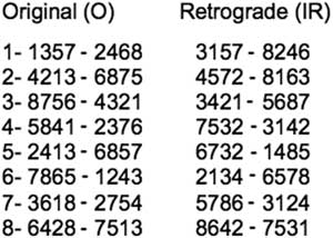
In the first example, the notes are organised following the track position 1357–2468 and loudspeaker arrangement ACEG-BDFH (see Figure 7(a)), thus using sound-space density (8,8).

Figure 7 Examples showing the relationship between track position and loudspeaker arrangement.
The movement of sound in time and space describes two identical sound trajectories: the four sound sources at the left hemisphere describe a front-to-rear movement first, followed by the four sound sources at the right hemisphere (see Figure 8).
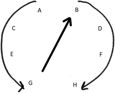
Figure 8 Front–rear movement described by the (O) track position row n.1.
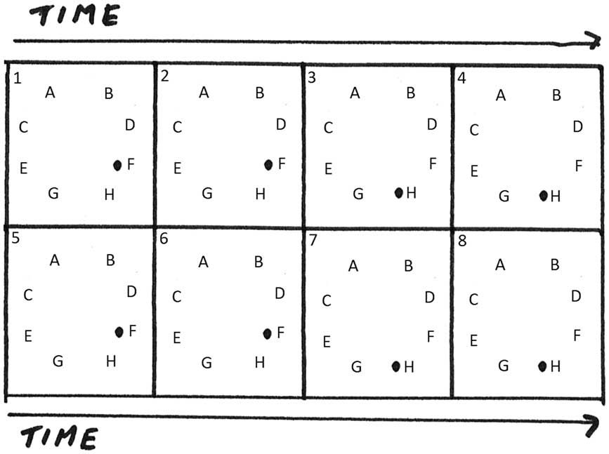
In the second example, the previous track position 1357-2468 remains invariable, while the loudspeaker arrangement changes to FFFF-HHHH (see Figure 7(b)). The previous sound-space density (8,8) becomes (8,2), reducing drastically the spatial extension, thus the perception of the same track position is distinguished from the previous example: first, two notes appear at loudspeaker F, then two notes at loudspeaker H, followed by two notes again at loudspeaker F, and two at loudspeaker H (see Figure 9).

Figure 9 Graph of the temporal and spatial organisation of the notes in the eight-note groups using track position 1357-2468 and loudspeaker arrangement FFFF-HHHH. The numbers associated with each position indicate the temporal succession of the sound events.
In the third example, the loudspeaker arrangement changes to AACC-FFHH (see Figure 7(c)) while keeping once again the same track positions 1357-2468. In this case, the first two notes appear at speakers A and C, followed by two notes at loudspeakers F and H. The next four notes repeat the same temporal and spatial movement (see Figure 10).

Figure 10 Graph of the temporal and spatial organisation of the notes in the eight-note groups using track positions 1357-2468 and loudspeaker arrangement AACC-FFHH.
As can be seen, each sound-space density creates particular spatial gestures, sound directionalities and sound trajectories; these, together with the perception of particular sound quality, rhythm and texture variations, allow the differentiation of identical eight-note groups.
5.3 Spatial width
Sound-space density defines the spatial extension of particular note groups, as notes are spread in space using a variable number of loudspeakers. However, identical sound-space densities can use adjacent or distant loudspeakers, altering considerably the spatial width of a note group. For instance, sound-space density (8,2) could be radiated using either two adjacent loudspeakers, that is, speakers (AAAA-BBBB) or two located at a distance (AAAA-HHHH).
6 THE CREATION OF MUSICAL STRUCTURES
Depending on the note-group typology (as is defined by its sound signal, frequency, note duration and time intervals between notes and note groups), the amount of repeated note-groups and the sound spatialisation strategy used, it is possible to create different types of mesostructures, here classified into two main categories:
1. Textural, including sustained tones and continuums.
2. Gestural, including attacks and sound objects.
6.1 Sustained tones
Sustained tones (Sound example 4) represent the most invariable long continuous tone, as they consist of successive (identical) eight-note groups with the same sound signal, frequency and note duration. The time interval between notes and note groups is always 0 ms. At the same time, they always use sound-space density (8,8) and therefore experience no rhythm or texture changes.
However, sustained tones use note durations beyond the pitch thresholds that facilitate variations in the perception of pitch and loudness. As observed and described in Section 3, low frequencies use longer note durations compared to those of high frequencies, which allows a listener more clearly to perceive and differentiate each note and follow the spatial trajectories they create. When several sustained tones are played together, as in the composition Musical Situation 1, these dynamic sound trajectories contrast with the non-directional diffuse sound fields created by higher frequencies.
If the two versions of the same sustained tone in Sound example 4 are compared, at least two important differences are perceived. First, the ‘rough’ quality heard when using one channel, similar to a tremolo, disappears in the octophonic version. The reason may be that the onset of each individual note is largely masked due to the reflections. When the onset is attenuated (see Section 3.4), the transition between two adjacent notes is smoother, and the ‘rough’ quality disappears.
Furthermore, sound spatialisation increases the level of depth and diffusion of the sound field, which vary depending on the amplitude level of the primary sounds. Sound example 13 (m. 2′54″), for instance, shows how sound depth increases while lowering the amplitude of the sustained tones, as soon as the level of the primary sounds equals the level of the reflections.
6.2 Continuums
Continuums use shorter note durations (c. >50 ms) compared to sustained tones, and the time intervals between the notes and note-groups are larger than 0 ms. When note duration is very short, the individual notes are perceived as tone bursts. In these situations, the larger time intervals between the notes imply that the continuums are perceived as transparent lines made of short points (sound impulses) (Sound example 2). When using short time intervals, however, transparency is lost, favouring a more dense sound with particular grades of opaqueness depending on the time intervals between the notes (Sound example 3).
At the same time, the notes follow one another at different speeds according to each note’s duration and the time intervals between them. Higher speeds produce the perception of a pitched quality that is related not to the frequency of the notes, but to the repetition period (Roads Reference Roads2001: 105). For instance, Sound example 5 shows five successive eight-note groups consisting of a 408 Hz triangle wave, with a note duration of 3 ms, and time intervals of 250, 125, 65, 30 and 15ms respectively. As the time intervals decrease, the velocity of note succession increases, and the eight-note groups create an outstanding pitched tone that emerges together with a more prominent ‘rough’ quality.
Continuums are divided into two groups: homogeneous and heterogeneous. Homogeneous continuums represent the most uniform continuum possible. This occurs because they use consecutive (identical) eight-note groups, with the same sound signal, frequency, note duration and synchronous (same) time intervals between notes and note groups. The only parameter that varies is sound-space density (Sound example 6). Heterogeneous continuums are less uniform in that they use the same consecutive (identical) eight-note groups but with asynchronous time intervals. At the same time, they incorporate the transient sounds that occur naturally when the fade-in and fade-out envelopes of each note are removed, adding an additional ‘rough’ quality to the notes (Sound example 7).
In spite of using variable time intervals between notes and note groups, heterogeneous continuums are perceived to have a uniform sound quality. The reason is that the time interval variations are too small and the note duration too short to create rhythm and texture variations, although these aspects may affect its ‘roughness’. Despite alternating two sound qualities, that is, with or without fade-in/fade-out envelopes, each one remains uninterrupted long enough to facilitate its recognition and subsequent perceptual analysis (Bregman and Ahad Reference Bregman and Ahad1966: 74).
6.3 Sound objects
Sound objects consist of short sound structures (c.1 to 4 sec) using either five-note groups or eight-note groups successively. Sound example 8, for instance, presents 11 polyphonic sound objects created using four short mesostructures, all using eight-note groups with the same sound material (sine wave), frequency (159 Hz), and note duration (1 ms); however, they have different time intervals (0, 6, 23 and 92ms), both between notes and note-groups, which feature imprints a particular sound quality and texture that helps in distinguishing them.
To achieve greater sound clarity, they are nevertheless arranged in space using adjacent loudspeakers following the ‘principal of no overlapping’ explained in Section 3.5 (see Figure 11). Also, some are played at different times. This strategy follows the ‘old-plus-new’ heuristic (Bregman and Ahad Reference Bregman and Ahad1996: 56), which shows how preattentive mechanisms help to capture (and recognise) sounds from a mixture.

Figure 11 Graphic representation of sound objects 7 and 8 in Audio Example 8. Graphic (a) represents the temporal organisation of each mesostructure and its duration, while graphic (b) shows its spatial arrangement. The numbers 0, 6, 23 and 92 represent the time intervals.
Sound example 9, in contrast, presents sound objects that result from playing different amounts of identical five-note groups. These note groups consist of sine waves with five of the following frequencies: 53, 159, 212, 318, 477, 795 and 954 Hz, with note durations of 1, 6, 11, 23 or 46 ms, and different note and note-group time-intervals. The purpose of using note groups with different frequencies is more optimally to differentiate the notes in the note-groups, especially when using short note durations. When note durations are very short, however, using different frequencies has little influence on the sound quality, as this depends strongly on note duration (see Section 3.3).
6.4 Individual note groups
Depending on their note duration, individual note-groups are perceived either with micro-melodic contours, as short sound objects which create spatial gestures with particular sound trajectories and sound directionalities, or as one unique sound impulse or attack followed by more or fewer echoes (see Section 3.4). Sound example 11 illustrates all these possible scenarios, as it presents five series of approximately eight individual eight-note groups, consisting of a 408 Hz sine wave, with note durations of 250, 130, 60, 30 and 15 ms respectively, and time intervals of 0 ms.
7 COMPOSITIONS
Some of the mesostructures created during the experiments are used to compose three pieces, each one experimenting with different types of musical structures. For instance, the piece Topos (3′) (Sound example 12) is based principally on attacks, sound objects and short continuums, changing constantly and rapidly over time. Despite all these variations, the consequences of sound spatialisation and sound-space density changes are still perceptible, and contribute significantly towards accomplishing a rich and dynamic musical discourse. Nevertheless, every attempt to construct a larger musical piece was in vain. I presume that working with gestures demands the use of sounds with a richer and more variable spectrum than the time-invariant sound signals used here. At the same time, it may be necessary to change other (temporal) parameters to achieve more dynamic and contrasting gestures, which cannot be accomplished when using sound-space density variations only.
In contrast, Musical Situation 1 (22′) and Polyphonic Continuum (10′) demonstrate that sustained tones and continuums permit the creation of long musical discourses. The non-existence of primary impulses creates the sense that energy is dilated in time, permitting attention to concentrate on the inner activity of sound instead of the forward motion (Smalley Reference Smalley1997: 112). In this sense, sound spatialisation and the use of sound-space density variations enormously enrich the inner structure of textures, as they imprint multiple and dissimilar sound quality, rhythm and texture variations. As is explained later, the natural causes that lay behind these variations are also fundamental to imprint a particular ‘aura’ to sound that increases substantially its interest (see Section 8).
Sound example 13, for instance, shows the first three episodes of Musical Situation 1. The sound material is exactly the same for all three episodes, consisting of four sine waves with frequencies of 53, 159, 212 and 318 Hz, respectively. These frequencies are first played as a harmonic chord on one channel at the very beginning, followed by the corresponding sustained tones also played on one channel. Note how the sterile, flat and invariable harmonic chord is gradually transformed into a more complex, ambiguous and interesting musical structure as soon as the notes are spread in space. Note also how different the perception of spatial depth is as soon as the sustained tones are spatialised. At the end of the first and third episodes, the sustained tones disappear gradually one after the other, such that the remaining tones are promptly more prominent, and it is easier to follow the sound quality and sound location variations of each. In addition, sustained tones include passages that lack the fade-in/fade-out envelopes, creating a granular surface above the diffuse sound field.
Sound example 14 presents two sections of the piece Polyphonic Continuum: the first consists of three continuums with frequencies of 53, 318 and 477 Hz; the second includes five continuums with frequencies of 53, 212, 318, 477 and 795 Hz. Differently to Musical Situation 1, where the individual layers are not clearly segregated (see Section 3.5), in Polyphonic Continuum it is possible to perceive each layer and follow the sound quality, texture, and rhythm variations associated with the movement of sound through different locations and sound-space densities. As opposed to sustained tones, continuums use shorter note durations and different time-intervals between notes and groups, which factor implies that the onset of the notes is much more pronounced. Also, each continuum presents a differentiated frequency and texture, which benefits stream segregation and assists in the recognition of the spatial movement of each individual continuum and the perceptual variations associated with it.
Finally, the long duration of each continuum facilitates recognising and differentiating them, confirming Bregman’s assessment that longer unbroken sequences segregate more easily than do shorter ones (Bregman and Ahad Reference Bregman and Ahad1996: 18). This is especially true in the last episode of Sound example 14, where five continuums are played simultaneously from the very beginning. Note that a certain period of time is required until it is possible to segregate sound into multiple streams, and how sound movement, together with amplitude variations (see Section 9), contribute to distinguishing them.
8 THE PERCEPTION OF CAUSE-EFFECT RELATIONS: ‘GESTURAL SURROGACY’
Smalley considers the possibility of generating sounds detached from their physical gestures, which he calls ‘gestural surrogacy’, as one of the main achievements of electronic music, permitting the full achievement of a ‘reduced listening’ (Schaeffer Reference Schaeffer1966: 270–2). I consider that the strategies presented here achieve a certain degree of gestural causality, despite the use of electronically generated sounds. On the one hand, even though it is not possible to relate them to any original source, their perceptual variations are attached to specific ‘natural’ causes, namely, the distortions produced when interacting with the real (acoustic) space, the subject’s body and the psychophysics of human sound localisation.
On the other hand, if we consider gesture as an ‘energy-motion-trajectory which excites a sounding body creating spectromorphological life’ (Smalley Reference Smalley1997: 111), it is not less true that sound movement is here the agent that provokes perceptual variations to a given sound. Sound examples 13 or 14, for instance, show how a static harmonic chord is brought into ‘morphological life’ by moving its small units in space following different positions and sound-space densities, producing sound quality, rhythm and texture variations.
I am convinced that the listener may have the impression, although probably only intuitively, that there is a relationship between sound movement and the sound variations he or she perceives. Comprehending that these variations obey particular spatial gestures, namely, the concentration and dispersion of sound unities (energy) in space that occur together with sound-space density variations, is relatively straightforward. In addition, I am also convinced that there are qualitative sound characteristics inherent in the naturally created sound fields that clearly differentiate them from those created artificially.
9 THE IMPORTANCE OF AMPLITUDE VARIATIONS
Amplitude variations proved to be an extremely powerful variable that helped to invigorate the musical structures in many different ways. In contrast to frequency and timbre variations, which attract our attention to melodic patterns, varying the amplitude does not mask the cause–effect relations between sound movement and the perception of sound attribute, rhythm and texture variations. This is especially true when the curve of the amplitude envelope is smooth enough to create any attack or decay that could be perceived as an abrupt gesture.
Sound example 14 shows how subtle dynamic changes permit particular continuums momentarily to be more prominent than others, thus achieving a more dynamic polyphonic situation by continuously creating new sound contours and reliefs. Sound example 13, in comparison, shows how gradual amplitude changes create completely different textures, tone colours and spatial depths, using exactly the same four sustained tones.
10 THE PERCEPTION OF EXCEPTIONAL DIFFUSE SOUND FIELDS
Another important consequence of using amplitude variations is the possibility of reaching different grades of sound diffusion. Although diffuse sound fields normally occur in large reverberant halls when the reverberations mask the onset of the primary sounds, here they happen independently of the reverberation levels of the room. Why do these ‘exceptional’ sound fields occur?
On the one hand, the large amount of small sound units with an identical sound signal, frequency, and note duration, radiated from different positions in space at very short time intervals, may generate an ‘exceptional’ number of reflections. Those specific distortions occurring when sound reaches the external ear may also contribute in creating such sound fields, as each primary sound is distorted differently depending on the angle of incidence to the ears. The superposition of an extraordinary amount of primary sounds and reflections with different degrees of incoherence may increase significantly the level of the reverberation. The composition Musical Situation 1 shows how sound diffusion is particularly high when the amplitude level of the primary sounds is lowered to the point that it equals the level of the reflections (as these occur in Sound example 13 (2′30″)).
The possibility to create such sound fields is very important for this research, as they result in achieving sound perspective and spatial depth, two sound properties of fundamental importance in electronic music, without using any artificial reverb. Far from being artificial, their amount and quality is directly related to – and cannot be considered separately from – specific types of sound signals, specific amplitude levels, such specific strategies in relation to sound spatialisation, with particular interactions between the primary sounds and the reflections created by the acoustic characteristics of the room. This also involves the psychophysical processes of sound localisation.
11 CONCLUSIONS
The elemental quality of sine waves and other time-invariant sound signals brings to the foreground sound distortions produced by the environment, our bodies and our auditory systems; these usually remain inaudible due to the (spectral) complexity and variability of the sound signals, on the one hand, and the temporal manipulations they experience during the compositional processes of a musical piece, on the other. This research presents three essential strategies that allow the creation of dynamic musical structures where these sound distortions are still audible: the use of time invariant sound signals, their division into small units, and their spatialisation according to different sound-space densities.
Through these strategies, the movement of sound in space becomes the primary, and sometimes the sole, parameter to generate morphological variations of sounds and musical structures, including the perception of variations in pitch and in loudness; the creation of variable and dynamic rhythmic structures, texture qualities and spatial gestures; and the possibility to achieve different levels of spatial depth independent of the levels of reverberation of the acoustic spaces. The main purpose of this research, which was to increase the importance of sound spatialisation in musical composition, is thus achieved.
Another important accomplishment of this research is that electronically generated sounds overcome, to a certain degree, their artificiality: they are transformed and enriched according to specific physical and psychophysical processes that occur when they interact with the acoustic space, the body and our auditory system. Even more important is the fact that these variations occur at the precise moment of the performance of the piece. This immediacy imparts to electronically generated sounds a level of vitality and authenticity unusual in electronic music.