


1. Introduction
Sentiment analysis is the task of identifying and categorizing opinions by automatic methods, which are expressed in a piece of text by a reviewer about an entity or a topic. This problem has recently gained popularity due to its vast use in many areas, such as social media analysis, marketing, and customer service. In English and other widely-used languages, there are many well-established sentiment lexicons, such as SentiWordNet (Baccianella, Esuli, and Sebastiani Reference Baccianella, Esuli and Sebastiani2010), and large-scale labeled corpora. However, this is a challenging task for other languages that lack such hand-curated dictionaries and datasets.
An important issue that should be taken into account when developing applications in this field is that a sentiment word may carry a negative or a positive connotation depending on its context or domain. For example, the word “loud” may have a negative sentiment in a car review, but it could have a positive sentiment in a headphone review. It is also possible that, across languages, the polarities of some words can change. In order to overcome these problems, lexicon-based or domain-based techniques need to be developed.
In this paper, we focus on the binary sentiment classification problem for Turkish at document level. We make a comprehensive analysis and propose a framework that includes unsupervised, semi-supervised, and supervised methods, as well as the combination of these methods. The unsupervised and semi-supervised approaches we have developed can be used in domain-specific and domain-independent contexts. Our work is the first one that takes into account the domain-independent approach in sentiment analysis for Turkish, to the best of our knowledge. Apart from this, we adopt different feature engineering techniques and we feed them as input into the machine learning methods. Lastly, we combine the supervised features with the unsupervised features. The combined feature set improved the success rates in most of the cases.
We applied the proposed methods to a movie reviews dataset and a Twitter dataset in Turkish. The reviews dataset is the dataset used in a previous work (Türkmenoğlu and Tantuğ Reference Türkmenoğlu and Tantuğ2014) which we refer to as a baseline study for comparison. The Twitter dataset was compiled in this research, and the tweets were annotated by two annotators. The methods improved the baseline results with a significant margin for the movie dataset. We observed that the selection of the “right” feature set has a higher impact on performance than the choice of the machine learning algorithm. We also evaluated the proposed approaches on three datasets in English and obtained significant results. Our system can be applied to other languages as well with minor changes. The source code is publicly available.Footnote a
The research objective in this study is building a framework that can identify the sentiments of Turkish text with high success rates. Based on this motivation, we address a number of research questions. Does comprehensive preprocessing and morphological analysis contribute more than the specific sentiment model for morphologically rich languages? What is the effect of utilizing sentiment lexicons generated in an unsupervised or a semi-supervised manner on the performance of the system? Does combining unsupervised, semi-supervised, and supervised methods lead to higher success rates? Lastly, can classical machine learning algorithms fed with effective features outperform neural network models?
The rest of the paper is organized as follows. In Section 2, we present the existing works on sentiment classification in Turkish and other languages. In Section 3, we describe the proposed approach. The experimental results are shown and the main contributions of the proposed approach are discussed in Section 4. In Section 5, we conclude the paper.
2. Related work
Unsupervised approaches: There are several studies that obtain the sentiments of sentences or documents based on the sentiments of words in an unsupervised manner. In the work of Turney (Reference Turney2002), polarity scores of words and phrases are extracted using a search engine. The documents are then classified based on the average semantic orientation of the phrases it contains. The accuracies obtained for the movie domain were lower (66%) compared to the banks and automobiles domains (80–84%). In our work, we adopted the same approach with some changes such as using a different set of query words and operators on movie reviews and Twitter datasets in Turkish. It was also reported that the search engine results are sometimes erratic and the use of a static corpus might be better (Taboada, Anthony, and Voll Reference Taboada, Anthony and Voll2006). We utilized static corpora as well for our semi-supervised method in a different manner. Another prominent study that affected the sentiment analysis field is the work of Hatzivassiloglou and McKeown (Reference Hatzivassiloglou and McKeown1997). They extract sentiment information on a word basis by focusing on adjectives.
Semi-supervised approaches: Resources that incorporate sentiment information are frequently used in sentiment analysis studies. In Hamilton et al. (Reference Hamilton, Clark, Leskovec and Jurafsky2016), a sentiment lexicon is induced using a semi-supervised approach. The intuition in this study is that choosing a few sentiment words manually specific to a domain may help find the sentiment labels of other words in an unlabelled corpus. We also used this algorithm in the domain-specific model built in this work by adjusting the model parameters. Another study (Martinez-Camara et al. 2014) combines the unsupervised and supervised approaches for sentiment analysis by making use of sentiment lexicons. The main drawback of this study is its not being domain-adaptable, unlike the approach we propose.
Supervised approaches: Besides these unsupervised and semi-supervised approaches on word basis, most studies focus on supervised learning schemes and extract sentiments on a review basis. The supervised approaches mostly utilize boolean or tf-idf (term frequency—inverse document frequency) metrics as a weighting scheme (Li and Liu Reference Li and Liu2010; Yıldırım et al. Reference Yıldırım, Çetin, Eryiğit and Temel2014). In a few works (Martineau and Finin Reference Martineau and Finin2009), the delta tf-idf metric is used, and it proves to be more useful as compared with the boolean and tf-idf schemes. We use similar metrics which take into account the characteristics of the polarity classes. Another study extracts three polarity scores for each word in a review, and it achieves a higher success rate (Farhadloo and Rolland Reference Farhadloo and Rolland2013). In one of the weighting schemes we use, we make use of a similar technique in the sense that we extract the most indicative three polarity scores of each review. Related to the Twitter data, Santos and Gatti (Reference Santos and Gatti2014) utilize some extra features, such as character n-grams, and show that it helps overcome the problem of data sparsity in sentiment analysis. Other features, such as POS (part-of-speech) tags, minimal and maximal sentiment scores in a review, and the number of emoticons are also taken into account (Lango, Brzezinski, and Stefanowski Reference Lango, Brzezinski and Stefanowski2016).
In Thelwall, Buckley, and Paltoglou (Reference Thelwall, Buckley and Paltoglou2012), repeated letters and punctuation marks in the text are reported to boost the strength of the immediately preceding sentiment. Wang and Manning (Reference Wang and Manning2012) show that bigram features can capture modified verbs and nouns. Therefore, employing these in the sentiment classification task yields a better performance than the “bag of words” model. An approach (Guha, Joshi, and Varma Reference Guha, Joshi and Varma2015) relies on the presence or absence of some words when performing aspect-based sentiment analysis. For example, the presence of wh-words and conditional words, such as “what” and “if,” are mostly characteristic of sentences and reviews of negative polarity.
As a supervised domain-specific approach, Jiang, Lan, and Wu (Reference Jiang, Lan and Wu2017) perform fine-grained sentiment analysis on the domains of news headlines and financial microblogs. They utilize four types of features, which are sentiment lexicon features, linguistic features, domain-specific features, and word embeddings. As domain-specific features, they use numbers, metadata, and punctuation marks. For example, when a number is preceded by the “+” sign, it most likely is a positive indicator in the finance domain. When they employ ensemble regression models, they achieve comparatively high performance. We instead manually choose polarity seed words per domain and do not extract domain-specific rules per review to feed them as input into the supervised approaches. Saroufim, Almatarky, and Abdel Hady (Reference Saroufim, Almatarky and Abdel Hady2018) generate sentiment-specific embeddings that are language-independent. They employ a supervised component on top of a word2vec model. Emojis and emoticons are used to auto-label a large corpus of tweets. They thereby outperform the word2vec approach. They also propagate those labels in a graph to build sentiment lexicons.
Among the supervised approaches, support vector machines (SVM) are commonly preferred due to its ability to avoid overfitting using the kernel trick and being defined by a convex optimization problem where the issue of local minima does not occur (Wang and Manning Reference Wang and Manning2012). Besides, deep neural networks (DNNs) have recently gained popularity in many domains due to their accuracy, efficiency, and flexibility. Whereas most of the traditional machine learning algorithms require quite an effort and intense time to extract features by which to classify the data, these features can be created automatically by DNNs. Deep neural architectures have been applied to the sentiment analysis problem in some studies using word embeddings, such as word2vec (Mikolov et al. Reference Mikolov, Chen, Corrado and Dean2013). In Maas et al. (Reference Maas, Daly, Pham, Huang, Ng and Pott2011), the supervised scores of movie reviews are used and sentiment-aware embeddings are generated. Utilizing not only the semantic but also the sentiment information of words when creating word vectors boosts the performance of their model. We follow a similar approach such that we combine the supervised and unsupervised characteristics of the words. However, we do not generate sentiment-aware embeddings in this work. In a recent study (Felbo et al. Reference Felbo, Mislove, Søgaard, Rahwan and Lehmann2017), emojis are used to extract emotions from tweets via distant supervision and a bi-LSTM (bidirectional long short-term memory) framework is built to perform multiclass sentiment classification. They also detect sarcasm in reviews using a slightly modified version of this neural network. Baziotis, Pelekis, and Doulkeridis (Reference Baziotis, Pelekis and Doulkeridis2017) perform message-level and topic-based sentiment analyses separately. They employ a two-layer bi-LSTM model with attention over the last layer for the message-level classification task. For the topic-based classification part, a “Siamese” bidirectional LSTM is developed with a context-aware attention mechanism. They do not use hand-crafted features or sentiment lexicons in this study. Despite this, they ranked first (tie) in the Subtask A of the SemEval 2017 competition.
Studies in Turkish sentiment analysis: In Turkish, mostly the supervised approaches are used for sentiment analysis. Kaya, Fidan, and Toroslu (Reference Kaya, Fidan and Toroslu2012) apply sentiment classification to Turkish political columns using maximum entropy, n-gram language model, SVM, and naive Bayes (NB). All the approaches reached accuracies ranging from 65% to 77%. In Çetın and Amasyalı (Reference Çetin and Amasyalı2013), active learning is implemented for the Twitter dataset in Turkish, using a weighting scheme similar to ours. In the work of Türkmenoğlu and Tantuğ (Reference Türkmenoğlu and Tantuğ2014), an English sentiment lexicon is translated to Turkish and some supervised methods are employed. They also utilize bigram features in addition to unigrams in their models. They state that making use of the absence and presence suffixes in Turkish brings reasonable improvement to the performance. They obtained an accuracy of 89.5% in this study. The works in Turkish that develop unsupervised or semi-supervised methods either translate English lexicons into Turkish (Vural et al. Reference Vural, Cambazoğlu, Şenkul and Tokgöz2012) or create polarity lexicons based on corpora (Dehkhargani et al. Reference Dehkhargani, Saygn, Yanıkoğlu and Oflazer2016). An approach as in Turney (Reference Turney2002) has not been implemented for Turkish using search engines. To the best of our knowledge, the current work is the first one that employs this approach. Also, the studies carried out for the sentiment classification task in Turkish utilize only the root forms of words and a few number of affixes, such as the negation morpheme. By contrast, we perform a comprehensive morphological analysis and we show that using not only the root forms and the negation morphemes but also the other morphemes in a supervised manner can help boost the performance for sentiment analysis in an agglutinative language.
Other morphologically rich languages: In Abdul-Mageed, Diab, and Korayem (Reference Abdul-Mageed, Diab and Korayem2011), inflectional and derivational suffixes are not ignored and are used in the sentiment classification task for Arabic. Including these features and employing the SVM algorithm for binary classification yielded better F1-scores, compared to utilizing only the stems of the words. Joshi, Bhattacharyya, and Balamurali (Reference Joshi, Bhattacharyya and Balamurali2010) implement a three-stage system for extracting sentiments from reviews for the Hindi language. In this study, if an annotated corpus exists for the language, classification is performed using a supervised algorithm. If no such corpus exists, machine translation is employed to translate reviews into English and sentiment classification is carried out in this language. Lastly, if none of those approaches can be used, a sentiment lexicon is created for Hindi taking account of its morphologically rich structure, and reviews are classified using a majority voting scheme. In the work of Yang and Chao (Reference Yang and Chao2015), seed words and Chinese morphemes, which are mono-syllabic characters, are utilized to classify movie reviews without using any sentiment resources. The studies mentioned here do not use the surface forms of the words since this would largely increase the size of the feature set. They instead utilize some specific suffixes of the words in terms of additional features. Similar to these works, we also extract morphological features from the words and test the effects of different combinations of these features.
In Jang and Shin (Reference Jang and Shin2010), a sentiment analysis framework is developed for Korean. In this study, some Korean morphemes that are indicative of sentiments are used in addition to the root forms. They use sentiment lexicons and annotated datasets for classifying movie reviews. They also utilize a chunking method based on the dependency relations between morpheme sequences. For instance, negation shifters influence only the elements in the same chunk. We also follow a similar approach that uses a subset of all the morphological features. We employ negation shifters and other contextual features as well. In the work of Medagoda (Reference Medagoda2016), machine learning approaches are used to classify reviews in a morphologically rich language, Sinhala. He analyses how the selection of appropriate adjectives and adverbs affects the success rates for the classification task. The polarity scores are generated using different weighting schemes. Medagoda (Reference Medagoda2017) proposes approaches for generating sentiment lexicons for the Sinhala language. First, a cross-lingual method is employed by taking account of a sentiment lexicon for English and a basic dictionary of the target language. Second, a sentiment lexicon is generated by incorporating morphological features. Third, a graph-based approach is proposed and an original sentiment lexicon is compiled. In this study, rule-based approaches incorporating negations and intensifiers are introduced. The author claims that these approaches can also be applied to other morphologically rich languages. In our work, we do not translate lexicons from one language to another. We generate lexicons in a semi-supervised way that can be adapted across domains with minor changes. We also employ supervised morphological features trained on bulky datasets.
The related works we covered are summarized in Table 1 with respect to the employed feature sets and methods. Only the setting that led to the most significant results is included. All of these works except Hamilton et al. (Reference Hamilton, Clark, Leskovec and Jurafsky2016) perform binary classification. Since some of the approaches in the related works overlap in terms of features and methods, we show only a subset of them that use different techniques to help the reader to get an overview. Note that the results in the table are not directly comparable with each other since they were obtained on different datasets.
Table 1. Summary of related works with respect to the language, employed feature sets and methods, datasets, and their success rates (%)

3. Methodology
The architecture of the proposed framework is shown in Figure 1. In this section, we first explain the preprocessing and feature extraction stage. In this stage, the movie reviews and the tweets are split into tokens, normalization operations are applied, and the scores of the features are adjusted. Then morphological analyses specific to Turkish are performed. This is followed by the description of the three main approaches used in this work, which are the unsupervised methods, the supervised methods, and their combination.
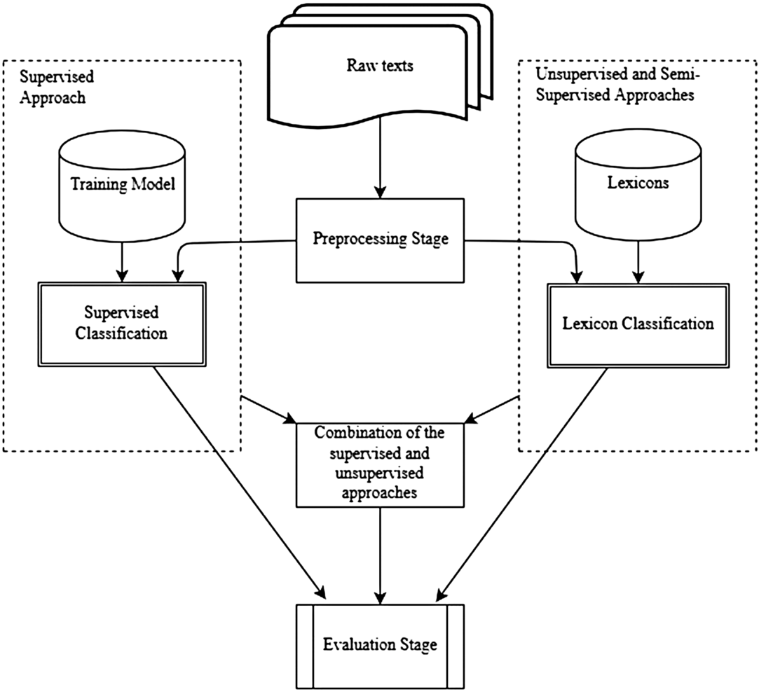
Figure 1. The flowchart of the proposed model.
3.1 Preprocessing and feature extraction
The features that we used in this study for the sentiment analysis of documents are as follows:
-
• Term frequency: The frequency of a word is an indicator about the importance of that word. As in several types of classification problems, this feature is widely used in the sentiment classification task. The frequency of a word is an indicator about the importance of that word. As a variation of term frequency, we used the tf-idf metric.
-
• POS tag: Some POS tags may carry more salient information than the other tags in sentiment analysis. For instance, adjectives are usually considered the key sentiment-bearing words. However, all the words with any POS tag can also be used. We employed both of these strategies in identifying the features. Different morphological analysis and disambiguation tools can be used in different languages to extract the POS tags of the words.
-
• Sentiment words and phrases: As mentioned, adjectives are good indicators for expressing opinions. Nevertheless, verbs, such as love, adverbs, such as fascinatingly, and out-of-vocabulary (OOV) words, such as 9/10, can also serve as features. In addition, phrases can be used to express sentiments (e.g., “cost someone an arm and a leg”). We, therefore, took all of them into account to evaluate how they contribute to the performance.
-
• Sentiment shifting: Negation words may cause the sentiment to change. For example, the sentence “I did not like it much” is of negative polarity, although it contains a positive sentiment word, which is like. But the use of this negation word (not) does not always imply that the sentiment has to shift, as in “I adored not only her elegance, but also her intelligence.” In this case, the sentiment word adore still has a positive meaning. We made use of the negation words and suffixes used in Turkish for sentiment shifting.
-
• Rules of opinions: Some rules may be applied while extracting sentiment features. For instance, if the word less or more is used, the sentiment word following it can be assigned a different score. Another one would be that if an entity consumes a resource in large quantities, as in “this washer uses up a lot of water,” it would be assigned a negative score, or if it rather contributes to the production, a positive score. We applied a set of intensifiers that cause a relative increase or decrease in the scores of the words.
Using all the words except those whose frequency is below a threshold value improved the performance. During the feature extraction stage, we applied the following preprocessing operations:
-
• While writing a text in Turkish, people sometimes prefer to use English characters for the corresponding Turkish characters, such as u (guzel) for ü (güzel (beautiful)). We use the Zemberek tool (Akın and Akın Reference Akın and Akın2007) to correct these characters.
-
• We do not remove emoticons, such as “:)” and “:(”, since they carry sentiment information. If the constituent characters of these emoticons are repeated, we normalize them such that this extra information is not lost (e.g., “:((((” is normalized as “:((”). In order to capture all of these kinds of emoticons, we use regular expressions.
-
• We remove all punctuation marks except “?”, “(!)”, and “!”, since they do not contribute to the sentiment expression. If a reviewer spells the exclamation mark(s) repeatedly in a sequence (e.g., “?!”), he/she most probably intends to express a negative sentiment. For instance, in the sentence “And you say that she is beautiful??!!,” it is apparent that the reviewer emphasizes a negative fact concerned with some entity (person).
-
• Similar to the repetition in punctuation marks, we assume that words with repeated characters (e.g., müthişşşş (greatttt)) are used for emphasis and we increase the score of such words. In addition, we assign a larger score to uppercased words. However, if all the words in a review are uppercased, we assume that there are no emphasized words, and there is no extra information to be exploited for sentiment classification.
-
• After performing these normalization processes, we also apply the İTÜ tool (Torunoğlu and Eryiğit Reference Torunoğlu and Eryiğit2014) to find other unnormalized tokens that the previous techniques could not detect.
-
• We then feed the words as input into the morphological parsing Sak, Güngör, and Saraçlar (Reference Sak, Güngör and Saraçlar2008) and disambiguation Sak, Güngör, and Saraçlar (Reference Sak, Güngör and Saraçlar2007) tools and obtain the morphological analysis of each word. In the methods that we use in this work, we consider three cases for the words: root form, surface form, and partial surface form (Section 3.2). Since Turkish is an agglutinative language and has a rich morphological structure, it is possible that the removal of suffixes may hamper the performance. The use of three different schemes enables us to observe the effect of suffixes in sentiment analysis.
Apart from these operations, we perform intensification, negation handling, and stop word elimination while determining the features. In Turkish, words can be negated as follows:
-
• The word değil (not) shifts the sentiment/semantic orientation of the word it follows. For instance, in “hoş değil bu şarkı” (this song is not nice), the positive word hoş (nice) is negated.
-
• Some verbal morphemes in Turkish (e.g., ma/me) switch the semantic orientation of the verbs. For example, sevdim (I liked) is of positive polarity, whereas sevmedim (I did not like) has a negative orientation.
-
• The word yok (there is not) makes the word it follows “absent.” For instance, in the sentence “umut yok artık” (there is no hope anymore), the word umut (hope) has no effect after it is followed by yok.
-
• Another case for negation is the use of the morphemes sız, siz, suz, and süz. For example, umutsuz (hopeless) has a negated meaning.
The morphological parser and disambiguation tools we utilize detect whether or not a word has a negation morpheme. When a negation morpheme or word is detected, we add an underscore at the end of the root of the negated word. For example, if the word is sevmedim (I did not love), the feature would be defined as sev_. In the case that negation morphemes/words occur consecutively, the negation effect is removed. For example, in the sentence “tatsız değil” (it is not tasteless), one negation morpheme and one negation word come one after another, so the statement loses its negative form. Therefore, we do not negate the token tat (taste) in this case.
In the stop word elimination phase, we exclude some words that function as stop words in general domain, but that have a sentiment-bearing role in sentiment analysis. For instance, the words çok (very) and bayağı (quite) intensify the polarity scores of the words following them. In this case, the intensifying word is eliminated, but the score of the word it modifies is increased. If there are repeating occurrences of these intensifiers, as in “çok çok güzel” (“very very beautiful”), the score of the word they intensify increases even more. Also, some words contribute to the intensification process more than others. For instance, the word daha (more) modifies the meaning of the following word less than the word en (most). Therefore, we assign different scores to these modifiers, which are to be used in the classification stage.
The range of polarity scores of the words is
 $(\!-\infty, \infty)$
. The polarity of a word is multiplied by
$(\!-\infty, \infty)$
. The polarity of a word is multiplied by
 $-1$
when negation occurs. In the case of double negation, the score does not change. We divided the intensifiers into several groups. For the intensifier “more” and its equivalents (“very,” “quite,” etc.), we multiply the score of the related word by 1.2. On the other hand, in case the modifier words “less” and its equivalents (“so so,” “a little,” etc.) occur in the text, we multiply the score of the affected word by 0.8. If a sequence of intensifiers occurs, the multiplicative factor becomes
$-1$
when negation occurs. In the case of double negation, the score does not change. We divided the intensifiers into several groups. For the intensifier “more” and its equivalents (“very,” “quite,” etc.), we multiply the score of the related word by 1.2. On the other hand, in case the modifier words “less” and its equivalents (“so so,” “a little,” etc.) occur in the text, we multiply the score of the affected word by 0.8. If a sequence of intensifiers occurs, the multiplicative factor becomes
 $1.2^{x}$
for the strengthening modifiers and
$1.2^{x}$
for the strengthening modifiers and
 $0.8^{x}$
for the weakening modifiers, where x is the number of intensifiers appearing consecutively. For the other intensifier, “most,” the score of the word is multiplied by 1.5, and for “least,” it is multiplied by 0.5. The weight parameters were determined empirically by observing their effects on the two corpora.
$0.8^{x}$
for the weakening modifiers, where x is the number of intensifiers appearing consecutively. For the other intensifier, “most,” the score of the word is multiplied by 1.5, and for “least,” it is multiplied by 0.5. The weight parameters were determined empirically by observing their effects on the two corpora.
We aim to build sentiment analysis models in this work that can be applied both to datasets with standard spelling (e.g., movie reviews) and also to datasets with a different jargon (e.g., Twitter). We eliminate words occurring less than a threshold (we use 20 as the threshold for the movie dataset and 5 for the Twitter dataset) to decrease the noise. In order to be able to cover the Twitter case, we tweak the normalization process further. We eliminate uniform resource locators (URL), since these kinds of tokens do not contribute to the sentimental meaning of a tweet. However, we keep the hashtags in the tweets since hashtags were reported to contribute to the sentiment (Davidov, Tsur, and Rappoport Reference Davidov, Tsur and Rappoport2010). This was also supported by our preliminary experiments. The preprocessing steps on an example tweet are shown in Table 2. In this example, the roots of the words are used.
Table 2. A sample tweet and effect of each preprocessing operation in the pipeline

In addition to using unigrams (tokens) only as features, we also utilize patterns and multiword expressions (MWEs) which are formed of word n-grams (for
 $n > 1$
). We make use of the TDK (Türk Dil Kurumu—Turkish Language Institution) dictionary to extract MWEs, such as idioms. A multiword term may have an effect on the sentiment that cannot be observed by the constituent words. For instance, the idiom “nalları dikmek” (to kick the bucket, literally “to raise the horseshoes up in the air”) has a negative sentimental meaning, whereas its constituent words are mostly neutral. Patterns are obtained as bigrams, where the consecutive two words conform to a set of rules based on the POS tags, as in Turney (Reference Turney2002). For example, the pattern rule “adverb+adjective” extracts each occurrence of an adverb followed by an adjective as a bigram feature. As will be seen in Section 4.3, while the use of MWEs in addition to the unigram features contributes to the performance of the classifier, this is not the case for patterns.
$n > 1$
). We make use of the TDK (Türk Dil Kurumu—Turkish Language Institution) dictionary to extract MWEs, such as idioms. A multiword term may have an effect on the sentiment that cannot be observed by the constituent words. For instance, the idiom “nalları dikmek” (to kick the bucket, literally “to raise the horseshoes up in the air”) has a negative sentimental meaning, whereas its constituent words are mostly neutral. Patterns are obtained as bigrams, where the consecutive two words conform to a set of rules based on the POS tags, as in Turney (Reference Turney2002). For example, the pattern rule “adverb+adjective” extracts each occurrence of an adverb followed by an adjective as a bigram feature. As will be seen in Section 4.3, while the use of MWEs in addition to the unigram features contributes to the performance of the classifier, this is not the case for patterns.
3.2 Additional preprocessing step: partial surface forms
The morphologically rich structure of Turkish makes it possible to extract and use some additional features in classification tasks. In most of the studies, either the root forms or the surface forms of the words are used (Yıldırım et al. Reference Yıldırım, Çetin, Eryiğit and Temel2014). However, in the domain of sentiment classification, some morphemes carry more sentimental information than the others. For instance, the suffix -cağız as in “kızcağız” (poor girl) denotes a sentiment of pity. As another example, conditional morphemes in Turkish, such as -se/-sa as in “keşke çalışsa” (I wish he/she worked), are indicative of expressing wishes or sentiments indirectly. Therefore, in this work, we take account of these morphemes while building the feature set, in addition to using the surface and root forms of the words as features. In our datasets, we have a set of 114 distinct morpheme tags.
We use an approach formed of two steps. In the first step, we compute the polarity scores of all the words in surface form using the delta tf-idf metric (see Equation (7)). Then, we parse and disambiguate the words using the morphological tools (Sak et al. Reference Sak, Güngör and Saraçlar2007; Sak et al. Reference Sak, Güngör and Saraçlar2008) to extract the morphemes. By assuming that a morpheme in a word has the same polarity score as that word, the polarity score of each morpheme is computed by taking the average of the scores of the words in which it is used. For instance, if the morpheme -se/-sa occurs in two words in the corpus, whose surface forms are sevse (I wish he/she liked) and izlese (I wish he/she watched), the polarity score of the morpheme -se/-sa is computed as the average score of the delta tf-idf scores of these two words. We then choose a percentage of the morphemes with the highest confidence scores. While selecting the morphemes, we take into account the following issues:
-
1. Negation morphemes: Regardless of their polarity scores, we do not eliminate the negation morphemes. These morphemes have a significant role in later processing where they cause a shift on the sentiments.
-
2. Type and number of discriminating morphemes: When forming the set of discriminating morphemes, we include the same number of positive morphemes and negative morphemes. We observed that if the morphemes are selected based on their absolute scores without taking into account an equal sentiment distribution, the results are biased toward the polarity of the majority class. In the experiments, we also test with different percentages of top morphemes, ranging from 10% to 90% in increments of 10. This makes it possible comparing the amount of morpheme usage with root forms (no morphemes) and surface forms (all morphemes).
-
3. Root forms: We only remove morphemes with low discriminating scores. However, we do not remove the POS tags of root forms no matter what their delta tf-idf scores are. Its reason is that we perform a morphological analysis here and the roots of the words are independent of this process.
-
4. Using several corpora: During the training phase, the morpheme scores are computed using the training part of the dataset. In addition to this usual setting, we also analyze the effect of incorporating other corpora into the process. While working on sentiment analysis on a domain (dataset), we extract the morpheme scores using both the training part of this dataset and the entire dataset of the other domain. The score of a morpheme is computed as the average of its scores calculated separately on the two datasets. The process can be generalized to more than two datasets easily. As will be stated in the experiments, we observed that using additional information by the use of other domains provides generalization and prevents overfitting.
In the second step, after the morpheme polarity lexicon is built, all the words are processed again and the morphemes that are not in the set of the discriminating morphemes identified in the first step are stripped off the surface form. That is, we obtain a form of the word that is formed of the root and the discriminating morphemes, which we name as the partial surface form. For instance, if the morpheme -se/-sa has a high score, but the score of the possessive morpheme -m is below the threshold, then the word sevsem (I wish I liked) changes into sevse by removing the morpheme -m. In this way, the words sevsem and sevse (and possibly some other derived forms) are reduced to the same partial form. After the partial surface forms are obtained, they are used in the proposed methods as in the same way as the root forms and the surface forms. We observed in the experiments that the use of partial surface form yields better results than the surface form and the root form. The reason is that the partial form provides us with additional supervised information related to morphemes.
3.3 Unsupervised and semi-supervised approaches
Most of the studies carried out for sentiment analysis in Turkish use supervised techniques (e.g., Kulcu and Doğdu Reference Kulcu and Doğdu2016). These studies implement various feature selection and extraction methods. Despite the diversity of the supervised approaches, the only unsupervised approach for extracting sentiments in Turkish is the one that is based on translating the sentiment lexical databases into Turkish and performing further analyses (Vural et al. Reference Vural, Cambazoğlu, Şenkul and Tokgöz2012; Türkmenoğlu and Tantuğ Reference Türkmenoğlu and Tantuğ2014). Translating sentiment lexicons has three main drawbacks:
-
1. It is a laborious task in terms of human effort, and it is also error-prone.
-
2. A word expressing positive sentiment in a language may not have the same effect in another language. For example, in various parts of Asia, people may use the word “smile” in the text for covering up embarrassment, humiliation, or shame, which is likely a negative sentiment. In Vietnam, this word is used as a substitute for “I’m sorry” or other behavioral expression patterns (Fontes Reference Fontes2009). Therefore, the word smile cannot be assigned the same sentiment direction and score in Vietnamese as in English, which is a subjective topic.
-
3. Apart from the cultural aspect, even people speaking the same language may translate words differently. Thus, a word can be labeled as having different sentiments by different translators.
Due to these drawbacks, instead of translating an available sentiment lexicon into Turkish, we develop methods that compute the sentiment strengths of the words automatically. We employ two algorithms, a domain-independent algorithm and a domain-specific algorithm, for this purpose. The first one obtains a general score for a given word without using any domain knowledge. We refer to this method as an unsupervised approach, since it does not make use of any sentiment information. We also build a domain-specific model to observe the effect of different domains on the polarity of some words. We call this a semi-supervised approach, since the seed words are determined using the domain and sentiment information. In the experiments (Section 4.3), we observed that the domain-specific approach outperforms the other approach, as can be expected.
3.3.1 Domain independent
In the domain-independent model, we generate the sentiment score (SC) of a word using the pointwise mutual information (PMI) scheme (Turney Reference Turney2002). Given a word word, the SC is computed as shown below:
 \begin{equation}\begin{aligned}SC(word) = \log_2\left(\frac{hits(word\ NEAR\ ``harika\textrm'{\textrm '})}{ hits(``harika{\text '}{\textrm'})} \times \frac{ hits(`berbat\textrm')}{hits(word\ NEAR\ ``berbat{\textrm'}{\textrm '})}\right)\end{aligned}\end{equation}
The words harika (great) and berbat (awful) form an antonym pair determined manually. NEAR is an operator that denotes, in the pattern “
 $w_1$
NEAR
$w_1$
NEAR
 $w_2$
,” the cooccurrence of the words
$w_2$
,” the cooccurrence of the words
 $w_1$
and
$w_1$
and
 $w_2$
. We use three different operators and patterns in this model as will be explained below. hits(query) returns the number of hits in a search engine given the query.
$w_2$
. We use three different operators and patterns in this model as will be explained below. hits(query) returns the number of hits in a search engine given the query.
Equation (1) is obtained by dividing the PMI formula for the pair word and harika (great) by the PMI formula for the pair word and berbat (awful) and then cancelling the hits(word) term in the denominator in the first one and the hits(word) term in the numerator in the second one. In this respect, we calculate the SC of the given word by taking the ratio of the frequency of its cooccurrence with a positive word (e.g., harika (great)) and the frequency of its cooccurrence with the corresponding negative word (e.g., berbat (awful)) and then normalizing with respect to the number of occurrences of this antonym pair. We perform smoothing by adding 0.001 to the hits function to prevent the case of zero occurrences. The higher the score of Equation (1) is, the more probable it expresses a positive sentiment; otherwise, a negative sentiment.
In contrast to other studies in Turkish, we get the hit frequencies from a search engine (YandexFootnote b), instead of using annotated corpora. We analyze the success of the search mechanism using one operator and two collocational patterns. The operator “
 $w_1$
NEAR(k)
$w_1$
NEAR(k)
 $w_2$
,” as stated above, returns the number of cooccurrences of the given words within a window of size k. The collocational patterns are “
$w_2$
,” as stated above, returns the number of cooccurrences of the given words within a window of size k. The collocational patterns are “
 $w_1$
ve
$w_1$
ve
 $w_2$
” (“
$w_2$
” (“
 $w_1$
and
$w_1$
and
 $w_2$
”), such as “akıllı ve güzel” (“smart and beautiful”), and “hem
$w_2$
”), such as “akıllı ve güzel” (“smart and beautiful”), and “hem
 $w_1$
hem
$w_1$
hem
 $w_2$
” (“both
$w_2$
” (“both
 $w_1$
and
$w_1$
and
 $w_2$
”), such as “hem cin fikirli hem çalışkan” (“both astute and hardworking”). We use these kinds of conjunctions as operators since they are used in connecting words, phrases, or clauses that have similar semantic or sentiment orientations. For example, it sounds more sensible to say “hardworking and beautiful” rather than “lazy and beautiful”. That is, the conjunction “and” generally connects two words which are of the same polarity.
$w_2$
”), such as “hem cin fikirli hem çalışkan” (“both astute and hardworking”). We use these kinds of conjunctions as operators since they are used in connecting words, phrases, or clauses that have similar semantic or sentiment orientations. For example, it sounds more sensible to say “hardworking and beautiful” rather than “lazy and beautiful”. That is, the conjunction “and” generally connects two words which are of the same polarity.
We observed that the NEAR operator returns more hits and gives rise to better sentiment scores compared to the collocational patterns. We tried out several values for the window size and found the optimal window size as
 $k = 12$
for the NEAR operator. The optimal value was determined by observing the final performance of the sentiment classifier with word polarity scores obtained with each window size. When k is increased more, expressions with different sentiments tend to occur more. On the other hand, choosing a small window size misses the cooccurrences of the collocated words.
$k = 12$
for the NEAR operator. The optimal value was determined by observing the final performance of the sentiment classifier with word polarity scores obtained with each window size. When k is increased more, expressions with different sentiments tend to occur more. On the other hand, choosing a small window size misses the cooccurrences of the collocated words.
We have manually chosen 10 antonym pairs from most commonly occurring nonstop words, as shown in the first part of Table 3. We decided to use 10 antonym pairs as seed words in accordance with the studies in the literature (e.g., Dehkhargani et al. Reference Dehkhargani, Saygn, Yanıkoğlu and Oflazer2016). The size of the seed set may seem small. However, using antonym words that are most likely indicative of popular and strong sentiments may capture the inherent polarities of corpus words accurately.

Table 3. Sets of sentimentally antonym pairs chosen manually for the domain independent and the domain-specific approaches

We compute the polarity score of a given word using Equation (1) with respect to each antonym pair and take the average. The reason of using 10 different pairs and their average, instead of a single word pair, is to prevent the bias that could occur toward that single pair. The overall score of a document (review) is obtained by summing the sentiment scores of the words it includes. If the score is greater than zero, it is predicted as a positive review, otherwise as a negative review. We considered only the words with POS label noun, adjective, verb, and adverb in the reviews. We observed in the preliminary experiments that other words, such as conjunctions, do not generally contribute to the overall sentiment expression of the review. This unsupervised approach is summarized in Algorithm 1.
3.3.2 Domain specific
The method given in the previous section assigns a polarity score to a word without taking the domain of the document into account. However, the polarity direction and score of a word may be different in different contexts. For instance, the word “unpredictable’’ expresses a positive sentiment in the movie domain (“unpredictable plot”), whereas it expresses a negative sentiment in car reviews (“unpredictable steering”). To take this into account and to build a domain-specific model, in this work, we have adapted the work of Hamilton et al. (Reference Hamilton, Clark, Leskovec and Jurafsky2016) to Turkish with minor changes. We applied the method to the movie domain and the Twitter dataset, but it can be applied to different domains with slight modifications. In the rest of this section, we explain the method for the movie domain.
As in the domain-independent approach, we choose manually a set of positive and negative word pairs. In this case, however, the words are specific to the movie domain. The list of the antonym word pairs is shown in the second part of Table 3. As can be seen in the table, the seed word sets in the domain-independent and domain-specific cases can overlap. This indicates that some words, such as “güzel” (beautiful) and “çirkin” (ugly), can be considered as generic and specific to a domain at the same time.
Based on the seed words determined manually, we use a propagation algorithm in order to induce a sentiment lexicon for that domain. The idea underlying the algorithm is that two words have similar sentimental meanings if they cooccur frequently or (even if they do not cooccur many times) if their contexts are “similar.” We construct a graph whose nodes correspond to words. Words are connected to each other via links that represent how often they cooccur. The higher the weight of a link is, the closer the two words is.
In order to compute the edge weights, we first build a matrix M which holds the PPMI (positive PMI) scores between all the words in the corpus. For two words
 $w_i$
and
$w_i$
and
 $w_j$
, the value of the matrix entry
$w_j$
, the value of the matrix entry
 $\textbf{M}_{i,j}$
is as follows:
$\textbf{M}_{i,j}$
is as follows:
 \begin{equation} \textbf{M}_{i,j} = {\rm ramp}\left(\log\left(\frac{p(w_{i}, w_{j})}{p(w_{i}) \times p(w_{j})}\right)\right)\\\end{equation}
Here, p(w) denotes the probability of the word w in the corpus, and
 $p(w_i,w_j)$
denotes the probability of cooccurrence of these two words within a sliding window of size 15. We tried out several values for the window size, which are 10, 15, 20, and 30. The highest success rates were obtained with window size 15. Since the cooccurrence statistics below zero do not make sense, the ramp function converts the negative values to zero. As the matrix is generated, we obtain a vector for each word w, which corresponds to the row for the word w in the matrix. Then the edge weights in the graph are calculated. If we denote the edge matrix as E, then the edge weight
$p(w_i,w_j)$
denotes the probability of cooccurrence of these two words within a sliding window of size 15. We tried out several values for the window size, which are 10, 15, 20, and 30. The highest success rates were obtained with window size 15. Since the cooccurrence statistics below zero do not make sense, the ramp function converts the negative values to zero. As the matrix is generated, we obtain a vector for each word w, which corresponds to the row for the word w in the matrix. Then the edge weights in the graph are calculated. If we denote the edge matrix as E, then the edge weight
 $\textbf{E}_{i,j}$
between two words
$\textbf{E}_{i,j}$
between two words
 $w_i$
and
$w_i$
and
 $w_j$
is simply the cosine similarity between the corresponding word vectors.
$w_j$
is simply the cosine similarity between the corresponding word vectors.
As the graph is built, we employ a random walk algorithm to propagate the edge weights within the graph and to calculate the sentiment scores of the words by taking into account both the cooccurrences and the seed words. Let v denote the vocabulary (set of words) in the graph (in the corpus). The method explained below is performed to find the positive polarities and the negative polarities of the words separately. Let
 $\textbf{P}_P$
and
$\textbf{P}_P$
and
 $\textbf{P}_N$
denote the vectors of, respectively, positive and negative polarity scores of the words. An entry in
$\textbf{P}_N$
denote the vectors of, respectively, positive and negative polarity scores of the words. An entry in
 $\textbf{P}_P$
(in
$\textbf{P}_P$
(in
 $\textbf{P}_N$
) corresponds to the positive (negative) polarity score of the corresponding word in v. We begin with
$\textbf{P}_N$
) corresponds to the positive (negative) polarity score of the corresponding word in v. We begin with
 ${\textbf{P}_P}^{(0)}$
and
${\textbf{P}_P}^{(0)}$
and
 ${\textbf{P}_N}^{(0)}$
that represent the initial vectors; each entry in
${\textbf{P}_N}^{(0)}$
that represent the initial vectors; each entry in
 ${\textbf{P}_P}^{(0)}$
and
${\textbf{P}_P}^{(0)}$
and
 ${\textbf{P}_N}^{(0)}$
is initialized with the value
${\textbf{P}_N}^{(0)}$
is initialized with the value
 $\frac{1}{|\textbf{v}|}$
. Then, we iteratively update the polarity score vector as follows (we explain the process for the positive polarity vector only; the case for negative polarities is analogous):
$\frac{1}{|\textbf{v}|}$
. Then, we iteratively update the polarity score vector as follows (we explain the process for the positive polarity vector only; the case for negative polarities is analogous):
 \begin{equation} {\textbf{P}_P}^{(k+1)} = (1 - g) \textbf{E} {\textbf{P}_P}^{(k)} + g \textbf{s}\end{equation}
In this equation, k denotes the iteration number. s is a (fixed) vector used for the positive seed words, where the positive seed words are assigned a weight of
 $\frac{1}{|\textbf{s}|}$
and the other words are assigned zero. In this respect, the equation is formed of two components. The matrix E incorporates cooccurrence information, and the vector s is used to bias toward the positive seed words. The contribution of each component is determined by a predefined constant g. Lower values of g favor the propagation of local information (cooccurrence values between neighbor nodes) via the E matrix, whereas higher values of g favor the global information (i.e., the positive seed values) via the s vector.
$\frac{1}{|\textbf{s}|}$
and the other words are assigned zero. In this respect, the equation is formed of two components. The matrix E incorporates cooccurrence information, and the vector s is used to bias toward the positive seed words. The contribution of each component is determined by a predefined constant g. Lower values of g favor the propagation of local information (cooccurrence values between neighbor nodes) via the E matrix, whereas higher values of g favor the global information (i.e., the positive seed values) via the s vector.
As the propagation within the graph continues, the scores of the words decrease at each iteration. This indicates that words close to the seed words may have similar scores to those of the seed words. However, words that are far away from the seed words are affected less by the propagation, thereby may have lower scores. To prevent this adverse effect, we steadily increase the local consistency score (i.e., decrease g), which is different than Hamilton et al. (Reference Hamilton, Clark, Leskovec and Jurafsky2016). The intuition behind it is that the seed words we chose may not be the optimal ones and may be misleading to some extent in determining the polarity scores of the words. We keep iterating the algorithm until convergence or a predefined maximum number of iterations (N) is reached.
Then, the positive polarity score vector
 $\textbf{P}_P$
is computed as follows:
$\textbf{P}_P$
is computed as follows:
 \begin{equation} \textbf{P}_P = \sum_{k=1}^{N} \frac{{\textbf{P}_P}^{(k)}}{k!}\end{equation}
Here, we take into account the vectors formed during the iterations, create a series, and take the sum of the series. At each step k of this sequence, we divide the score of that step by the factorial of k. We prefer the factorial function rather than the exponential decay or some other functions, since we want to weight the words close to the seed words more heavily. We observed in the experiments that using Equation (4) increased the performance by about 1% compared to the formulation in Hamilton et al. (Reference Hamilton, Clark, Leskovec and Jurafsky2016). By using a different formula from that work, we could observe the effect of different propagation coefficients. As stated above, we found out that words far away from the seed words should be weighed less heavily.
Finally, we form the polarity score vector denoted as P. For a word w, the entry in the polarity vector,
 $\textbf{P}(w)$
, is computed as shown in Equation (5).
$\textbf{P}(w)$
, is computed as shown in Equation (5).
 $\textbf{P}(w)$
being greater than zero indicates that the word has positive polarity, otherwise it has a negative polarity. We used a different formulation in Equation (5) than the one given in Hamilton et al. (Reference Hamilton, Clark, Leskovec and Jurafsky2016), and we observed a small increase in the success rates.
$\textbf{P}(w)$
being greater than zero indicates that the word has positive polarity, otherwise it has a negative polarity. We used a different formulation in Equation (5) than the one given in Hamilton et al. (Reference Hamilton, Clark, Leskovec and Jurafsky2016), and we observed a small increase in the success rates.
 \begin{equation} \textbf{P}(w) = \log\left(\frac{\textbf{P}_P(w)}{\textbf{P}_N(w)}\right)\end{equation}
After the word polarities are found, the score of a document is computed as the sum of the scores of words in the document, as in the domain-independent case. We again considered only the nouns, adjectives, verbs, and adverbs. Then the document is predicted as having positive sentiment if the score is greater than zero, and as having negative sentiment otherwise. For example, if the scores of the sentiment words in the sentence (review) given in Table 2 are “çok_güzel” [+3] and “:))” [+2], then the score of the sentence is +5 indicating that it is a review of positive polarity. The summary of the semi-supervised approach is given in Algorithm 2.

3.4 Supervised approaches
We divide the supervised approaches used in this work into two groups. The first one involves the use of classical machine learning algorithms. We developed several novel feature weighting schemes to be used in these methods. The second group consists of deep learning architectures. In this case, we employ much fewer preprocessing and feature extraction operations, since they are handled by these models implicitly.
3.4.1 Traditional machine learning methods and feature sets
In machine learning applications, the choice of the right features and feature values has a more important role on the success rates than the learning approach used. To this effect, we make use of different feature-weighting metrics. The first two are our variations of the delta idf and delta tf-idf metrics as shown in Equations (6) and (7), respectively (Martineau and Finin Reference Martineau and Finin2009). These two scoring metrics are state-of-the-art for the sentiment classification task since they utilize the sentiment and semantic orientation of the words in the training dataset. It outperforms the tf-idf metric as stated in the literature (Martineau and Finin Reference Martineau and Finin2009), as we also observed in this work.
 \begin{align} \text{delta idf$_{{w}}$} &=\log\frac{\frac{N_{P,w}}{N_P}+0.001}{\frac{N_{N,w}}{N_N}+0.001} \end{align}
 \begin{align} \text{delta tf-idf$_{{w,d}}$} &=\left(0.5 + 0.5 \times \frac{f_{w,d}}{{\rm max}_{\{w' \in d\}}\,f_{w',d}}\right) \times \text{delta idf$_{{w}}$}\end{align}
In Equation (6), delta idf
 $_{{w}}$
is the sentiment score of the word w in the corpus.
$_{{w}}$
is the sentiment score of the word w in the corpus.
 $N_P$
and
$N_P$
and
 $N_N$
correspond to the number of reviews, respectively, in the positive corpus (i.e., the corpus of positive documents) and in the negative corpus (i.e., the corpus of negative documents).
$N_N$
correspond to the number of reviews, respectively, in the positive corpus (i.e., the corpus of positive documents) and in the negative corpus (i.e., the corpus of negative documents).
 $N_{P,w}$
and
$N_{P,w}$
and
 $N_{N,w}$
denote the number of reviews in, respectively, the positive corpus and the negative corpus in which the word w occurs. Both the numerator and the denominator are normalized (divided by
$N_{N,w}$
denote the number of reviews in, respectively, the positive corpus and the negative corpus in which the word w occurs. Both the numerator and the denominator are normalized (divided by
 $N_P$
and
$N_P$
and
 $N_N$
) in order to overcome the imbalance problem between the two classes. We add 0.001 for smoothing. In the machine learning algorithms, the SC delta idf
$N_N$
) in order to overcome the imbalance problem between the two classes. We add 0.001 for smoothing. In the machine learning algorithms, the SC delta idf
 $_{{w}}$
is used as the weight of the word (feature) w, independent of the review.
$_{{w}}$
is used as the weight of the word (feature) w, independent of the review.
Equation (7) uses a variation of the tf-idf metric.
 $f_{w,d}$
denotes the frequency of the word w in document d. We divide this frequency by the frequency of the most frequently occurring word in the document d, denoted by
$f_{w,d}$
denotes the frequency of the word w in document d. We divide this frequency by the frequency of the most frequently occurring word in the document d, denoted by
 ${\rm max}_{\{w' \in d\}}\,f_{w',d}$
, to prevent a bias toward longer documents. delta tf-idf
${\rm max}_{\{w' \in d\}}\,f_{w',d}$
, to prevent a bias toward longer documents. delta tf-idf
 $_{{w,d}}$
is used in the learning phase as the weight of the word (feature) w in document d.
$_{{w,d}}$
is used in the learning phase as the weight of the word (feature) w in document d.
The third weighting scheme we use is the classical tf-idf metric. The difference from the previous two is that, in this case, we do not make use of the labels of the documents. That is, we compute a tf-idf value for each word in the whole corpus (of both sentiments) and use this value as the feature weight. The next method is using only three features for each review, which are the maximum, minimum, and mean polarity scores computed by Equation (7). As will be seen in Section 4.3, taking into account only these three features proves to be as useful as using the sentiment scores of all the words in a review. As a final scheme, we combine the tf-idf metric with the three-feature scheme. That is, these three features are added to the set of word features with tf-idf scores.
After the feature sets are obtained, we used several classifiers to test the performance. The machine learning algorithms we used are decision tree (J-48), SVM, NB, and k-nearest neighbor (kNN). The literature states that discriminative models generally outperform generative models in sentiment classification (Ng and Jordan Reference Ng and Jordan2002). We also observed this claim to be true, as will be shown in Section 4.3.
Besides the machine learning algorithms, we also implement a simple supervised method, which we name as log scoring (LS). Here, we simply sum the delta tf-idf scores of all the words in a review. If the sum is greater than zero, the review is predicted as positive; otherwise, it is predicted as negative. As will be seen, the performance of this method is nearly as high as the performance of the SVM classifier and it outperforms the kNN method.
3.4.2 Neural network methods
Apart from the classical machine learning approaches, we also used two state-of-the-art neural network architectures, which are the LSTM and convolutional neural network (CNN) models. For these models, we perform only tokenization in the preprocessing stage and do not deal with feature extraction. The reason is that these models are mostly capable of identifying the suitable features.
LSTM is a recurrent neural network (RNN) model composed of LSTM units (Hochreiter and Schmidhuber Reference Hochreiter and Schmidhuber1997). Each cell in this network “remembers” values over arbitrary time intervals and accounts for memory in the model. The three gates in these cells can be considered as conventional artificial neurons. An activation function is applied on the weighted sum of the outputs in these gates. This model is superior to conventional RNNs in the sense that the cells can remember the previous values more efficiently in a long-term dependency manner.
In the LSTM model we build, we perform classification on a review basis. We feed the word embedding vectors as input into the network. The word embeddings were trained on a large corpus of 951M words (Yıldız et al. Reference Yıldız, Tırkaz, Şahin, Eren and Sönmez2016) using the skip-gram model. A shallow model as in Mikolov et al. (Reference Mikolov, Chen, Corrado and Dean2013) is built to generate word embeddings, using a log-linear classifier. Words are predicted within a certain range before and after the target word. Since distant words are in general less related to the target word, their weights are decreased. The dimension of the word vectors is set to 300. The number of LSTM units is 196. We use a dropout rate of 0.4 to prevent overfitting. Dropout is enabled during training only, and it is disabled while evaluating the model. We use softmax as the activation function, since it is the most common activation function used for categorical cross-entropy problems like sentiment analysis. We set the maximum number of epochs to 200. As an early stopping criterion, if the error in the validation set starts to increase, we stop the training phase.
CNNs have recently gained importance mostly in the fields of image and video recognition, and also in natural language processing studies (Goldberg Reference Goldberg and Hirst2017). In classical feature selection, using fixed n-grams as features may cause loss of information. For instance, two trigram features whose first two words are the same but that differ in the last word are treated as different features. However, CNN overcomes this problem. Local aspects that are considered most informative for the prediction task at hand are captured.
We used an open-source CNN framework (Britz Reference Britz2017). We modified the code slightly to adapt it to Turkish and to utilize word vectors. We set the character encoding as UTF-8 in the code and removed some tokenization rules, which are specific to English. We added a few lines of code to feed static word embeddings into the model.
Then, convolutions are performed using multiple filter sizes. That is, the word vector values in the sliding windows are convolved to a single value. We employ max-pooling such that the most important feature for each filter is extracted. Dropout regularization, L2 values (used in combatting the overfitting problem), and other parameters are fine-tuned employing a validation set, and, lastly, we perform classification using a fully connected softmax layer.
We use both nonstatic word embeddings that are learned during the training phase and static (pretrained) word embeddings (Güngör and Yıldız Reference Güngör and Yıldız2017) as input. We utilize the same word embeddings as in the LSTM model. The skip-gram model extracts more information than the continuous “bag of words” model when a large corpus is available. We use 300 as the dimension size of the pretrained vectors. The embedding representation suffers less from the data sparsity problem and it is in general more informative compared to the PMI approach given in Section 3.3. That is, the method of taking account of the cooccurrence statistics between two words is behind the potential of vectors generated by processing a large corpus and fine-tuning the parameters of a shallow neural network. The algorithms corresponding to the supervised approach are given in Algorithm 3.
3.5 Combination of unsupervised and supervised approaches
The last approach we use is the combination of the unsupervised and supervised methods. If the unsupervised and supervised polarity scores of a word have different signs (one positive, the other negative), we consider that word as ambiguous in terms of polarity and take into account only a fraction of the supervised score. Otherwise, we take the weighted average of the unsupervised and supervised scores, as follows:
 \begin{equation} combSC_{w} = \begin{cases} c_{s} \times supervised\_score(w), & \text{if}\ opposite\\&\ \ \ signs \\ c_{u} \times unsupervised\_score(w) + c_{s} \times supervised\_score(w), & \text{otherwise} \end{cases} \end{equation}
Here, the unsupervised score and the supervised score refer to the scores computed in, respectively, Equations (1) and (7). For the supervised case, we chose the delta tf-idf score (Equation (7)), rather than the other weighting metrics, since it yields successful results in the experiments.
 $c_u$
and
$c_u$
and
 $c_s$
denote the coefficients of the unsupervised and supervised scores, respectively, such that
$c_s$
denote the coefficients of the unsupervised and supervised scores, respectively, such that
 $c_u + c_s = 1$
. In order to determine the best values of the coefficients, we first split the dataset into training, development, and test partitions. Then we performed grid search on the development set using nested 10-fold cross-validation, by ranging the coefficients between 0.1 and 0.9 in increments of 0.1. We could also use a supervised regression approach for learning those values. However, our simple approach defining an array of coefficients by grid search was efficient and reliable. We found the optimal values as
$c_u + c_s = 1$
. In order to determine the best values of the coefficients, we first split the dataset into training, development, and test partitions. Then we performed grid search on the development set using nested 10-fold cross-validation, by ranging the coefficients between 0.1 and 0.9 in increments of 0.1. We could also use a supervised regression approach for learning those values. However, our simple approach defining an array of coefficients by grid search was efficient and reliable. We found the optimal values as
 $c_u = 0.3$
and
$c_u = 0.3$
and
 $c_s = 0.7$
for both datasets. This indicates that the supervised score is more reliable and informative about a word’s polarity, thus it contributes more to the overall score. However, the unsupervised weight also has an effect and ignoring it causes the performance to decrease. When the signs of the unsupervised and supervised polarity scores contradict, we use only the supervised polarity score multiplied by
$c_s = 0.7$
for both datasets. This indicates that the supervised score is more reliable and informative about a word’s polarity, thus it contributes more to the overall score. However, the unsupervised weight also has an effect and ignoring it causes the performance to decrease. When the signs of the unsupervised and supervised polarity scores contradict, we use only the supervised polarity score multiplied by
 $c_s$
and the unsupervised component is ignored. The reason is that the supervised score is more reliable; however, due to ambiguity, we lessen its impact. After the feature scores are calculated in a combined manner, we feed them into classical machine learning algorithms. As will be seen in Section 4, using the combined approach improves the performance in some cases, especially when we do not perform intensification and negation handling. We give the summary of this approach in Algorithm 4.
$c_s$
and the unsupervised component is ignored. The reason is that the supervised score is more reliable; however, due to ambiguity, we lessen its impact. After the feature scores are calculated in a combined manner, we feed them into classical machine learning algorithms. As will be seen in Section 4, using the combined approach improves the performance in some cases, especially when we do not perform intensification and negation handling. We give the summary of this approach in Algorithm 4.


4. Experimental evaluation
We evaluated the proposed methods on raw text data in two domains for the binary sentiment classification problem in Turkish at document level. In order to test whether our approaches are portable to other languages, we evaluated the methods on two English datasets as well. In this section, we first give the details of the datasets and the values used for the hyperparameters. This is followed by the explanation of the experiments and comments on the results obtained.
4.1 Datasets
In this work, we used two datasets. The first one is a movie dataset composed of movie reviews in Turkish collected from a popular website.Footnote c This is the same dataset utilized in the work that we consider as baseline for comparison (Türkmenoğlu and Tantuğ Reference Türkmenoğlu and Tantuğ2014). The size of the dataset is 20,244 reviews, where the average number of words per review is 39. The reviews have star scores ranging from 0.5 to 5 in increments of 0.5 points. If the score of a review is equal to or lower than 2.5, it is considered as negative, whereas if the score is equal to or higher than 4, it is considered as positive. Accordingly, there are 13,224 positive reviews and 7020 negative reviews in this corpus.
The second dataset is a Twitter dataset formed of tweets in Turkish. The tweets in this corpus are much shorter and noisier compared to the reviews in the movie dataset. The training set is composed of 3000 tweets and was taken from the website of the Kemik NLP group of Yıldız Technical University. Tweets in this set are about two pioneering Turkish mobile network operators, Turkcell and Avea. The tweets in the development and test sets which cover various topics were collected by two undergraduate students and were annotated as positive, negative, and neutral. We removed the neutral reviews from the dataset since we perform binary sentiment classification. We merged all the sets, shuffled them, and applied 10-fold cross-validation. We thereby take into account several topics and domains in the same corpus and test how it affects the performance. There are 1716 tweets in total, where 743 of them are positive and 973 are negative. We measured the Cohen’s Kappa inter-annotator agreement score as 0.82.
We also employed three other datasets in English to test the portability of our approaches across languages. One of them is a movie corpus collected from the web (Pang and Lee Reference Pang and Lee2005). There are 5331 positive reviews and 5331 negative reviews in this dataset. The other is a Twitter dataset containing nearly 1.6 million tweets annotated through a distant supervised method (Go, Bhayani, and Lei Reference Go, Bhayani and Huang2009). In the method used, if a tweet includes a positive emoticon, it is labeled as positive and if it includes a negative emoticon it is labeled as negative. Otherwise, it is labeled as neutral. These tweets have positive, neutral, and negative labels. We have chosen 7020 positive tweets and 7020 negative tweets randomly. As a third dataset, we used the dataset collected for the SemEval 2017 competition (Rosenthal, Farra, and Nakov Reference Rosenthal, Farra and Nakov2017) to compare our performance against the contestants. Since we perform binary sentiment analysis, we chose the Subtask B dataset for “tweet classification according to a two-point scale.” This is formed of tweets including topic information along with sentiment. The training dataset consists of 20,508 tweets, whereas the test dataset is composed of 6185 tweets. We removed neutral and “off topic” reviews from the training set and processed the remaining 18,962 tweets.
Since we are given separate training and test datasets for the SemEval task, we have not performed cross-validation for this dataset. We utilized 20% of the training dataset as validation set to find the optimal values for the combination of supervised and unsupervised approaches. In the other datasets, for the approach combining the supervised and unsupervised methods, we used nested 10-fold cross-validation. In all the other experiments, we employed non-nested 10-fold cross-validation. We split the data into three parts: as 80% for training set, 10% for development set, and 10% for test set. The validation portion is used to determine whether the convergence criterion is met and to prevent overfitting.
4.2 Hyperparameters
We used the scikit-learn framework (Pedregosa et al. Reference Pedregosa, Varoquaux, Gramfort, Michel, Thirion, Grisel, Blondel, Prettenhofer, Weiss, Dubourg, Vanderplas, Passos, Cournapeau, Brucher, Perrot and Duchesnay2011) for the machine learning algorithms (J-48, SVM, kNN, and NB). In SVM, we used linear kernel since sentiment analysis is mostly considered as a linearly classifiable problem. For kNN, we chose k as three and used the cosine similarity metric. We chose k as an odd number to prevent ties while classifying a document. We label a review as positive or negative depending on the majority of the sentiments of its nearest neighbors.
For the LSTM network, we applied only tokenization in the preprocessing stage, since the model carries out most of the feature selection and extraction tasks inherently. In the case of CNN, we chose the number of filters as 128 and set the filter sizes as 3, 4, and 5. In this network, there are four layers, which are the word embedding layer, convolutional layer, max-pooling layer, and softmax layer. We chose the dropout rate as 0.5 and set the L2 regularization value at 0.005. We did not perform negation handling and multiword expression extraction, since the model is assumed to achieve this effect via the sliding windows. We have trained the network until the convergence criterion is met or for at most 200 epochs, similar to the LSTM case. If the loss on the validation set stopped decreasing, we consider the early stopping criterion is met.
4.3 Results
We first give the performances (F1-score) of the five feature weighting schemes in Table 4. Each metric was applied to both datasets using the classical machine learning methods. We should note that in this experiment we do not measure the success of a metric on a word basis. That is, we are not interested in how accurately a metric (say delta idf
 $_{{w}}$
) determines the polarity of a word. Instead, we measure the success on a review basis by using the polarity scores of the words in the review determined by the metric, and then classifying the review.
$_{{w}}$
) determines the polarity of a word. Instead, we measure the success on a review basis by using the polarity scores of the words in the review determined by the metric, and then classifying the review.
Table 4. Contribution of each weighting scheme to the performances (%) of the supervised approaches for the two datasets

In the experiments, we tested the methods using the surface forms of the words, the root forms of the words, and the forms obtained by concatenating the roots with the morphemes having the highest confidence scores (partial surface forms). We found that using the partial surface forms of words as features yields the best results. Another observation is that, unlike the unsupervised and semi-supervised approaches, using all the tokens gives better success rates than using only words of some specific POS tags (e.g., noun, adjective, verb, adverb). The intuition behind it is that some tokens that are not morphologically correct words (e.g., the token 10/10 in a movie review) may carry sentimental information. The figures in Table 4 correspond to partial surface form and all tokens cases.
Table 5. Summary of performances (%) of the unsupervised, semi-supervised, and supervised methods (using the 3 feats technique), and their combinations for the two datasets

We see that the best success rates were achieved using the 3 feats model for both datasets, which is a simple model that uses only three features. This is an interesting result. This result can be attributed to the specific nature of the sentiment classification problem. In this problem, the average sentimental meaning of a document accompanied with the maximum and minimum word values may successfully signal the sentiment of the document. That is, it takes into account the most extreme values occurring in a review. If the maximum, minimum, and mean polarity scores of a review differ from each other to a great extent, we would say that it has “borderline” traits. This is similar to how extreme values are captured in the pooling operation of CNNs. For example, the first reviewer may say “Graphics were hilarious; the plot was OK. However, the actress was beyond terrible.” On the other hand, the second commentator’s review could be “All the graphics, plot, and actors were OK.” Although the two reviews might have the same mean polarity score, the variance occurring in the first review is much wider. That is, it can be considered an outlier review, affecting the performance in a different manner.
Table 5 shows the results of the unsupervised (Section 3.3.1) and semi-supervised (Section 3.3.2) approaches, compares them with the supervised case, and also shows the effect of various combination strategies on the success rates. For the supervised case, we include the results of the 3 feats method obtained with SVM, which are the most successful results. All the experiments were conducted with both the combination of unigrams and MWEs, and patterns. We see that the use of patterns results in worse performance. The unsupervised and semi-supervised success rates are much lower than those of the supervised learning approaches. We tested several combinations of the four supervised methods using majority voting. The combination of J-48, SVM, and NB achieved the highest results. The results obtained under this ensemble of classifiers outperformed SVM with a small margin. This result indicates that in some cases the instances misclassified by a classifier are compensated by the other classifiers. The final result we obtained is the combination of the unsupervised and supervised methods (Section 3.5). This combination using the majority voting scheme yields the highest performances. Its being even higher than the ensemble of classifiers signals the necessity of the unsupervised metric in sentiment classification. The result obtained on the movie domain (91.17%) outperforms the baseline study in Turkish (Türkmenoğlu and Tantuğ Reference Türkmenoğlu and Tantuğ2014) by a significant margin, in which an accuracy of 89.5% was obtained on the same dataset. Our success rate is also the highest for the binary sentiment classification task in Turkish on the movie dataset, to the best of our knowledge.
Although the neural network architectures we used are supervised models, we show them separately from the classical supervised models, since they are not subjected to different feature weighting schemes as in Table 4. Table 6 shows the performances of the deep learning models. Using static word vectors (word2vec) results in worse performance compared to the nonstatic word vectors. The reason is that in the nonstatic case we learn the embeddings during the training phase by taking into account the sentiment information. On the other hand, the static vectors are pretrained, and we do not use class labels to learn them. As in all other experiments, the use of word embeddings and neural models led to lower success rates for the Twitter dataset compared to the movie dataset. This can be attributed to the Twitter’s distinctive and noisy content, which makes it more difficult to normalize the tweets successfully. There are many OOV words that could not be normalised, so they lack their corresponding word embeddings. Since there are relatively less OOV words in the movie corpus, we could feed their available embeddings into the network and obtain better performance as compared to the Twitter dataset.
Table 6. Performances (%) for two neural network models using different word embedding types for the two datasets

An interesting point that we observed in the CNN experiments is that when we perform intensification and negation handling and take account of MWEs, the success rates drop by about 2%. Since the filtering mechanism within the framework carries out these tasks, our intervention proves to be not only unnecessary but also harmful. For example, when we perform negation handling (e.g., “güzel değil” (not beautiful) is converted to “güzel_” (beautiful_)), SVM generates better results, whereas CNN does not. Thus, some feature engineering techniques may have opposite effects on different machine learning algorithms.
In the literature, neural network models used in this work are in general reported to outperform classical learning methods. However, the success rates we obtained using the LSTM and CNN models are not as high as those produced by the supervised methods used, especially with the 3 feats feature set and the majority voting scheme. That is, we found out that conventional machine learning methods, by utilizing different feature engineering techniques, could perform better than the two popular neural network models. However, when we do not employ those feature selection methods, neural networks outperform the classical machine learning methods. We think that this is due to the advanced nature of the feature extraction processes used in the conventional methods. The neural models could not compensate for the advanced features by the deeper learning schemes. For instance, in the SVM approach, we made use of MWEs, whereas in the neural networks, word embeddings for those expressions and phrases were absent. Another case is that we can intensify the polarity strengths of words and feed these modified input vectors to the classical machine learning methods. However, we cannot intensify or modify the word embeddings’ values that are generated by Yıldız et al. (Reference Yıldız, Tırkaz, Şahin, Eren and Sönmez2016).
It can be argued that the performance of the neural models will improve if the OOV words are handled properly. There are several ways to decrease the number of OOV words and generate embeddings for such words in the literature (Chen and Yu Reference Chen and Yu2018; Garneau, Leboeuf, and Lamontagne Reference Garneau, Leboeuf and Lamontagne2018). For instance, the embedding of an OOV word can be taken as the average of the embeddings of its context words (Horn Reference Horn2017). The success rates of the neural models may increase if we include these words in the models. However, since most of the OOV words occur rarely and we remove the words that occur below a frequency threshold, this may result only in a slight increase in the performance. We leave a detailed analysis of this issue for future research.
We made a detailed analysis related to the use of partial surface forms on the Turkish datasets. We tested the effects of using different ratios of morphemes and training the morpheme polarity scores on several datasets and compared the results with those obtained using root forms and surface forms. The results are shown in Figure 2 (movie dataset) and Figure 3 (Twitter dataset). The results were obtained using the 3 feats metric and the SVM method. The horizontal axis in the figures denotes the ratio of morphemes with the highest confidence scores that are included in the partial forms. The ratios of 0% and 100% correspond, respectively, to the root form and the surface form. The partial surface form was experimented in two settings: using one corpus (training part of the dataset) and using two corpora (training part of the dataset and all parts of the other dataset). The figures show that when we use a subset of the morphemes by taking into account their discriminating power, we outperform the use of the root form and the surface form with nearly all ratios of the top morphemes. We attribute the success of the partial surface forms to several factors. Morphemes with absolute scores near zero are neutral and can be considered as noise, and they are better to be removed. By using the most informative morphemes based on their supervised scores, we enhance the sentiment representation for words in an agglutinative language. With respect to the use of several datasets in training the morpheme polarities, we observe that it especially contributes in the case of the Twitter domain (Figure 3) by incorporating an additional, less noisy dataset.

Figure 2. Effect of morphological analysis with respect to different top morpheme ratios on the Turkish movie dataset.
Table 7 summarizes the effect of different morphological forms on the performance. For the partial surface form, we include the best results given in Figures 2 and 3, which correspond to 90% of the morphemes for the movie dataset and 50% for the Twitter dataset. The best success rates are obtained using partial surface forms. We thus observe that using a number of discriminating morphemes is the most effective method for sentiment classification in Turkish. The results are significant at
 $P=0.05$
compared to both root form and surface form.
$P=0.05$
compared to both root form and surface form.
Table 7. Summary of the effects of morphological analyses on performances (%) for the two Turkish datasets using the SVM method and the 3-feats metric


Figure 3. Effect of morphological analysis with respect to different top morpheme ratios on the Turkish Twitter dataset.
We analyze the contribution of the preprocessing operations (Sections 3.1 and 3.2) on the success rates. We show the effect of each operation in Table 8. We use the delta tf-idf
 $_{{w,d}}$
metric and SVM. Normalization refers to the operations of deasciification, punctuation removal, and other normalizations by the İTÜ tool. Noise elimination is removal of tokens occurring less than seven times. In the MWE step, multiword terms are included in addition to the unigram features. The steps denoted by emoticons, negation handling, and intensification correspond to, respectively, including emoticons also in the feature set, processing negation words and suffixes, and taking intensifiers into account. In the partial surface forms step, we use partial forms formed of 90% and 50% of the top morphemes for the movie and Twitter datasets, respectively, trained on two corpora. As shown in the table, it increases the success rates with a significant margin for the movie dataset and with a small margin for the Twitter dataset. Finally, the all POS step refers to using all the words, instead of using only the four categories (noun, adjective, verb, adverb) as in the previous steps. We see that each step adds to the success rate. In the Twitter case, normalization and removing the POS restriction also boost the performance because of the idiosyncratic nature of the medium and the large number of OOV words. In summary, normalization, using partial surface forms, and using all the tokens regardless of their POS tags are found to be the most effective methods to increase the success rates.
$_{{w,d}}$
metric and SVM. Normalization refers to the operations of deasciification, punctuation removal, and other normalizations by the İTÜ tool. Noise elimination is removal of tokens occurring less than seven times. In the MWE step, multiword terms are included in addition to the unigram features. The steps denoted by emoticons, negation handling, and intensification correspond to, respectively, including emoticons also in the feature set, processing negation words and suffixes, and taking intensifiers into account. In the partial surface forms step, we use partial forms formed of 90% and 50% of the top morphemes for the movie and Twitter datasets, respectively, trained on two corpora. As shown in the table, it increases the success rates with a significant margin for the movie dataset and with a small margin for the Twitter dataset. Finally, the all POS step refers to using all the words, instead of using only the four categories (noun, adjective, verb, adverb) as in the previous steps. We see that each step adds to the success rate. In the Twitter case, normalization and removing the POS restriction also boost the performance because of the idiosyncratic nature of the medium and the large number of OOV words. In summary, normalization, using partial surface forms, and using all the tokens regardless of their POS tags are found to be the most effective methods to increase the success rates.
Table 8. Contributions of preprocessing modules to the performance (%) of the SVM method using the delta tf-idf metric

Table 9. Summary of performances (%) of the unsupervised, semi-supervised, and supervised methods and their combinations for the three datasets in English

As a final experiment, we also evaluated the proposed methods on three datasets in English in order to test the portability of the approaches across languages. To give an overview, we show the most important findings which are produced by a subset of the methods and the feature engineering techniques. We do not apply morphological operations on the words (negation suffixes, partial surface forms, etc.) since English has a simple morphological structure. The results are shown in Table 9. For the SemEval 2017 dataset, in addition to the F1-scores shown in the table, we also computed the “average recall” values as stated in the relevant paper in order to compare with other participants. In the “unsupervised + supervised majority voting” scheme, we obtained a score of 77.9% and ranked 15th among 24 teams, including us. For this scheme, we found the optimal coefficients to be 0.6 and 0.4 for the supervised and unsupervised components, respectively, utilizing the validation set. When we leverage other approaches, we rank worse overall. As in the case of Turkish, combining the unsupervised and supervised methods gives rise to the best success rates. When we compare the classical machine learning models and the neural models, we see that they have similar performances. We do not observe a large difference between the two paradigms as in Turkish, probably due to the simpler nature of the feature extraction process in this case.
The most similar work to ours carried out for sentiment analysis in Turkish is the work of Türkmenoğlu and Tantuğ (Reference Türkmenoğlu and Tantuğ2014). They employ unigram and bigram features with tf-idf weights and obtain an accuracy of 89.5% on the same movie dataset. We observed in our work that combining the supervised algorithms with unsupervised approaches leads to better performance. We used paired t-test and the approximate randomization technique to measure the significance of the difference between the two works. The result obtained with the combined method (91.17%) significantly outperforms the success rate obtained in Türkmenoğlu and Tantuğ (Reference Türkmenoğlu and Tantuğ2014) on the same dataset at
 $P=0.05$
. Kaya et al. (Reference Kaya, Fidan and Toroslu2012) also used several supervised machine learning methods in the domain of political news. They analyzed the effect of different types of features, such as unigrams and bigrams, adjectives, and a predefined list of sentiment words, with term frequency and boolean weights. They obtained an accuracy of 77%. To the best of our knowledge, employing a semi-supervised domain-specific approach, combining unsupervised and supervised approaches, utilizing the partial surface forms method, and making use of both static and nonstatic word embeddings in neural architectures for Turkish are the novel aspects in the proposed approaches.
$P=0.05$
. Kaya et al. (Reference Kaya, Fidan and Toroslu2012) also used several supervised machine learning methods in the domain of political news. They analyzed the effect of different types of features, such as unigrams and bigrams, adjectives, and a predefined list of sentiment words, with term frequency and boolean weights. They obtained an accuracy of 77%. To the best of our knowledge, employing a semi-supervised domain-specific approach, combining unsupervised and supervised approaches, utilizing the partial surface forms method, and making use of both static and nonstatic word embeddings in neural architectures for Turkish are the novel aspects in the proposed approaches.
5. Conclusion and future work
In this paper, we developed a framework for two-class sentiment classification problem in Turkish. The documents were first subjected to comprehensive preprocessing operations tailored for the language and then features were extracted based on the normalized texts. We proposed methods that follow three main approaches. In the unsupervised/semi-supervised approach, the polarity score of words was determined using a set of antonym seed words and then the sentiment of a document is obtained as the sum of the scores of the words it contains. In the supervised approach, we used several feature-weighting metrics including novel metrics. The supervised methods were analyzed in two groups, which are the classical learning algorithms and the deep learning models. Finally, the third approach formed ensembles of classifiers and also combined the unsupervised and supervised approaches.
We observed the performance of all these methods on two datasets with different characteristics. We conclude that combining unsupervised/semi-supervised and supervised methods yields the best results in both datasets. This indicates that incorporating knowledge obtained in an unsupervised manner into the classification process seems to be necessary to obtain more successful results. To the best of our knowledge, this is the first work in Turkish that extracts sentiment scores of words using search engines, that employs domain-specific sentiment analysis, and also that combines unsupervised and supervised schemes. The unsupervised and semi-supervised approaches can be adapted to other domains and languages easily by choosing a relevant set of antonym pairs.
The experiments have shown that the feature engineering techniques used in determining the features and using suitable weighting schemes are the most important aspects in the supervised case. We observed that some preprocessing operations and specific feature selection methods hamper the performance in some of the learning algorithms, such as negation handling and intensification in the CNN framework. Another observation is related to the agglutinative nature of the language in the sense that, in addition to the root forms of the words, making use of the morphemes within the surface forms gives rise to better results after performing normalization. We have also shown that conventional machine learning algorithms using novel and effective feature engineering techniques outperform the deep learning models.
Since Turkish has a rich morphological structure, using morphological features improved the performance. We observed that some morphemes are more indicative of the sentiment of words. The supervised approach we developed can be adapted to other morphologically rich languages without any manual effort to create morphological sets and high performances can be achieved as long as training data are available. Even if there is no training data in a language, the sentiment scores of morphemes can still be computed by employing unsupervised and semi-supervised approaches, albeit with probably lower performance scores.
We will extend our work in the future by (1) performing aspect-based analysis, (2) applying it to other domains, such as hotel or restaurant reviews, (3) implementing different feature engineering techniques, (4) handling sarcasm, (5) generating sentiment-aware embeddings that combine the semantic and sentiment information of words, and (6) performing error analysis to see the differences in the decisions of the classifiers. We also plan to (7) utilize sentiment lexicons in English, translate them into Turkish, and combine these polarity scores in lieu of unsupervised scores with supervised scores as discussed in Section 3.5, and (8) employ deep feedforward neural networks and compare their performance to those obtained in this research. A combination of supervised and unsupervised approaches can also be employed in neural network models and word embeddings in similar manners.
Acknowledgments
We thank Haşim Sak for providing us with the tools for preprocessing and morphological analyses. We also thank Cumali Türkmenoğlu for giving us the movie dataset in Turkish.
Financial support
This work is supported by the Turkish Directorate of Strategy and Budget under the TAM project number 2007K12-873 and by the Boğaziçi University Research Fund (BAP) under the grant number 6980D. Cem Rıfkı Aydın was supported by the Scientific and Technological Research Council of Turkey (TÜBİTAK) BİDEB 2211.


