3.1. Simple edge-counting

Rada et al. (Reference Rada, Mili, Bicknell and Blettner1989) defined the Distance model to explain concept distance as the minimum number of edges separating a and b given that a and b represent the concepts in an IS-A hierarchy of MeSH. They argued that the Distance model satisfied the three axioms of the metric in a geometric model (Torgerson Reference Torgerson1965; Goldstone Reference Goldstone1994), namely minimality, symmetry and triangular inequality. In the following sections, we equate the Distance model with the simple edge-counting.

3.2. A variant of the simple edge-counting

Leacock and Chodorow (Reference Leacock and Chodorow1994, Reference Leacock and Chodorow1998) proposed a similarity model based on the taxonomy of WordNet to optimize the local context classifier in disambiguating word senses:

\begin{align*}Sim\left( {{w_i},{w_j}} \right) = Max\left[ { - \log \frac{{dist\left( {{w_{i,m}},{w_{j,n}}} \right)}}{{2*D}}} \right]\end{align*}

where dist(w _i,m ,w _j,n ) is the distance or path length between concepts w _i,m and w _j,n , and D is a constant, equal to the maximum depth (16) in the taxonomy of WordNet. Note that they valued the distance between concepts on the number of interior nodes along paths plus one in their original definition of the model, no different from the simple edge-counting. They also defined the similarity of two words as the maximum of all pairwise concept similarities. Since maximizing similarity scores in the model corresponds to finding the shortest path length, the model is equivalent to an adaptation of the Distance model in WordNet after removing the logarithmic normalization.

3.3. Concept specificity

In searching for the shortest path in semantic networks, Rada et al. (Reference Rada, Mili, Bicknell and Blettner1989) claimed that the premise of uniform distance in edge-counting should hold differently under different relationships and substructures. Concept similarity is supposed closer if their ncn sits in a deeper or denser subpart of semantic networks where concept connotation is then more specific. Concept depth and density were two widely employed factors in estimating concept specificity (Sussna Reference Sussna1993). In contrast to using word frequency statistics to formulate concept specificity, for example, information content (IC) (Resnik Reference Resnik1995), the following methods only employed taxonomy structures. We henceforth also named such methods as intrinsic IC, initially used by Seco et al. (Reference Seco, Veale and Hayes2004) for their method of calculating a concept’s specificity by counting the number of its hypernyms.

3.3.1. Concept depth

Wu and Palmer (Reference Wu and Palmer1994), in machine translation from English to Chinese, proposed to map verb senses into different semantic domains and then to measure verbal sense similarity in each projected domain:

\begin{align*}Sim\left( {{w_{i,m}},{w_{j,n}}} \right) = \frac{{2*dep\left( {ncn\left( {{w_{i,m}},{w_{j,n}}} \right)} \right)}}{{dep\left( {{w_{i,m}}} \right) + dep\left( {{w_{j,n}}} \right)}}\end{align*}

Since the shortest distance sd is equal to dep(w _i,m )+dep(w _j,n )–2×dep(ncn(w _i,m , w _j,n )), verb similarity can be expressed as:

\begin{align*}Sim\left( {{w_{i,m}},{w_{j,n}}} \right) = 1 - \frac{{sd\left( {{w_{i,m}},{w_{j,n}}} \right)}}{{dep\left( {{w_{i,m}}} \right) + dep\left( {{w_{j,n}}} \right)}}\end{align*}

where sd is normalized by the sum of the concept depths. We can view it as a depth-normalized variant of the Distance model, and the premise of the model contrasts with the uniform distance in the Distance model. If concept depth is an indicator of the specificity of the word senses for the same shortest distance, the concepts located in the lower part of a hierarchy would be more specific in meaning. They would be more akin to each other than the relatively general concepts in the upper part of the hierarchy, although sometimes the nuance in dissimilarity is hard to distinguish.

Motivated by the work of using concept distance to disambiguate word senses (Rada et al. Reference Rada, Mili, Bicknell and Blettner1989; Sussna Reference Sussna1993), Agirre et al. (Reference Agirre, Arregi, Artola, Díaz de Ilarraza and Sarasola1994) also proposed a varied concept depth model to calculate concept difference. They assumed that concept distance should be the shortest path length in the Intelligent Dictionary Help System (IDHS), a semantic network of sense frames connected by syntagmatic and paradigmatic relationships. Their concept distance or dissimilarity model can be expressed as:

\begin{align*}dist\left( {{w_{i,m}},{w_{j,n}}} \right) = \mathop \sum\limits_{k = 1}^{\left| {sd\left( {{w_{i,m}},{w_{j,n}}} \right)} \right|} 1/dep\left( {{w_k}} \right)\end{align*}

where |sd(w _i,m ,w _j,n )| is the number of all concept nodes (w _k ) along the shortest path between w _i,m and w _j,n .

3.3.2. Local concept density

The same length of a link in a sub-hierarchy could have different weights that depended on the density of the sub-hierarchy. For example, without other relationships except for hypernyms, concept similarity in a local area with three hypernym links will be less than with two hypernym links. The higher the local density held, the lower the similarity between the concepts was. Sussna (Reference Sussna1993) postulated that some link types deserve two different weights, given that a link represents a two-way relationship (a bidirectional link). For example, an IS-A link constituting both hypernym and hyponym should have two different weights, as does a HAS-A link with both holonym and meronym. The omnidirectional relations of synonym and antonym were assigned the same weights. Concept distance in each direction is reciprocally proportional to semantic similarity, which can be expressed as:

\begin{align*}\mathop {dist}\limits_{} \left( {{w_{i,m}}{ \to _r}{w_{j,n}}} \right) = ma{x_r} - \frac{{ma{x_r} - mi{n_r}}}{{nrl\left( {{w_{i,m}}{ \to _r}} \right)}}\end{align*}

In this case, min _r and max _r were minimum and maximum weights for the relation r, which represented the connection strength between concepts. They were established with 0 for synonyms, 2.5 for antonyms, and between 1 and 2 for hyper/hyponyms and holo/meronyms. nrl stands for the number of relationship links. Note that nrl(w _l,m → _r ) is the link counts starting from w _l,m along the same r, which can act as a normalization factor, that is, the type specific fanout factor (tsf). In Sussna’s work, this reduced the link strength, which leads to the concept distance increased with the growing number of links for relation r. Thus, tsf can also be assumed to be a local concept density.

Normalized by concept depth, concept distance on one link in the hierarchy of WordNet, uniformly equal to 1 in edge-counting, can be reformulated as:

\begin{align*}dist\left( {{w_{i,m}},{w_{j,n}}} \right) = \frac{{dist\left( {{w_{i,m}}{ \to _r}{w_{j,n}}} \right) + dist\left( {{w_{j,n}}{ \to _{{r^{ - 1}}}}{w_{i,m}}} \right)}}{{2 \times Max\left( {dep\left( {{w_{i,m}}} \right),dep\left( {{w_{j,n}}} \right)} \right)}}\end{align*}

where r ^-1 is the inverse of r, and Max(dep(w _i,m ), dep(w _j,n )) is the maximum of the depth of two nodes rather than the sum of the concept depths in the similarity model of Wu and Palmer (Reference Wu and Palmer1994). Thus, within the same shortest distance, specific concepts are closer than general ones. The semantic distance of two concepts is the sum of all the link distances along the shortest path between them.

3.3.4. Hybrid utilization of concept specificity

Apart from the path type (Hirst and St-Onge Reference Hirst and St-Onge1997) in quantifying conceptual relationships, Yang and Powers (Reference Yang and Powers2005, Reference Yang and Powers2006) proposed a hybrid weighting scheme that took into account both the path type ( $\alpha_t$ ) and the link type ( $\beta_t$ ) for a relationship t in improving their edge-counting similarity model. Supposing that the concept distance in a taxonomy is the least number of links between conceptual nodes, they defined the similarity of two concepts as:

\begin{align*}Sim\left( {{w_{i,m}},{w_{j,n}}} \right) = {\alpha _t} \times \beta _t^{sd\left( {{w_{i,m}},{w_{j,n}}} \right) - 1}, \textrm{iff\ sd} (\textrm{w}_{\textrm{i,m}}, \textrm{w}_{\textrm{j,n}}) \leq \gamma. \textrm{Otherwise}, 0.\end{align*}

where 0 ≤ Sim(w _i,m ,w _j,n ) ≤ 1 and

• • sd(w _i,m ,w _j,n ) is the shortest distance (dist(w _i,m ,w _j,n )) between concepts w _i,m and w _j,n ;

• • Γ is the depth limit factor, which is an arbitrary threshold on the distance introduced both for efficiency and to represent human cognitive limitations;

• • t = hh (hyper/hyponym), hm (holo/meronym), sa (syn/antonym), id (identical).

Apart from the three factors in the hybrid model to cope with taxonomic similarity on nouns, Yang and Powers (Reference Yang and Powers2006) also introduced the other three fallback factors: α _der , α _stm and α _gls to assess it on verbs. Note that der (derived nouns), stm (stemming) and gls (gloss) stand for three extra relationships introduced for verbs. They found that even without the contributions of the three fallback factors, the verb similarity model relying on the shortest path length, the path type and the link type, analogous to the noun model, still performed competitively well.

Note that we can treat the process of yielding word similarity between w _i and w _j as finding the shortest distance of their corresponding senses or the maximum of all concept similarity. This description follows the assumption in edge-counting that the shortest distance between concepts indicates the highest similarity in semantics. Therefore, the hybrid model can be seen as:

\begin{align*}\mathop {{\rm{argmax}}}\limits_{m,n} \left( {{\alpha _t} \times \beta _t^{dist\left( {{w_{i,m}},{w_{j,n}}} \right) - 1}} \right)(0 < {\alpha _t},{\beta _t} < 1)\end{align*}

\begin{align*} = \mathop {{\rm{argmax}}}\limits_{m,n} \left( {\log {\alpha _t} + \left( {dist\left( {{w_{i,m}},{w_{j,n}}} \right) - 1} \right)\log {\beta _t}} \right)\end{align*}

\begin{align*} = \mathop {{\rm{argmin}}}\limits_{m,n} \left( { - \log {\alpha _t} - \left( {dist\left( {{w_{i,m}},{w_{j,n}}} \right) - 1} \right)\log {\beta _t}} \right)\end{align*}

\begin{align*} = \mathop {{\rm{argmin}}}\limits_{m,n} \left( {dist\left( {{w_{i,m}},{w_{j,n}}} \right) + \left( {\log {\alpha _t} - \log {\beta _t}} \right)/\log {\beta _t}} \right)\end{align*}

After the logarithm operation, the hybrid model is similar to the edge-counting except that $\alpha$ , $\beta$ and $\gamma$ are adjustable in different hierarchies and applications. It indicates that the shortest distance can be the dominant factor in the hybrid model without employing any normalization of the local concept density and concept depth in the IS-A and HAS-A hierarchies.

3.4. Information content

To fine-tune the uniform distance, we can rely on the intrinsic structures in LKBs such as concept depth and density in estimating concept specificity. Conversely, word or concept usage statistics acquired from corpora, not only indicating concept salience in language usages but also reflecting language development, can also serve for calculating concept specificity.

Resnik (Reference Resnik1995) argued that the uniform distance of a link in WordNet posited by the simple edge-counting could not fully account for the semantic variability of a single link in practice. To avoid bias in the measurement of the uniform distance, Resnik proposed to model IC of ncn, that is, minimum upper bound in a hierarchy, to augment the simple edge-counting, which is Sim(w _i,m ,w _j,n ) = IC(ncn(w _i,m ,w _j,n )) = -log P(ncn(w _i,m ,w _j,n )). Here the shortest path length between w _i,m and w _j,n across their ncn(w _i,m ,w _j,n ) was substituted with the probability of ncn(w _i,m ,w _j,n ), which was calculated by the sum of the probabilities of all subordinate concepts under ncn(w _i,m ,w _j,n ) in 1 million words of the Brown Corpus of American English. Resnik’s hybrid similarity model using both the simple edge-counting and frequency statistics resembles the similarity model proposed by Leacock and Chodorow (Reference Leacock and Chodorow1994, Reference Leacock and Chodorow1998), which only relies on counting edges with the logarithm of the shortest distance. Note that the probability computation of ncn in IC is not concerned with the contribution of the word co-occurrences in accounting for word similarity; instead, it deals with the simple accumulation of the occurring events of a single word under ncn. Another shortcoming of IC is that ncn often serves for all the concepts under it in computing similarity. All the concepts are consequently similar to each other, even if they are situated on different levels in a taxonomy and are essentially different in the shortest distance under ncn.

In a hybrid similarity model, Jiang and Conrath (Reference Jiang and Conrath1997) explored the linear combination of IC (Resnik Reference Resnik1995) with path types, concept depths and local concept densities that were explored in Sussna’s work (Reference Sussna1993). Contending that the links between concepts and their ncn in the IS-A hierarchy of WordNet are not satisfied with the requirement for uniform distance, they varied the link weight with the IC of the links rather than the concepts. They calculated the conditional probability of a concept given its ncn, in other words, the IC of ncn subtracting the IC of the concept, given that the probability of the ncn is not zero. The computation of the link weight in this way implies that a concept and its ncn have to co-occur in the corpora. Since they only employed IS-A links to find paths, Jiang and Conrath found that the path type factor imposed no impact on quantifying word similarity. The local density of ncn, standing for the number of the hyponyms in the subpart of the hierarchy between ncn and two concepts, as well as the depth of ncn, should work together to complement the unbalanced concept distribution in the hierarchy. This is a similar idea to Sussna’s concept distance model (Reference Sussna1993). All of these factors were systematically merged into the function of the path weights between concepts and their ncn, and so concept distance is simply the sum of these path weights.

When cutting off the depth and local density weights in their similarity model, concept distance can be simplified as follows:

\begin{align*}PW(w_{i,m},w_{j,n}) = IC(w_{i,m}) + IC(w_{j,n}) - 2^{*}IC(ncn(w_{i,m},w_{j,n}))\end{align*}

\begin{align*}= log(P(ncn(w_{i,m},w_{j,n}))/P(w_{i,m})) + log(P(ncn(w_{i,m},w_{j,n}))/P(w_{i,m}))\end{align*}

\begin{align*}= logP(ncn(w_{i,m},w_{j,n}) | w_{i,m}) + logP(ncn(w_{i,m},w_{j,n}) | w_{i,m})\end{align*}

where PW is the path weight between w _i,m and w _j,n , which means the more the IC between concept links, the less the distance (more similar) in concept paths.

The simplified model can be explained as applying IC (Resnik Reference Resnik1995) on concept links, whereas the complicated, taking into account concept depth and density, can act as an improved version of Sussna’s model. Their evaluation (Jiang and Conrath Reference Jiang and Conrath1997) showed that the model made a marginal improvement to Resnik’s model, with or without the depth and local density factors. Note that they trained and evaluated the model in the same dataset, hence over-tuned the optimal values for the depth and local density factors. Different settings of the depth and local density factors in their experiments made no significant difference in word similarity measures, which implied their negligible roles in calculating word similarity.

In a variant of this similarity model proposed by Lin (Reference Lin1997), PW(w _i,m ,w _j,n ) was defined in the form of 2*IC(ncn(w _i,m ,w _j,n ))/(IC(w _i,m ) + IC(w _j,n )), which functioned like Dice coefficient. Lin defined word similarity in the same form as Wu and Palmer (Reference Wu and Palmer1994) and only substituted concept depths in their formula with concept ICs.

3.5. Summary

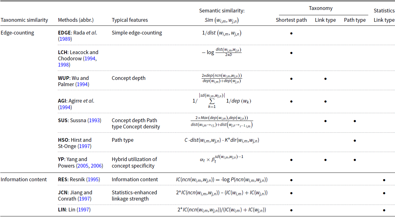
On the assumption of representing word meanings in the handcrafted semantic networks, taxonomic similarity measures, as listed in Table 1, can work effectively in predicting semantic similarity and can be generalized with three factors: the shortest path length, the link type and the path type, among which the shortest path length makes a major contribution to yield semantic similarity. To calculate the shortest path length, EDGE and LCH only hypothesize the uniform distance with the simple edge-counting, whereas WUP, YP and IC: RES, JCN and LIN also leverage taxonomy structures and word usage frequencies to fine-tune the uniform distance. Besides, HSO and YP factor in the path type in mixing the IS-A and HAS-A hierarchies to enrich semantic connections. Aside from the shortest path length in semantic networks, the key difference among taxonomic similarity methods is how to estimate concept specificity, either using network structures in edge-counting or using concept frequencies in IC.

Table 1. Summarization of the taxonomic similarity measures.

4.1. Distributional semantics

NNEs or the prediction-based embeddings – as a cornerstone of state-of-the-art distributional semantics – have significantly improved downstream NLP tasks (Collobert et al. Reference Collobert, Weston, Bottou, Karlen, Kavukcuoglu and Kuksa2011; Baroni et al. Reference Baroni, Dinu and Kruszewski2014). In contrast to the traditional counting-based distributional semantics such as pointwise mutual information (PMI) and latent semantic analysis (LSA) (Deerwester et al. Reference Deerwester, Dumais, Landauer, Furnas and Harshman1990; Turney Reference Turney2001; Turney and Pantel Reference Turney and Pantel2010), NNEs can yield much denser word vectors with the reduce dimensionalities in an unsupervised way of learning. Note that the dimensionalities of NNEs can impose a varied impact on their quality, which are often customized for different needs. However, the optimal NNEs, training results of dimensionality selection on one similarity task, often generalized poorly when testing on other similarity tasks or applications (Yin and Shen Reference Yin and Shen2018; Raunak et al. Reference Raunak, Gupta and Metze2019). As for prediction-based embeddings, we aim to examine the publicly available NNEs that have been well trained and widely adopted for transfer learning in NLP. Since optimizing dimensionality for NNEs is not a primary goal in this research, we keep their original sizes of dimensions untouched. We mainly embraced three types of NNEs in the evaluation.

4.2. Unified NNEs

We selected two NNEs: Skip-gram with Negative Sampling (SGNSFootnote ¹ ) (Mikolov et al. Reference Mikolov, Chen, Corrado and Dean2013a, Mikolov et al. Reference Mikolov, Sutskever, Chen, Corrado and Dean2013b) and GloVeFootnote ² (Pennington et al. Reference Pennington, Socher and Manning2014) for comparison, along with another well-known SGNS-based model – fastTextFootnote ³ (Bojanowski et al. Reference Bojanowski, Grave, Joulin and Mikolov2017). fastText aims to solve the widespread out-of-vocabulary (OOV) problem in NNEs through sub-word or n-gram character embeddings. In the word similarity and analogy tasks, Levy et al. (Reference Levy, Goldberg and Dagan2015) systematically contrasted SGNS and GloVe with two counting-based distributional semantics: PMI and truncated singular value decomposition (SVD). They concluded that fine-tuning hyperparameters during the NNEs’ training might contribute to their superiority over the counting-based models. Note that word embeddings derived from these NNEs are unified, which implies that different senses of a word share a uniform representation without sense disambiguation. We repeatedly tested the NNEs using different sizes of dimensionalities in the evaluation and only reported their optimal results for brevity.

4.3. Fusion of semantic relationships and NNEs

NNEs inclined to elicit semantic relatedness rather than semantic similarity (Hill et al. Reference Hill, Reichart and Korhonen2015; Lê and Fokkens Reference Lê and Fokkens2015) because they were trained unsupervisedly with word co-occurrences in a context window. They can hardly distinguish synonyms from antonyms, an easy task for taxonomic similarity models. Some studies further fed the advanced co-occurrence information such as syntactic dependency (Levy and Goldberg Reference Levy and Goldberg2014a) and sentiment information among linguistic units (Tang et al. Reference Tang, Wei, Yang, Zhou, Liu and Qin2014) into training NNEs. However, the results showed that such enrichment processes only played a limited role in improving NNEs on similarity prediction.

Another way of improving NNEs is to incorporate semantic relationships in LKBs by pulling synonyms deliberately closer in a latent semantic space. For example, using synonymous pairs extracted from WordNet and the Paraphrase databases (Ganitkevitch et al. Reference Ganitkevitch, VanDurme and Callison-Burch2013), Yu and Dredze (Reference Yu and Dredze2014) attempted to regularize the log-probability loss function during training NNEs; and Faruqui et al. (Reference Faruqui, Dodge, Jauhar, Dyer, Hovy and Smith2015) designed an efficient way of retrofitting word embeddings after training NNEs. PARAGRAM (Wieting et al. Reference Wieting, Bansal, Gimpel and Livescu2015) only employed the Paraphrase databases in training a Skip-gram initialized word embedding.

Apart from post-processing or retrofitting NNEs with synonyms, Mrkšić et al. (Reference Mrkšić, Ó Séaghdha, Thomson, Gasic, Rojas-Barahona, Su, Vandyke, Wen and Young2016) further took into account antonymous relationships – dubbed as counter-fitting (CF) – to push antonyms away during updating NNEs. They found that CF GloVe and PARAGRAM significantly improved their performances in predicting semantic similarity. Mrkšić et al. (Reference Mrkšić, Vulić, Ó Séaghdha, Leviant, Reichart, Gašić, Korhonen and Young2017) also employed multilingual semantic relationships in BabelNet (Navigli and Ponzetto Reference Navigli and Ponzetto2012a) during CF NNEs and gained an improvement on the cross-lingual semantic similarity tasks. The procedure of CF (Mrkšić et al. Reference Mrkšić, Ó Séaghdha, Thomson, Gasic, Rojas-Barahona, Su, Vandyke, Wen and Young2016) is to first extract external semantic constraints: synonyms S and antonyms A from LKBs, which are then used to update the original vector space R through a contrastive loss L. To derive the retrofitted space R ^* , CF defines L as follows:

\begin{align*}L = {L_S}\left( {{B_S}} \right) + {L_A}\left( {{B_A}} \right) + {L_P}\left( {R,{R^{\rm{*}}}} \right), \textrm{where}\end{align*}

• • B _S and B _A are two sets storing the external constraints S and A, respectively. For each synonymous or antonymous word pair (l, r) in the sets, CF updates its corresponding vectors ( $X^{\prime}_l$ , $X^{\prime}_r$ ) in R ^* with backpropagation;

• • ${L_S}\left( {{B_S}} \right) = \mathop \sum \nolimits_{\left( {l,\;r} \right) \in {B_S}} \tau \left( {{\delta _{syn}} - cos\left( {X_l^{\prime},X_r^{\prime}} \right)} \right)$ , calculating the loss L _S to make synonymous vectors alike in R ^* . $\tau \left( x \right) = max\left( {0,x} \right)$ is the hinge loss function. $\delta_{syn}$ denotes the maximum margin of similarity score that $X^{\prime}_l$ and $X^{\prime}_r$ can have. A part of the training objective of CF is to maximize distributional similarity between $X^{\prime}_l$ and $X^{\prime}_r$ to approach $\delta_{syn}$ or to pull $X^{\prime}_l$ and $X^{\prime}_r$ in R ^* close enough to one direction. $\delta_{syn}$ is adjustable for different tasks;

• • ${L_A}\left( {{B_A}} \right) = \mathop \sum \nolimits_{\left( {l,\;r} \right) \in {B_A}} \tau \left( {{\delta _{ant}} + cos\left( {X_l^{\prime},X_r^{\prime}} \right)} \right)$ , calculating the loss L _A to make antonymous vectors reciprocal in R ^*. In contrast to $\delta_{syn}$ , $\delta_{ant}$ is the minimum margin of similarity score that $X^{\prime}_l$ and $X^{\prime}_r$ can have. $\delta_{ant} = 0$ indicates that CF intends to train distributional similarity between $X^{\prime}_l$ and $X^{\prime}_r$ close to 0 or to push l and r in R ^* to a vertical direction;

• • ${L_P}\left( {R,{R^*}} \right) = \mathop \sum \nolimits_{i = 1}^{\left| V \right|} \mathop \sum \nolimits_{j \in Neg\left( i \right)} \tau \left( {cos\left( {{X_i},{X_j}} \right) - cos\left( {X_i^{\prime},X_j^{\prime}} \right)} \right)$ , preserving distributional distance learned in R when updating R ^* with semantic constraints of B _S and B _A . V is the vocabulary in R. For a word i in V, CF first retrieves a group of its negative sample words (Neg(i)) that are within a threshold of distributional similarity between i and j and then keeps their respective semantic distance in R and R ^* as same as possible.

• • L _S , L _A and L _P can have different weights in retrofitting NNEs for a specific task, and other semantic relationships such as IS-A and PART-OF can also be incorporated in L.

More recent studies showed moderate success in using multiple LKBs to retrofit NNEs. For example, Speer and Chin (Reference Speer and Chin2016) utilized an ensemble method of merging GloVe and SGNS with the Paraphrase databases and ConceptNet (Speer and Havasi Reference Speer and Havasi2012); Ponti et al. (Reference Ponti, Vulić, Glavaš, Mrkšić and Korhonen2018) employed generative adversarial networks to combine WordNet and Roget’s thesaurus with NNEs; Shi et al. (Reference Shi, Chen, Zhou and Chang2019) demonstrated some positive effects of retrofitting paraphrase contexts into NNEs.

Given its significant gains in semantic similarity prediction, we chose PARAGRAM+CFFootnote ⁴ (Mrkšić et al. Reference Mrkšić, Ó Séaghdha, Thomson, Gasic, Rojas-Barahona, Su, Vandyke, Wen and Young2016) – imposing semantic constraints on PARAGRAM with antonyms in WordNet and the Paraphrase databases – to investigate the fusion effect of integrating semantic relationships into NNEs.

4.4. Contextualized NNEs

In the unified (Bengio et al. Reference Bengio, Ducharme, Vincent and Janvin2003; Collobert et al. Reference Collobert, Weston, Bottou, Karlen, Kavukcuoglu and Kuksa2011; Mikolov et al. Reference Mikolov, Sutskever, Chen, Corrado and Dean2013b; Pennington et al. Reference Pennington, Socher and Manning2014) and hybrid (Faruqui et al. Reference Faruqui, Dodge, Jauhar, Dyer, Hovy and Smith2015; Wieting et al. Reference Wieting, Bansal, Gimpel and Livescu2015; Mrkšić et al. Reference Mrkšić, Ó Séaghdha, Thomson, Gasic, Rojas-Barahona, Su, Vandyke, Wen and Young2016) NNEs, a polysemous word shares a uniform embedding without any sense distinction. An ongoing research trend on NNEs has attended to cultivating contextualized embeddings using NLMs, for example, CoVe (McCann et al. Reference McCann, Bradbury, Xiong and Socher2017), ELMo (Peters et al. Reference Peters, Neumann, Iyyer, Gardner, Clark, Lee and Zettlemoyer2018a), ULMFiT (Howard and Ruder Reference Howard and Ruder2018), GPT-2 (Radford et al. Reference Radford, Wu, Child, Luan, Amodei and Sutskever2018) and BERT (Devlin et al. Reference Devlin, Chang, Lee and Toutanova2018). The contextualized embeddings leverage word order in contexts – often neglected in the static or unified NNEs – through deeper neural networks such as bidirectional RNN and Transformer with attention mechanism (Vaswani et al. Reference Vaswani, Shazeer, Parmar, Uszkoreit, Jones, Gomez, Kaiser and Polosukhin2017). They have greatly improved many natural language understanding tasks. For example, BERT – using both masked language modelling and sentence prediction in pre-training – had attained cutting-edge performance on some benchmark tasks such as GLUE (Wang et al. Reference Wang, Singh, Michael, Hill, Levy and Bowman2018) and SQuAD (Rajpurkar et al. Reference Rajpurkar, Zhang, Lopyrev and Liang2016).

The impressive results of these contextualized NNEs (hereafter CNNEs in short) can be attributed to the utilization of deep and multi-layered neural architectures such as CNNs, RNNs and Transformers. Such architectures can not only produce context-dependent word embeddings but also display various linguistic features in their respective layers (Peters et al. Reference Peters, Neumann, Zettlemoyer and Yih2018b; Goldberg Reference Goldberg2019; Tenney et al. Reference Tenney, Xia, Chen, Wang, Poliak, McCoy, Kim, Van Durme, Bowman, Das and Pavlick2019). Analogously, deep learning architectures on computer vision and ImageNet (Russakovsky et al. Reference Russakovsky, Deng, Su, Krause, Satheesh, Ma, Huang, Karpathy, Khosla, Bernstein, Berg and Fei-Fei2014) can learn multi-grained hierarchical features, from specific edges to general and abstractive patterns in images (Krizhevsky et al. Reference Krizhevsky, Sutskever and Hinton2012; Yosinski et al. Reference Yosinski, Clune, Bengio and Lipson2014). For the linguistic features learned from BERT, Jawahar et al. (Reference Jawahar, Sagot and Seddah2019) demonstrated in a series of probing tasks that its lower layers could contain morphological information and the middle layers and upper layers could capture syntactic and semantic information, respectively. Ethayarajh (Reference Ethayarajh2019) also showed that the upper layers in ELMo, BERT and GPT-2 might contain more task or context-specific information than the lower ones.

Among these deep learning CNNEs, we chose BERT-baseFootnote ⁵ rather than BERT-large in the evaluation. Even when BERT-base was pre-trained with a much less complicated structure than BERT-large (a sophisticated variant of BERT), it maintained competitive performance on some benchmark tasks. Throughout the evaluation, we used BERT to refer to BERT-base.

Unlike the unified word representations in NNEs, we used BERT to generate the sense representations of a polysemous word although such generation can only signify context-dependent word meanings at most. Directly feeding a word without its contexts into BERT would only retrieve implausible sense representations, equivalent to the unified NNEs in essence. We might employ a synset’s example sentences in WordNet as a proxy to its contexts, but nearly 50% of the nouns and 7% of the verbs in the evaluation datasets are lack of example sentences. We, therefore, replaced them with a synset’s gloss as the input of BERT. For each synset of a word, we averaged the vectors of all the tokens in its corresponding gloss to yield an aggregated embedding, which can function as the sense embedding of a word. We then defined semantic similarity between a pair of words as the maximum of distributional similarity scores (cosine) across their sense embeddings in BERT, derived in the same way as the maximum of taxonomic similarity across different senses in Section 3. Given that the top layers in BERT are more context-specific and semantics-oriented, we first individually calculated the sense embeddings of a synset from the 9^th to 12^th layer, together with an average embedding on the four layers. Among these five embeddings, we only highlighted the best, achieved on the 11^th layer, in the evaluation.

5.1. Human similarity judgements

Human similarity judgements are often acquired in a context-free setting where it is common for the lack of corresponding contextual hints to help disambiguate word meanings. With both context and non-context aiding, Resnik and Diab (Reference Resnik and Diab2000) designed a pilot dataset only consisting of forty-eight verb pairs. In their pioneering work, they found that taxonomic similarity models (i.e., EDGE, RES and LIN) worked likewise in the non-context setting, whereas they all improved to some degree in the context setting. Their results indicated that human subjects might comprehend word meanings more arbitrarily when corresponding contextual hints were absent. Given the complexity and laboriousness of constructing datasets in the context setting, nearly all the current datasets in use, for example, SimLex-999 (Hill et al. Reference Hill, Reichart and Korhonen2015) and SimVerb-3500 (Gerz et al. Reference Gerz, Vuli’c, Hill, Reichart and Korhonen2016), are context-free. They were dedicatedly designed for measuring semantic similarity rather than semantic association (Hill et al. Reference Hill, Reichart and Korhonen2015). Note that hereafter to name a dataset, the initial numbers stand for its size, followed by its PoS tag. We only collected some context-free datasets for evaluation. They consisted of two datasets on nouns (N): 65_N (Rubenstein and Goodenough Reference Rubenstein and Goodenough1965) and the similarity subset of 201_N (Agirre et al. Reference Agirre, Alfonseca, Hall, Strakova, Pasca and Soroa2009) – extracted from 353_N (Finkelstein et al. Reference Finkelstein, Gabrilovich, Matias, Rivlin, Solan, Wolfman and Ruppin2001); two on verbs (V): 130_V (Yang and Powers Reference Yang and Powers2006) and 3000_V – the test part of SimVerb-3500; only one containing both nouns, verbs and adjectives (ALL) – 999_ALL, that is, SimLex-999. We further extracted two subsets from 999_ALL: 666_N and 222_V.

5.2. Definition of an upper bound

Past studies defined an upper bound in evaluation via average correlation coefficients (Spearman’s $\rho$ or Pearson’s r) among pairwise annotators or between a leave-one-out annotator and group average. Such a definition on the upper bound is often problematic because it can be surpassed or reached with a proximity to humans. For example, using their hybrid taxonomic similarity model, Yang and Powers (Reference Yang and Powers2005) achieved r = 0.92 on 30_N (Miller and Charles Reference Miller and Charles1991), surpassing the upper bound of r = 0.90 in the pairwise agreement. Recski et al. (Reference Recski, Iklódi, Pajkossy and Kornai2016) designed a regression model combining multiple distributional similarity models, taxonomy features and features extracted from a concept dictionary. They achieved $\rho = 0.76$ on 999_ALL, well exceeding the upper bound of $\rho = 0.67$ in the pairwise agreement and close to the group average of $\rho = 0.78$ . These excellent results need to be interpreted with due care because it does not mean their methods (Yang and Powers Reference Yang and Powers2005; Recski et al. Reference Recski, Iklódi, Pajkossy and Kornai2016) have gone beyond human similarity judgements. It only suggests that they could achieve more accurate results than most of the individual annotators on the specific datasets. As noticed by Lipton and Steinhardt (Reference Lipton and Steinhardt2018), before we can understand the internal mechanism of human similarity judgements, we should employ extreme caution in using ‘human-level’ terms in describing computational models or claiming their supremacy over humans. Therefore, an upper bound needs to be established properly.

We suggest that the upper bound should be taken as an average agreement among different human groups on the same task (groupwise agreement), through which we can correctly set up a maximum on similarity judgements. For example, Rubenstein and Goodenough (Reference Rubenstein and Goodenough1965) hired 51 college undergraduates to evaluate their well-known 65_N; and Miller and Charles (Reference Miller and Charles1991) extracted 30 pairs from 65_N and repeated a similar experiment with 38 subjects. As for 65_N and 30_N, where human similarity scores are evenly distributed from high to low, the correlation coefficient between the mean human ratings of the two groups is r = 0.97 or $\rho = 0.95$ . Moreover, Resnik (Reference Resnik1995) replicated an experiment on the 28 pairs extracted from 30_N. He hired 10 subjects and achieved r = 0.96 or $\rho = 0.93$ between the mean human ratings of 28_N and 30_N. Therefore, the upper bound for judging noun similarity should approximate r = [0.96, 0.97] or $\rho = [0.93, 0.95]$ . Analogously, to estimate the upper bound on the verb task, we calculated a groupwise agreement on the 170 verb pairs that occurred in both 999_ALL (50 participants) and SimVerb-3500 (843 participants), which stands at r = 0.92 or $\rho = 0.91$ (Gerz et al. Reference Gerz, Vuli’c, Hill, Reichart and Korhonen2016). Given the reasonably large number of participants in the experiments, these values can serve as the reliable upper bounds in the evaluation.

5.3. Results on intrinsic evaluation

Note that in the following sections, we solely reported Spearman’s rank correlation on head-to-head comparisons as it makes no assumptions of linear dependence on similarity scores.

As indicated in the heat map of Figure 2, the group performance (mean 0.56, 95% confidence interval (CI) 0.47 to 0.65) of the taxonomic similarity measures was on average better than that (mean 0.47, 95% CI 0.34 to 0.62) of SGNS, fastText, GloVe and BERT. This finding is in line with the previous studies on NNEs (Hill et al. Reference Hill, Reichart and Korhonen2015; Lê and Fokkens Reference Lê and Fokkens2015). Except for PARAGRAM+CF, the two groups of similarity measures could be roughly divided into two corresponding clusters in the dendrogram of Figure 2, apparently showing distinctive patterns over the seven datasets. PARAGRAM+CF with a mean correlation of 0.71 (95% CI 0.68 to 0.75) was substantially different from both groups in Figure 2.

Figure 2. Comparison of the taxonomic and distributional similarity measures on the seven benchmark datasets (in terms of Spearman’s $\rho$ ). We attached the heat map (top left) with a dendrogram of the measures. We applied a hierarchical clustering using average linkage and Pearson distance on the measures. The boxplot (bottom left) shows the variation of each measure’s correlations across the seven datasets. The column chart (bottom right) further indicates the performance variation of each measure on the group-aggregated level of nouns (65_N, 201_N and 666_N) and verbs (130_V, 222_V and 3000_V).

Moreover, edge-counting and IC showed no significant pattern differences in Figure 2 (Friedman test: χ² = 7.65, p = 0.37). The result partly supports our hypothesis on the prime role of the shortest path length in calculating taxonomic similarity and suggests that only a minor role of the link or path type can play in adjusting the uniform distance. Except for PARAGRAM+CF, no significant differences existed among NNEs (Friedman test: χ² = 3.51, p = 0.32).

PARAGRAM+CF tends to have a more consistent similarity prediction with a standard deviation of 0.06 (95% CI 0.02 to 0.08) than other measures across the seven datasets and performed competently well above others on 65_N, 666_N, 222_V and 3000_V. It also outperformed others on 999_ALL, the only dataset containing both nouns, verbs and adjectives. In general, PARAGRAM+CF, retrofitting multiple semantic relationships in LKBs into NNEs, improved the capability of distributional vector models in yielding semantic similarity, which corroborates previous findings in the literature (Faruqui et al. Reference Faruqui, Dodge, Jauhar, Dyer, Hovy and Smith2015; Mrkšić et al. Reference Mrkšić, Ó Séaghdha, Thomson, Gasic, Rojas-Barahona, Su, Vandyke, Wen and Young2016; Mrkšić et al. Reference Mrkšić, Vulić, Ó Séaghdha, Leviant, Reichart, Gašić, Korhonen and Young2017).

Concerning a method’s divergence on the group average performance, we first defined its mean correlation ratio (MCR in short) from noun to verb task to quantify performance variability. As shown in the column chart in Figure 2, the MCR of PARAGRAM+CF (1.10) was only larger than that of JCN (1.00) and LIN (1.01), which possibly indicates a similar level of variability in similarity prediction. EDGE, WUP, LCH, RES, HSO and YP ([1.24, 1.48]) had relatively lower MCRs than SGNS, GloVe, fastText and BERT ([1.47, 1.96]), which implies that taxonomic similarity could be on average more stable than NNEs. Overall, the MCRs also indicate that nearly all similarity measures (except for JCN and LIN) deteriorated by a certain degree from noun to verb task. The overall performance of these methods on the noun datasets (mean 0.63, 95% CI 0.60 to 0.66; standard deviation 0.06, 95% CI 0.03 to 0.08) was better than it on the verb ones (mean 0.48, 95% CI 0.43 to 0.53; standard deviation 0.10, 95% CI 0.06 to 0.13). The result suggests that it may be more challenging to compute verb similarity than noun similarity, to which a hybrid use of neural embeddings and semantic relations, for example, PARAGRAM+CF, may provide a solution.

5.4. Noun and verb similarity

Apart from a performance overview of these measures on the seven benchmark datasets, we further pinpoint their detailed differences on yielding semantic similarity on nouns and verbs in the datasets: 666_N and 3000_V, respectively. We propose three criteria, word frequency, polysemy degree and similarity intensity, to investigate their effects on similarity prediction.

5.4.1. Word frequency

Word frequency is highly associated with synset ranking in WordNet. Frequency statistics also have a crucial application in similarity calculation, such as factoring in concept specificity with IC and pre-training neural embeddings. To investigate word frequency’s effect on similarity judgements, we first set up three intervals that cover word usages from low-, medium- to high-frequency ranges, sampled from BNC. We then extracted word pairs from each dataset with their word occurrence numbers that are both sat in one of the three intervals.

As shown in Table 2, EDGE and LCH – only employing the shortest path length in WordNet – were little sensitive to the frequency variations on both datasets (SE ≤ 0.01), and each of them was not significantly different for the frequency ranges on 666_N (one-way ANOVA: EDGE: F(2, 232) = 1.06, P = 0.35; LCH: F(2, 232) = 1.74, P = 0.18) and 3000_V (one-way ANOVA: EDGE: F(2, 1072) = 0.15, P = 0.86; LCH: F(2, 1072) = 0.32, P = 0.72). Although the link type and path type have impacts on adjusting the uniform distance, IC: RES, JCN and LIN, together with edge-counting: WUP, HSO and YP, showed no significant performance variations over the frequency intervals, as determined by one-way ANOVA (P > 0.05). Except for PARAGRAM+CF, YP also attained the best in each of the intervals with a consistent performance on 666_N (SE = 0.00), but it showed a little fluctuation on 3000_V (SE = 0.03) despite no significance (one-way ANOVA: F(2, 1072) = 0.34, P = 0.72).

Table 2. Word frequency’s effects on yielding semantic similarity. For the noun pairs in 666_N (left), we first divided their frequency range into three intervals: less than 3,000; between 3,000 and 10,000; and more than 10,000. We then individually acquired 61, 104 and 70 noun pairs that can satisfy the frequency requirements of the three intervals. Likewise, in 3000_V (right), 449, 355 and 275 pairs of verbs were respectively extracted for the three frequency intervals: less than 1,000; between 1,000 and 5,000; and more than 5,000. We also added the overall results on 666_N and 3000_V for reference.

NNEs including SGNS, GloVe and fastText, along with PARAGRAM+CF, were more sensitive to the frequency variations on 666_N (SE: [0.03, 0.06]) than on 3000_V (SE: [0.01, 0.02]), but such sensitivity was not significant, according to one-way ANOVA (P > 0.05). However, fastText (one-way ANOVA: F(2, 1072) = 8.27, P = 0.00), PARAGRAM+CF (one-way ANOVA: F(2, 1072) = 5.60, P = 0.00) and GloVe (one-way ANOVA: F(2, 1072) = 4.61, P = 0.01) showed significant performance variations on 3000_V, except for SGNS (one-way ANOVA: F(2, 1072) = 1.90, P = 0.15). Overall, PARAGRAM+CF achieved better results than YP, the best in edge-counting, excluding the low frequency range on 666_N. In contrast to other NNEs, BERT was less subject to the frequency change (SE = 0.01, one-way ANOVA: F(2, 232) = 2.09, P = 0.13 on 600_N and SE = 0.01, F(2, 1072) = 0.38, P = 0.69 on 3000_V).

Note that apart from the five datasets in our evaluation, mainly consisting of frequent words in generic domains, there are other benchmark similarity datasets such as RW-2034 (Luong et al. Reference Luong, Socher and Manning2013) and CARD-660 (Pilehvar et al. Reference Pilehvar, Kartsaklis, Prokhorov and Collier2018). They were particularly designed to cover infrequent or rare words, which were retrieved from extremely larger sizes of corpora than BNC. They are often taken to validate NNEs’ quality, especially in dealing with OOV words. Although fastText and BERT can address the OOV issue through sub-word encoding, the other NNEs in the evaluation, along with taxonomic measures, are still subject to the limited sizes of their vocabularies. We therefore extracted two subsets of 349 and 52 word pairs from RW-2034 and CARD-660, respectively, in which all the measures can yield corresponding similarity scores on any target pair.

As shown in Figure 3, taxonomic similarity achieved better results on CARD-660 (mean±SD: 0.46±0.11) than on RW-2034 (0.27±0.05), whereas NNEs performed adversely with 0.01±0.07 on CARD-660 and 0.45±0.16 on RW-2034. PARAGRAM+CF (0.58), along with SGNS (0.58), surpassed the other measures on RW-2034, but it plummeted to 0.15 on CARD-660, sharply lower than taxonomic measures and modestly higher than the other NNEs. In line with the results on the low frequency ranges on 666_N and 3000_V in Table 2, taxonomic similarity measures were relatively stable on calculating similarity on rare words, but NNEs fluctuated sharply. Given that our findings are based on a limited number of rare words, and the upper bounds (around 0.43 and 0.90, respectively) on RW-2034 and CARD-660 are substantially different, the results on a small scale of coverage should therefore be treated with considerable caution. For reasons of space, a further investigation into rare words is reserved for future work.

Figure 3. Yielding semantic similarity on rare words.

Our findings suggest that taxonomic similarity may be neutral to the variations of word frequency, partly because edge-counting mainly relies on semantic networks to calculate the shortest path length; partly because IC may ineffectively estimate concept specificity in adjusting the uniform distance. As the neural embeddings are the results of pre-training neural networks with co-occurrences, their performances may be susceptible to the frequency variations. Especially for words with higher frequencies, their corresponding neural embeddings may put them into a better position in yielding semantic similarity.

5.4.2. Polysemy degree

In WordNetFootnote ⁶ , nouns have 2.79 senses on average and verbs 3.57. With the increase of a word’s polysemy degree, sense disambiguation would become more demanding, and searching the shortest path would engage in more path options in a taxonomy. It may result in a potential misestimation of taxonomic similarity and incorrect identification of authentic word senses in contexts. Additionally, the more senses a word owns implies the more idiosyncratic context patterns it will have. Assembling these patterns in a uniform representation may undermine the representability of distributional vector models in deriving semantic similarity.

As shown in Table 3, all the taxonomic similarity measures worsened off while working on the highly polysemous nouns. However, one-way ANOVA indicates that their performance variations (SE = 0.03 on average) on the polysemy degree were not significant (P > 0.05). By contrast, they were less varied on the polysemous verbs (SE = 0.01 on average) but with a significant difference ( $P \ll 0.05$ , one-way ANOVA). The result implies that the highly polysemous nouns tend to have more complex interconnections in semantic networks, which can be problematic to search the shortest path effectively and then yield similarity scores correctly; the shallow and simple verb hierarchy may lessen the impact of polysemy degree on similarity calculation.

Table 3. Polysemy degree effects on judging semantic similarity. On 666_N (left), we divided polysemy degree into three intervals: less than or equal to 2 in sense numbers, between 2 and 4, and more than 4, in which we finally retrieved 91, 152 and 102 noun pairs, respectively. On 3000_V (right), we retrieved 344, 480 and 319 verb pairs according to the sense number intervals: less than 3, between 3 and 8, and more than 8, respectively. We also added the overall results on 666_N and 3000_V for reference.

Interestingly, the polysemy degree tallied with the performance of each NNE on 3000_V, that is, the less sense number or weaker polysemy degree indicates the more accurate outcomes on similarity prediction (P << 0.05, one-way ANOVA). This finding is in line with the previous work on the polysemy effects on distributional similarity (Gerz et al. Reference Gerz, Vuli’c, Hill, Reichart and Korhonen2016). Among NNEs, PARAGRAM+CF performed the best on each level of polysemy degree. The sense or contextualized embeddings, generated by BERT, outperformed the unified NNEs: SGNS, GloVe and fastText on the medium and high ranges of polysemy degree on 3000_V, but not on the high range on 666_N.

Overall, in Table 3, when words become less polysemous or conceptually coarse-grained, both taxonomic similarity and neural embeddings can perform better on similarity prediction. Retrofitting NNEs with handcrafted semantic networks can enhance distributional vector models in predicting semantic similarity on different levels of polysemy degree.

5.4.3. Similarity intensity

The 10-point Likert scale similarity scores in the gold standard datasets, ranging from the highest (10) for synonyms or near-synonyms to the lowest for antonyms (0), can signify not only words’ interchangeability in contexts but also their semantic nuances. In leveraging handcrafted semantic relationships, taxonomic similarity can set up different weighting factors such as the link and path type to approach similarity intensity appropriately. By contrast, under the premise of similar words sharing similar contexts (Firth Reference Firth1957), distributional similarity only depends on co-occurrence patterns in estimating similarity intensity. As synonyms and antonyms often share similar contextual patterns, distributional similarity may not differentiate them effectively without the aid of additional resources and attempts to score them both highly related.

As for 666_N in Table 4, all the measures worked significantly better in the low range of similarity intensity (mean±SE: 0.53±0.01) than in the medium (0.15±0.02) and high (0.29±0.02) ranges ( $P \ll 0.05$ , one-way ANOVA). Moreover, in the medium range, all the taxonomic similarity measures achieved higher correlation values than the neural embeddings, except for PARAGRAM+CF. Results on 3000_V in Table 4 also show that PARAGRAM+CF outperformed all other measures across the three ranges; on the high range, except for PARAGRAM+CF, all the measures achieved a significant net gain (P << 0.05, one-way ANOVA). Overall, all the measures, except for HSO, performed worst in the medium range on 666_N and 3000_V.

Table 4. Similarity intensity effects on judging semantic similarity. On 666_N (left), we divided the gold standard similarity scores into three intensity ranges: less than 3, between 3 and 6, and more than 6, and each range contains 200, 267 and 199 pairs, respectively. On 3000_V (right), 1,089, 1,033 and 878 pairs were individually extracted from the three ranges. As for each method, the dark red error bar indicates its mean and standard error. We also added the overall results on 666_N and 3000_V for reference.

Our findings indicate that the taxonomic similarity measures failed to perform consistently on different levels of similarity intensity, which may be partly caused by the synset organization in WordNet. For example, on the high range of similarity intensity, only 15.6%, 26.6% and 25.6% of word pairs (a total of 67.8%) in 666_N have the shortest path length of zero (synonyms), one and two links in edge-counting, respectively; and so do 27.9%, 30.4% and 18.5% of word pairs (a total of 76.9%) in 3000_V. The domain and coverage of existing LKBs, purpose-built by lexicographers, only recorded a relatively stable vocabulary knowledge (Kilgarriff Reference Kilgarriff1997; Kilgarriff and Yallop Reference Kilgarriff and Yallop2000), which are diversified on the compilation of synonyms or near-synonyms. WordNet only organized paradigmatic relations into a fine-grained semantic network where the words in a synset node strictly conform to the notion of semantic similarity or interchangeability in contexts (Kilgarriff and Yallop Reference Kilgarriff and Yallop2000). Conversely, as for Roget’s tree structure in both paradigmatic and syntagmatic relations, each node contains highly related words. The unbalanced distribution of highly similar words in WordNet may impose a constraint on the effect of edge-counting, dampening the conditioning effects of the link and path type on the uniform distance. The hybrid use of concept relationships and distributional semantics, for example, PARAGRAM+CF, may address the unbalanced and outdated structure issue of LKBs in deriving semantic similarity.

5.4.4. Results aggregation

After investigating these measures under the conditions of word frequency, polysemy degree and similarity intensity on 666_N and 3000_V, we assembled their results to further compare their patterns in similarity prediction. Figure 4 displays that the group: EDGE, WUP, LCH, JCN and LIN, forming a hierarchical cluster, shared a similar pattern of performances on 666_N and 3000_V (Friedman test: χ² = 7.50, p = 0.11), so did the group of RES and HSO (Friedman test: χ² = 1.03, p = 0.60). As for IC, no significant pattern differences existed between JCN and LIN (Friedman test: χ² = 1.00, p = 0.45). The neural embedding group, including SGNS, GloVe, fastText and BERT, also demonstrated a significantly similar pattern (Friedman test: χ² = 0.91, p = 0.63), but PARAGRAM+CF distanced itself from any group, which is in good agreements with our findings in Figure 2.

Figure 4. An overview of the effects of word frequency (WF), polysemy degree (PD) and similarity intensity (SI) on similarity judgements. For each column name, N and V denote the two datasets: 666_N and 3000_V, respectively. We added a dendrogram of the similarity measures, using average linkage and Euclidean distance.

The aggregated results in Figure 4 are consistent with the previous findings, which in general suggest that the taxonomic similarity measures can outperform the unified and contextualized neural embeddings in similarity prediction. Additionally, the simple edge-counting can effectively yield semantic similarity without using the conditioning factors on the uniform distance. PARAGRAM+CF, retrofitting NNEs with multiple semantic relations such as synonyms and antonyms, can pave a new way of combining taxonomic and distributional similarity to improve semantic similarity prediction.

6.1. Taxonomic similarity

As shown in Figure 5, all the taxonomic similarity measures worked likewise on 666_N (mean 0.80, 95% CI 0.76 to 0.83) and 3000_V (mean 0.79, 95% CI 0.76 to 0.82), among which EDGE, WUP and LCH were extraordinarily close with a mean $\rho$ of 0.98 (SE = 0.01) and 0.91(SE = 0.03) on 666_N and 3000_V, respectively, and so were LIN and JCN with $\rho = 0.97$ and $\rho = 0.94$ . Additionally, in comparison with human judgements, these measures, as a single group, also showed a similar pattern over the subsets of 666_N and 3000_V in Figure 5. Overall, the results on mutual proximity suggest that both the edge-counting and IC models may behave less distinctively in predicting semantic similarity, although multiple factors such as concept depth and frequency can be applied to differentiate the uniform distance. The simple edge-counting may prevail in calculating taxonomic similarity.

Figure 5. An overview of model proximity: 666_N (left) and 3000_V (right).

Our experiments are in line with previous findings on the effectiveness of concept specificity on taxonomic similarity measures (Jiang and Conrath Reference Jiang and Conrath1997; Lastra-Díaz and Garcia-Serrano Reference Lastra-Díaz and Garcia-Serrano2015), which may be strongly dependent on the organization of concept networks in mitigating the bias of uniform distance. Wang and Hirst (Reference Wang and Hirst2011) showed that concept density alone held no correlations with human similarity judgements, in which the uneven concept distribution in WordNet could result in a lack of information inheritance, also claimed by Resnik (Reference Resnik1995) in proposing IC. Concept density was then redefined through recursively adding information inheritance from a concept’s ancestors (hypernyms in the IS-A hierarchy) and concept depth through designing a cumulative distribution function. They attained a moderate improvement on the similarity measures of Wu and Palmer (Reference Wu and Palmer1994) and Jiang and Conrath (Reference Jiang and Conrath1997). Note that apart from the aforementioned concept depth and density in Section 3, other structural features in a taxonomy such as concept descendants (Seco et al. Reference Seco, Veale and Hayes2004), concept ancestors and even leaf nodes (Sánchez et al. Reference Sánchez, Batet and Isern2011) were also used to estimate concept specificity. Lastra-Díaz and Garcia-Serrano (Reference Lastra-Díaz and Garcia-Serrano2015) observed that merely minor differences existed while applying different strategies of intrinsic and extrinsic IC on the popular taxonomic similarity models in WordNet (Pedersen et al. Reference Pedersen, Patwardhan and Michelizzi2004). These past studies have suggested that the taxonomy structures in LKBs may constrain different hypotheses of concept specificity from adjusting the uniform distance, and therefore the shortest path length may be the only effective factor in measuring taxonomic similarity.

Moreover, previous tests (McHale Reference McHale1998; Jarmasz and Szpakowicz Reference Jarmasz and Szpakowicz2003), carried out for the adaptability of edge-counting, concurred with our initial results in the evaluation. Using Resnik’s 28 noun pairs (Reference Resnik1995), McHale (Reference McHale1998) tested the adaptability of the taxonomy similarity methods: EDGE, RES and JCN (without the intervention of concept depth and local concept density) in WordNet and Roget. He found that EDGE significantly outperformed RES and JCN in Roget with r = 0.89, although it was the worst with r = 0.67 in WordNet. RES achieved r = 0.79 in WordNet and performed nearly the same in Roget. As for JCN, the best correlation value was r = 0.83 in WordNet, which dropped to r = 0.79 in Roget. McHale claimed that the improvement of EDGE in Roget was partly due to its shallow structure – generally no more than eight levels; partly due to abundant lexical relationships (syntagmatic and paradigmatic). In contrast, WordNet is primarily equipped with the paradigmatic relationships of IS-A, and the 16 levels of IS-A hierarchy are relatively complicated. The moderately consistent results for RES, along with the slight variation of JCN in WordNet and Roget, indicated that they might be insensitive to the shortest path length in edge-counting, but might strongly depend on word usage statistics in practice. Jarmasz and Szpakowicz (Reference Jarmasz and Szpakowicz2003) also investigated the adaptability of EDGE in WordNet and Roget, along with other methods implemented in the similarity package of Pedersen et al. (Reference Pedersen, Patwardhan and Michelizzi2004). Their evaluation results on the 30_N (Miller and Charles Reference Miller and Charles1991) and 65_N partly fitted with McHale: for 30_N, EDGE outperformed others with $\rho = 0.87$ in Roget and arrived at moderate correlation with $\rho = 0.76$ in WordNet; for 65_N, it performed nearly identically in Roget ( $\rho = 0.81$ ) and WordNet ( $\rho = 0.80$ ). The findings on the adaptability of the taxonomic similarity models in WordNet and Roget demonstrated that the shortest path length alone in the simple edge-counting can predict word similarity as effectively as the other complicated measures that consider fine-tuning the uniform distance with concept specificity. Irrespective of the idiosyncratic organization of LKBs, the shortest path length can be a prime factor in modelling taxonomic similarity.

6.2. Distributional similarity in neural embeddings

In Figure 5, the neural embeddings, as a single group, demonstrated little interrelations with the taxonomic similarity measures on 666_N (mean 0.45, 95% CI 0.43 to 0.47) and 3000_V (mean 0.33, 95% CI 0.29 to 0.38), in which SGNS, GloVe and fastText were highly approximate to each other on 666_N (mean±SE: 0.83±0.01) and 3000_V (0.73±0.01). Similar results for the NNEs can also be found in Figure 4, in comparing with human similarity judgements on 666_N and 3000_V. The results showed that although different corpora and training methodologies were adopted in deriving distributional representations, SGNS, GloVe and fastText may bear a close resemblance in computing distributional similarity, which confirms the previous hypothesis that they function equivalently as a process of matrix factorization (Levy and Goldberg Reference Levy and Goldberg2014b; Levy et al. Reference Levy, Goldberg and Dagan2015). For example, in utilizing word co-occurrence matrix to yield neural embeddings, it has been demonstrated that SGNS works merely with factorizing a PMI transferred matrix (Levy and Goldberg Reference Levy and Goldberg2014b), and GloVe’s training objective is just to learn a factorization of a logarithmic matrix approximately (Levy et al. Reference Levy, Goldberg and Dagan2015).