INTRODUCTION
This paper takes a new look at the hysteresis hypotheses and provides new insights to evaluate the European unemployment problem. More precisely, the aim of this paper is to provide an explanation of the following two empirical regularities that existing literature has shown:1
Bianchi and Zoega (1998) show the existence of two regimes in the unemployment rate. Henry, Karanassou, and Snower (2000) and Karanassou, Sala, and Snower (2003) provide evidence on the relation between unemployment and capital accumulation.
The fact that European labor markets have never recovered the full employment levels that characterized the 1960s and first 1970s remains as one of the main puzzles in economics. The Structuralist approach [see Phelps (1994)] explains this puzzle arguing that the persistent increase in unemployment is the result of a combination of persistent shocks that raised the Natural Rate of Unemployment (NRU).2
See, for example, Hoon and Phelps (1992) and Phelps and Zoega (1998) for an analysis of the shocks explaining the rise in the NRU.
Blanchard and Summers (1988) argued that it was necessary to go beyond the natural rate hypothesis and concluded that “theories of fragile equilibria [a concept to highlight the sensitive dependence of unemployment on current and past events] are necessary to come to grip with events in Europe.” Despite this claim, the work on multiple equilibria has not played a major role in the literature. Two main contributions in this area are Diamond (1982) and Mortensen (1989), but in the context of search and matching models, which fall well apart from the dynamic general equilibrium approach we propose in this paper. From the more traditional perspective of the demand-supply side analysis, Manning (1990 and 1992) argued in favor of models with multiple equilibria to explain the postwar behavior of unemployment. Nonetheless, the mainstream literature on unemployment in the 1990s has kept apart from the multiple equilibria perspective and, following the work by Layard, Nickell, and Jackman (1991), has focused mainly on the NRU/NAIRU (i.e., a unique unemployment equilibrium rate), leaving also the hysteresis hypothesis a secondary role. Some work is, of course, being done on the hysteresis hypotheses, but mainly with an empirical concern.3
Some examples are Cross (1988 and 1995), and some papers therein that relate the hysteresis hypothesis with the NRU; Jaeger and Parkinson (1994) and, recently, Piscitelli, Cross, Grinfeld, and Lamba (2000), Hughes Hallet and Piscitelli (2002) and León-Ledesma and McAdam (2004), on the empirical testing of the hysteresis hypotheses.
The analysis of Bianchi and Zoega (1998) shows the existence of two regimes in the unemployment rate. This finding can be explained as the result of either an endogenous NRU or hysteresis. Moreover, the analysis of Phelps and Zoega (1998) rejects the possibility of extremely low speeds of convergence and, thus, does not support this explanation of hysteresis. This analysis, however, does not reject an explanation based on multiple equilibria, which is able to explain the persistence of temporary shocks even with high speeds of convergence. It follows that both, the multiple equilibria and the endogenous NRU approaches are plausible candidates to explain Bianchi and Zoega's (1998) findings.
Given the empirical bias of this work, the main sets of candidates for explaining hysteresis are still the ones initially proposed in Blanchard and Summers (1986 and 1987), a first one pointing to insider-outsider arguments, a second one to capital accumulation (either in the form of physical or human capital) and a third one to fiscal policy. In contrast with the extensive literature on the insider-outsider argument [see, among many others, Lindbeck and Snower (2001)], the other two explanations have received little relative attention in the theoretical literature. On the one hand, Coimbra, Lloyd-Braga and Modesto (2000) and Ortigueira (2003) are among the few exceptions arguing that a low accumulation of capital may explain persistent high unemployment rates.5
Like us, Coimbra et al. (2000) argue in favor of multiple steady states, but with an Overlapping Generations Model with strong increasing returns to scale, which are at odds with the empirical evidence [see Basu and Fernald (1997)]. In turn, our approach also differs from Ortigueira (2003), whose analysis is based on a model of labor search with frictional unemployment and human capital accumulation.
In contrast to the mainstream theoretical literature, generally overlooking the close relation displayed by the data between capital accumulation and unemployment,6
Some empirical literature shows that there is a close relationship between these two variables. This is outlined by Rowthorn (1999) who suggests “that a major factor behind persistent unemployment may also be inadequate growth in capital stock.” Henry, Karanassou, and Snower (2000) point to the importance of the role of capital stock in influencing the U.K. unemployment trajectory, but it is in Karanassou, Sala, and Snower (2003) that a reappraisal of the causes of European unemployment is provided, and capital stock is shown to be an important determinant (if not the leading one) of the movements in the European unemployment rate.
We show that fiscal policy explains hysteresis in a simple endogenous growth model with a linear aggregate production function, where the consumption-savings decision is taken by a representative infinitely lived dynasty. Unemployment arises from labor market imperfections introduced by assuming that unions set the wage to maximize an objective function depending on labor and the level of wages net of taxes relative to a reference wage level. Following de la Croix and Collard (2000), and subsequent work, the latter is identified as a stock of habits. The assumption on the unions' behavior implies that the solution to the maximization problem is a wage equation that sets the wage net of taxes as a constant markup over the reference wage. This introduces wage inertia because the reference wage is constructed as a weighted average of past labor income. To close the model, we assume that total government disbursements (i.e., government spending and unemployment benefits) are financed by means of both direct taxes and nondistortionary taxes, aiming to maintain a balanced budget rule. To this end, we assume that either government spending or direct taxes are endogenous and adjust to keep the budget constraint balanced. When government spending is treated as endogenous, direct tax rates are constant and, hence, exhibit an acyclical behavior. In contrast, when direct tax rates are considered endogenous, we expect them to be countercyclical; that is, to be high in bad times and low in good times. This is simply a result from the fact that public disbursements, such as unemployment benefits, rise in bad times and shrink in good times.7
Schmitt-Grohé and Uribe (1997) denote by endogenous taxes those taxes that adjust in order to balance the government budget constraint. They show that endogenous taxes cause the local indeterminacy of the equilibrium path in a neoclassical growth model with a perfectly competitive labor market.
When direct tax rates are assumed to be exogenous and constant, the higher is economic growth the higher capital accumulation and the more the labor demand shifts up. Thus, employment is enhanced, provided the rise in labor demand does not fully translate into wage increases, which happens when wage inertia is sufficiently strong. In Section 4, we show that the equilibrium path with exogenous taxes is unique and conclude that fails to explain hysteresis.
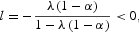
When direct tax rates are assumed to be endogenous, they generate a complementarity between capital accumulation and employment that makes agents' expectations self-fulfilling and, hence, generate multiple equilibrium paths. To see it, assume that agents coordinate into an expectations of high net interest rate. If agents are willing to substitute consumption intertemporally, the savings rate will be large and so will be the growth rates of capital stock and labor demand. When there is wage inertia, the latter implies high values of the employment rate and, thus, strong economic activity, implying large government revenues and low government expenditures. Obviously, the endogenous direct tax rate will be low in equilibrium and hence the equilibrium interest rate net of taxes will be large, which ensures that agents' expectations hold in equilibrium. This explains the existence of an equilibrium path corresponding to an economic regime of high economic activity and, analogously, the existence of another equilibrium path corresponding to a low regime. In Section 5, we show that the assumption of endogenous taxes may cause the existence of two different equilibrium paths converging to different steady states. One of them corresponds to a high regime characterized by high employment, savings and growth rates, and low direct tax rates; whereas the other one is a regime characterized by low employment, growth and savings rates, and high tax rates. Along these two equilibrium paths, government spending as a fraction of income is constant and, thus, both paths converge to different steady states that belong to different sides of the same Laffer curve. In this context, we interpret hysteresis as the result of equilibrium selection between these two paths.
The assumptions on the fiscal policy drive the transition. When tax rates are exogenous, employment and the savings rate are negatively related, as a larger employment rate causes a positive wealth effect that reduces the savings rate. In contrast, when tax rates are endogenous, employment and the savings rate display, along the two equilibrium paths, a positive correlation because of a substitution effect. In that case, a larger employment rate implies a lower direct tax rate and, hence, larger net interest and savings rates.
The model allows us to derive a number of necessary conditions to generate hysteresis. These are: (i) strong wage rigidities; (ii) endogenous tax rates; and (iii) large willingness to substitute consumption intertemporally. These conditions point to the relevance of the link between labor market institutions, fiscal policy and agents decisions on savings.
Our model matches remarkably well some observed regularities explained in Section 2. In particular, using Kernel density functions, we show that most of the European economies display high and low regimes in unemployment and the growth rate of capital stock, whereas the U.S. economy displays a unique regime in unemployment. Interestingly, direct taxes seem to have been acyclical in the U.S. economy, in contrast with most of the European ones, where they have tended to be countercyclical. This suggests that the experience of the United States corresponds to our scenario of exogenous taxes and a unique equilibrium path, whereas the European experience seems to fit with the case where direct tax rates are used to balance the government budget constraint and different equilibria exist. Thus, we are able to reinterpret the different consequences of the shocks suffered by these two areas in the 1970s, whose main expression was a temporal downturn in total factor productivity (TFP). In the United States, direct tax rates were kept constant and the TFP downturn produced a temporary fall in savings, economic growth and employment, which progressively recovered to reach the original equilibrium. There were no permanent consequences, as the model explains when tax rates are exogenous. In contrast, the European experience seems to correspond to a case where direct tax rates are endogenous and two equilibrium paths exist. In that case, the shocks of the 1970s and the resulting temporal TFP downturn may have caused agents to coordinate into a low regime equilibrium, hence keeping permanent the effects of these temporary shocks.
The structure of the paper is the following. Section 2 provides an evaluation of the regime changes in unemployment, which we find closely related with the trajectory of the capital stock growth rate. The behavior of the direct tax rate is also examined. Section 3 describes a simple growth model. The equilibrium is characterized in the two subsequent sections, but in two different cases: when direct tax rates are exogenous (Section 4) and when they are endogenous (Section 5). Section 6 summarizes our findings and concludes.
EMPIRICAL EVIDENCE UNDERLYING OUR THEORETICAL MODELING
In this section we provide evidence on the differences between the European economies and the United States in the path of unemployment and the capital stock growth rates. As the model highlights the role of fiscal policies to explain hysteresis, we also study the behavior of the direct tax rates.
The analysis we undertake next is inspired in Bianchi and Zoega (1998) and relies on the estimation of Kernel density functions to identify regime changes in the time series of unemployment and capital stock growth. When a time-series displays different regimes, the density of the frequency distribution of that series will be multimodal, with the number of modes corresponding to the number of regimes. Our identification criteria is the following. We will consider that a regime exists when the first derivative of the Kernel density function is zero and the second derivative is negative. This point indicates the regime mean value, which can be seen as a local maximum (i.e., a point with the highest density). When two or more regimes exist, a “valley point” (the first derivative is zero and the second one is positive) divides the data points in the sample. Those observations with values above the “valley point” will belong to the upper regime, whereas those with values below will belong to the lower regime. The model in Section 3 explains these kind of regime shifts as changes between steady states.
Our database is the same used in Karanassou, Sala and Snower (2003), containing OECD annual data starting in the 1960s for the United States and 11 European countries (Austria, Belgium, Denmark, Germany, Finland, France, Italy, Netherlands, Spain, Sweden, and the United Kingdom).8
Because of the lack of data on capital stock, other countries are excluded from the analysis. Nevertheless, we refer to “Europe” when taking the aggregate series from these 11 countries.

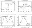
Unemployment in Europe and the United States.
In Europe, there is a neat regime shift, placed in 1980 by our Kernel density analysis, which shifts the regime mean upward from 2 .5% to 9.7%. In contrast, the U.S. analysis reveals a unique regime, only altered at the beginning of the 1980s by what seems to have been a one-off shock.9
The country-specific analysis is presented in Raurich, Sala, and Sorolla (2004), where the Kernel density analysis displayed in Figure 3 underlies the permanent regime changes plotted in Figure 2. The main conclusion is that all countries experienced regime shifts in their unemployment series.
With respect to the aggregate capital stock series for Europe, there is no long time-series directly provided by the OECD. Thus, we need to aggregate the series corresponding to the pool of countries under consideration, which involves two important requirements: first, to establish an accurate criterion to assign country weights; second, to avoid any noise derived from exchange rate fluctuations, given that the capital stock series are expressed in national currencies. The connection between capital stock and output point at GDP as the relevant measure to weight the individual capital stock series. Moreover, GDP series are generally available since the 1960s, thus allowing the computation of a yearly weight. To reach the second criterion, we use a series of real GDP in Purchasing Power Parities. Since we are not interested in the European levels of the capital stock, but on its growth rate, what we finally construct is an aggregate series of the growth rate.10
For Austria, Belgium, Denmark, Germany, and Italy, we have data on capital stock since 1960 (on the growth rate since 1961). Nevertheless, the growth rate of the aggregate capital stock series starts in 1963 because since 1962 we also have data for France and the United Kingdom, and since 1963 for Spain, all countries with substantial weight in the EU. The rest of the countries are progressively taken into account, the weights being amended correspondingly: data for Sweden start in 1965, for the Netherlands in 1968 and for Finland in 1969.
With the aggregate European and U.S. series, we conduct a Kernel density analysis and obtain the results displayed in Figure 2. In Figure 2c, a first regime is identified for Europe, lasting from 1963 to 1974, and having a mean capital stock growth rate of 4.9%. The second one starts in 1975 and lasts up to 1999, with a regime mean of 2.7%.11
Again, we present the country-specific analysis in Raurich, Sala, and Sorolla (2004), where the Kernel density analysis displayed in Figure 5 underlies the permanent regime changes plotted in Figure 4. In eight out of eleven countries two regimes are identified. Two of the exceptions are Finland and Netherlands, where only one regime is identified because of the lack of data in the 1960s (the series start in 1970 and 1969, respectively), which prevents the Kernel density analysis to consider the few data points with high values as a separate regime. It is important to note that all the regime changes take place in the mid-1970s, when the unemployment rates in these countries started to rise sharply [see Table 1 in Raurich, Sala, and Sorolla (2004)].

Capital stock growth in Europe and the United States.

Beyond this quantitative analysis, the general picture that emerges is the following. In Europe there is a permanent shift, which is expressed as an upward unemployment regime shift of 7.2 percentage points, that our analysis relates with the 2.2 percentage points reduction in the mean growth rate of capital stock. On the contrary, there is no such a permanent shift in the U.S. unemployment and capital stock growth series. The appropriateness of a multiple equilibria model for Europe, assigning a relevant role to capital formation, seems clear.
Finally, let's turn our attention to the path of the direct tax rates. In Raurich, Sala, and Sorolla (2004) the trajectory of the direct tax rates (as percentage of GDP) is related to economic growth. In particular, in all European countries with the sole exception of the United Kingdom, it can be shown that during the high regime (in the 1960s and first 1970s) the value of the tax rate was low, whereas it was high during the low regime (in the 1980s and 1990s).
As stated earlier, we interpret that a negative relationship between economic growth and the direct tax rate corresponds to a scenario of endogenous tax rates, whereas the lack of relation between these two series corresponds to a scenario of exogenous tax rates. Table 1 presents the estimates of the correlation between the direct tax rate and the growth rate taking 3-years means, which is significant in the European countries (between 5% and 25% in the Netherlands, Sweden, and Finland, but at 5% in the rest of the countries) with the exception of the United Kingdom,12
We would like to draw attention on the fact that the United Kingdom is the sole European country without a regime mean shift in the capital stock growth rates, at the same time that the pattern of its fiscal policy differs from the rest of the European countries.
These results consist on a very simple regression of the sort of the ones presented in Fatás and Mihov (2001), which take the following form: zt=α+βΔyt+νt, where zt is the fiscal variable and yt is GDP. Following Blanchard and Wolfers's (2000) and Phelps and Zoega's (2001) methodology, we take 3-years means to have a closer approximation to the structural relation between direct taxes and economic growth. Table 1 presents the estimated β for the European countries and the US.
It seems, thus, that there is a different fiscal policy pattern in Europe and the United States, which leads us to think that the fiscal policy, mainly the pattern of the direct tax rates, may be a relevant factor underlying these two areas' different economic performance.14
This is taken into account in the theoretical model presented in Section 3.THE ECONOMY
In order to provide an explanation of the empirical regularities just described, in this section we develop a simple one sector endogenous growth model with labor market frictions.
Labor Market: The Firms and Unions' Problem
The technology is described by the following aggregate production function:

where Y(t) is the gross domestic product (GDP), K(t) is the aggregate stock of capital, L(t) is the number of employed workers, and
is a production externality accruing from the average capital stock per employee in the economy.15
This externality is justified by Arrow (1962) as a result of a learning by doing process.
Assume that there is a large number of price-taker firms, implying that they do not take externalities into account when maximizing profits. Profit maximization implies that the interest rate is

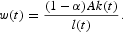
and the wage is

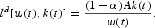
The latter equation implicitly defines the labor demand
Close the model of the labor market by assuming a simple model of firm-level wage setting, where a large number of unions set the wage to maximize:

where ws(t) is the reference wage, τ(t) is the direct tax rate and γ>0 provides a measure of the wage gap weight in the unions' objective function. When setting the wage, unions take into account the change in the amount of labor (i.e., in the firm's labor demand) but, because there is a large number of unions, the externality is not taken into account, nor the future effects on the reference wage. Thus, the solution of the unions' maximization problem is the following wage equation:
The reference wage is a controversial variable in the literature. On the one hand, in wage bargaining models it has been typically identified as an external income that workers obtain when becoming unemployed. According to this, the reference wage coincides with the average labor income [see Chapter 2, page 101, of Layard et al. (1991)]. On the other hand, Blanchard and Katz (1999) and Blanchard and Wolfers (2000) argue that the reference wage also depends on unemployment benefits, past wages, and Social Security benefits, among other variables. When the reference wage depends on past wages, there is wage inertia, as follows from (3). In that case, the reference wage is a state variable that can be interpreted as a habit stock on the average labor income because the unions' objective function depends on current wages relative to this reference level. As our aim is to emphasize the effect of wage inertia, we follow the simplifying assumption of de la Croix and Collard (2000) and assume that the reference wage is an external stock of habits that only depends on past average labor income.16
Given that unions do not consider the effects of current wages on the future reference wage, the latter is interpreted as an external habit in the unions objective function.
where ws(0) is the initial value of the reference wage, x(t) is the workers' average labor income and θ>0 provides a measure of the wage adjustment rate. Note that the higher θ, the lower is the weight of the past average labor income in determining the reference wage (and the lower is the wage inertia). Actually, if θ diverges to infinite, the reference wage coincides with the current average income, thereby excluding wage inertia. In this way, our formulation of habits includes the approach of Layard et al. (1991), in which the reference wage coincides with the current average income, as a limiting case.
The law of motion of the reference wage is obtained by differentiating (4) with respect to time
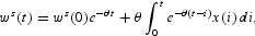
where the average labor income is assumed to be

with λ∈(0, 1), j>0, λ[1−τ(t)]w(t) being the unemployment benefits, jw(t) a wage tax,17
In our model, these taxes amount to any wage tax different from the income tax. As an example, consider Social Security contributions. Footnote 25 gives further details.
Because the current average labor income is proportional to the wage and, hence, to per capita GDP, the wage set by the unions rises with economic growth. In Section 4, we show that in the absence of wage inertia, the rise in labor demand as a result of economic growth fully translates into wage increases preventing employment growth. In contrast, when there is wage inertia, labor demand increases do not fully translate into higher wages and hence economic growth causes employment to rise. Because sustained growth implies permanent labor demand growth, wage inertia limits wage adjustments even in the long run, implying a long-run positive relation between economic growth and employment.
Consumers
Assume that there is a unique infinitely lived dynasty in the economy. Let N(t) be the number of members of this dynasty that inelastically supply one unit of labor so that the aggregate labor supply is equal to N(t) and coincides with the size of the population. This dynasty maximizes the discounted sum of the utility of each member
subject to the per capita budget constraint18
Observe that the revenues of the dynasty accrue from capital income and average labor income, which is introduced due to the assumption of a unique dynasty. These revenues should be modified if considering several dynasties with different labor incomes, but this heterogeneity would not modify the results of the paper.

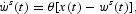
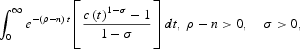
where c(t) and k(t) are, respectively, the consumption and capital stock of each member in the economy, ρ>0 is the subjective discount rate, σ>0 is the inverse of the intertemporal elasticity of substitution, n>0 is the constant population growth rate, and δ>0 is the constant depreciation rate.
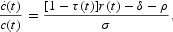
The solution to the dynasty maximization problem is characterized by the growth rate of consumption per capita
and the transversality condition

Government
Assume that the government follows a balanced budget rule, so that its budget constraint is given by the following equation:

Government revenues accruing from taxes are used to finance nonproductive government spending, G(t), and unemployment benefits. We distinguish two tax rates: (i) a direct tax on income, τ(t), that deters growth and employment, as follows from (3) and (7); and (ii) a nondistortionary tax, j, not affecting agents' decisions on employment. The aim of introducing this nondistortionary tax is twofold. First, by using this tax, the government budget constraint can be calibrated using actual data on direct tax rates and government spending. Second, it allows the government to finance part of its spending without deterring employment.
Using (1) and (2), the government budget constraint can be rewritten as follows:
where
is the fraction of GDP devoted to government spending.
We consider two different fiscal policies. First, assume that τ(t)=τ is constant and exogenous. In this case, the government sets the path of government spending to balance its budget constraint. This path is the following function of the employment rate:
Note that
as we assume that λ(1−τ)>j. Thus, government spending exhibits a procyclical path. However, total public disbursements, defined as the sum of government spending and unemployment benefits, follow a countercyclical path because of the countercyclical behavior of unemployment benefits.
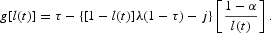
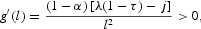
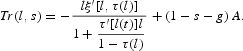
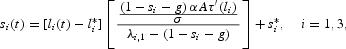
As a second fiscal policy, assume that g(t)=g is constant and exogenous, and the government sets the value of the direct tax rate to balance its budget constraint in each period. In that case, the path of the direct tax rate is endogenous and it is determined by the government budget constraint as the following function of the employment rate:
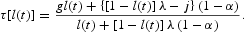
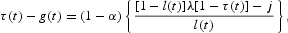
Note that
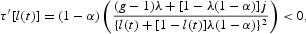
as λ(1−τ)>j implies that (g−1)λ+[1−λ(1−α)]j<0. The fact that τ′[l(t)]<0 implies that the endogenous tax rate follows a countercyclical path. In this case, total public disbursements also follow a countercyclical path because of the unemployment benefits effect.
These fiscal policies assume that the government balances its budget constraint in each period despite, as shown by the data, governments do not always proceed in this way and run deficits during recessions. Moreover, by increasing public deficits, governments can keep direct tax rates constant which, as shown in next section, implies a unique equilibrium path in our model. Nevertheless, the path of the direct tax rates in most European economies is not constant and, like public deficits, exhibit a countercyclical behavior (see Table 1). This suggests that the rise in total public disbursements during recessions are financed via both direct taxes and public deficits. When the government focuses mainly on public deficit, the rise in direct taxes will be too small to cause a strong complementarity between employment and saving decisions that explains hysteresis. In contrast, when direct taxes are mainly used, their rise during recessions may be large enough to explain hysteresis even if the government runs public deficits. Therefore, the relevant question is if the increases in the direct tax rates displayed by the data cause a sufficiently strong complementarity to explain hysteresis. Section 5 shows that, in case of hysteresis, the rise in direct taxes implied by the model is similar to the rise in these taxes occurred in several European economies (see Table 3 as an example). Thus, according to our model, the rise in direct taxes is central to explain hysteresis. As our aim is to show the economic consequences of rising direct taxes during recessions, in Section 5 we make the simplifying assumption that the government follows a balanced budget rule.19
In fact, the result of the paper would hold even if the government does not run a balanced budget rule, provided the direct tax rates are endogenous and rise strongly during recessions.
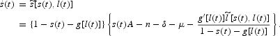
Equilibrium: The Employment and Savings Rate
To characterize the equilibrium path of the employment and savings rates, we use the resource constraint and the equations characterizing the labor market and the consumption growth rate.
Let N(t) be the aggregate labor supply, and let y(t) and k(t) be the output and capital stock per capita, respectively, satisfying y(t)=Y(t)/N(t) and k(t)=K(t)/N(t). From now on, we impose a symmetric equilibrium condition, so that d(t)=k(t)/l(t), where l(t)=L(t)/N(t) is the employment rate. Then, along a symmetric equilibrium, the per capita production function is

and the factors payments are:

and
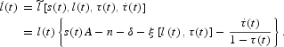
From (12), we obtain the employment rate20
Note that, because of the assumptions on the production function, per capita GDP does not depend on the number of employees, so that there are no scale effects. However, as shown in (13), the employment rate depends on capital stock.
Note that capital stock growth shifts the labor demand, which enhances the employment rate provided there is wage inertia. Note also that there is an initial condition on ws(0), as this variable is determined by past average labor income. Moreover, ws(0) determines the initial wage that is set by the unions, w(0). Finally, given the initial levels of wage and capital stock, the initial employment rate is obtained from the equilibrium labor demand l(0)=ld[w(0), k(0)]. Thus, with wage inertia, the employment rate is a state variable whose transition is driven by the degree of wage inertia.
To obtain the path of the employment growth rate, combine (3), (5) and (6) to get

Log-differentiate (3) with respect to time
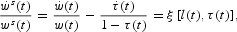
where ξ[l(t), τ(t)] is the growth rate of the after tax wage. Differentiate (13) with respect to time,

and combine it with (14) to obtain the employment growth rate
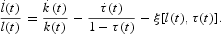
The time-path of the employment rate depends on the difference between two growth rates: the capital stock one and the one of wages before taxes. As (13) shows, capital stock growth drives labor demand growth, whereas wage growth provides a measure of the corresponding rise in the labor cost. Thus, (15) implies that the employment rate grows when the rise in labor demand is larger than the rise in the unit cost of labor.
To characterize the equilibrium path of employment, we must obtain the growth of the stock of capital. To this end, use the resource constraint

where S(t) are the savings of the economy that correspond to gross investment. Let
be the savings rate and rewrite the resource constraint as
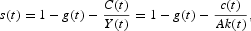
to obtain
Because in this closed economy savings coincide with gross investment, the resource constraint can be rewritten as

which can again be rewritten in per capita terms as follows

The growth of the per capita stock of capital is then
which, by using (16), becomes
Combine (15) and (17) to obtain the differential equation that drives the equilibrium path of the employment rate
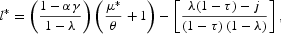
Finally, to obtain the equation that drives the path of the savings rate and summarizes the consumers' behavior, differentiate (16) with respect to time and get
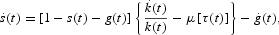
where
is the growth of per capita consumption along a symmetric equilibrium path, which is obtained from combining (11) and (7)
Combine (19) with (17) and (20), to obtain a differential equation that drives the equilibrium path of the savings rate
Observe that the equations characterizing the equilibrium depend on the nature of the fiscal policy (i.e., the tax rate being endogenous or exogenous). This distinction is important because we associate economies exhibiting acyclical tax rates (like the U.S. one) with the scenario of exogenous taxes, and economies exhibiting countercyclical taxes (like most of the European ones) with the scenario of endogenous taxes. Next we describe the equilibrium path of an economy with exogenous tax rates (Section 4) and endogenous tax rates (Section 5).
THE EQUILIBRIUM WHEN TAX RATES ARE EXOGENOUS
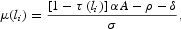
Assume that the tax rate is exogenous and constant, so that τ(t)=τ and hence
As a consequence, (18) simplifies to

and, by using (9), (21) can be rewritten as
DEFINITION 4.1. Given {l0; τ}, an equilibrium with exogenous tax rates is defined by
such that solves (9), (22), and (23), satisfies the transversality condition (8) and the following constraints: l(t)∈[0, 1], s(t)∈[0, 1] and g(t)∈[0, 1], for all t≥0.
To characterize the path of the dynamic equilibrium, first obtain the Balanced Growth Path (BGP), which is defined as a path along which l(t) and s(t) remain constant, and consumption, capital and GDP grow at the constant growth rate μ. By using
and
it is straightforward to show that the employment rate along a BGP must satisfy the following equation:

Thus, along a BGP, the long-run economic growth rate coincides with the growth rate of wages. In this simple model, this growth rate is equal to the long run growth rates of capital and, as follows from (13), of the labor demand. Thus, the employment rate attains a BGP when the growth rates of labor demand and wages coincide. In the absence of wage inertia, these two growth rates would be always equal and there would be no transition as in a standard Ak growth model. Therefore, the assumptions made on wage inertia drive the transition.
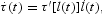
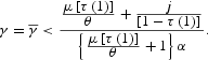
It can be shown that Q(l)=0 has a unique root, which is the unique BGP of the economy if it belongs to the close interval [0, 1], and if the corresponding savings rate and fraction of GDP devoted to government spending also belong to this interval. The BGP value of the employment rate is
where the long-run growth rate, obtained from (20), is

and the long-run savings rate, obtained from
is

We assume that μ*>0.
The acyclical behavior of the direct tax rate in the United States can be associated with this scenario of exogenous and constant tax rates. In Table 2 this version of the model is used to characterize the U.S. economy in the long run, which is taken as the benchmark economy with exogenous taxes. Table 2 also quantifies the effect of some parameter increases.

Note that when there is wage inertia (i.e., when θ does not diverge to infinite), economic growth increases the long run employment rate. Thus, in this model, a permanent decrease in TFP (A in the model) reduces the long-run growth and employment rates when there is wage inertia. To obtain the short-run effects, let us consider the transitional dynamics.
PROPOSITION 4.1. The BGP is saddle path stable and, hence, the path of the dynamic equilibrium is locally unique.
Proof. See Appendix.
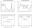
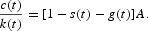
Figure 3 displays the phase diagram of this economy,21
See the Appendix for a discussion on the construction of this phase diagram and the characterization of the policy function.

Phase diagram of the economy with exogenous tax rates.
To see the effects of a shock, consider a permanent downturn in TFP (a decrease in A in the model). By using the phase lines provided in the appendix, Figure 4 displays the transition induced by this reduction, which initially causes both a substitution and a wealth effect. In Figure 4, it is assumed that the negative wealth effect dominates and hence there is an initial increase in the savings rate. Furthermore, the decrease in TFP deters growth that, as wage inertia prevents wage adjustment, causes a decline in the employment rate. This generates a further negative wealth effect that explains the rise in the savings rate during the transition. Note that the transition in the employment rate is explained by wage inertia. Actually, in the absence of wage inertia, the reduction in economic growth would be fully translated into a reduction in the wage and no effect on the employment rate would occur.

The dynamic effects of a reduction in TFP in an economywith exogenous tax rates.
As there is a unique BGP, the effects of a temporary shock are transitory. We conclude that the equilibrium does not exhibit hysteresis, which means that this model with exogenous tax rates fits the U.S. experience, but cannot explain the hysteretic behavior of unemployment in Europe.
THE EQUILIBRIUM WHEN TAX RATES ARE ENDOGENOUS
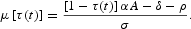
Assume now that public spending as a fraction of GDP is constant, that is, g(t)=g, and the government balances its budget constraint by setting endogenously direct taxes. From (10), it follows that τ(t)=τ[l(t)] and thus
which can be used to rewrite (18) as
and (21) as

DEFINITION 5.1. Given {l0; g}, an equilibrium with endogenous tax rates is characterized by
such that solves equations (10), (25), and (26), and satisfies (8) and the following constraints: l(t)∈[0, 1], s(t)∈[0, 1], and τ(t)∈[0, 1] for all t≥0.
The BGP of this economy is obtained when
and
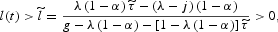
which yield the following equation characterizing the employment rate along a BGP:

where τ(l) is obtained from (10). Again, along a BGP the growth rates of labor demand and wages are equal. However, when the tax rates are endogenous, Q(l) is a third order polynomial that may have three real roots within the relevant domain, that is, the close interval [0, 1].22
The functional form of Q(l) is shown in the proof of Proposition 5.2, in the Appendix.

These multiple BGPs arise because the endogenous tax rates generate a complementarity between the employment and the savings decisions, making agents' expectations to be self-fulfilling. To explain this complementarity, assume that agents coordinate into an expectations of high net interest rate. If agents are willing to substitute intertemporally consumption, the savings rate will be large and thus the growth rates of capital stock and labor demand will also be large. When there is wage inertia, the latter implies a high value of the employment rate, which, given its impact on economic activity, causes large government revenues and low expenditures. Obviously, the endogenous direct tax rate is low and hence the net of taxes interest rate is large in equilibrium. Thus, endogenous tax rates make agents' expectations hold in equilibrium, which explains the existence of an equilibrium path corresponding to a regime of high economic activity. The same argument applies to explain the equilibrium path of a low regime.
Denoting the BGPs by l1, l2, and l3, assume, without loss of generality, that l1<l2<l3. Along each BGP, the tax rate is obtained from (10) as a function of the employment rate, τ(li), for i=1, 2, 3. As τ′(l)<0, the long-run tax rates satisfy the following relations: τ(l1)>τ(l2)>τ(l3). From (20), it follows that the long-run economic growth rate is
which is negatively related to the tax rate implying that, along the BGP, μ(l1)<μ(l2)<μ(l3). Finally, the long run savings rate is obtained from

Because the savings rate is positively related with economic growth, the following relations hold: s(l1)<s(l2)<s(l3). Thus, it follows that BGP 1 [[i.e., l1, τ(l1), μ(l1), s(l1)] corresponds to a regime of low economic activity and high tax rates, whereas BGP 3 [i.e., l3, τ(l3), μ(l3), s(l3)] corresponds to a regime of high economic activity and low tax rates.
The countercyclical behavior of the direct tax rate in Spain is associated with our scenario of endogenous tax rates and, as Table 3 shows, the model is able to replicate fairly well the two regimes of the Spanish economy. Because BGP 2 is unstable, we identify BGP 1 with the low regime of the Spanish economy and BGP 3 with the high regime.
PROPOSITION 5.1. BGPs 1 and 3 exhibit saddle path stability, whereas BGP 2 may be either unstable or locally stable.
Proof. See Appendix.
Further numerical examples beyond the one in Table 3 show that the instability of BGP 2 is a robust result. Thus, hysteresis, which we identify with the shift between equilibrium paths converging to different BGPs, may only arise when there are three BGPs. In this case, agents can coordinate into an equilibrium path that converges to BGP 1 or into another one that converges to BGP 3. Proposition 5.2 provides sufficient conditions that prevent the existence of three BGPs, which help to understand how savings decisions, the fiscal policy and labor market institutions interact to explain hysteresis.
PROPOSITION 5.2. If
or
then at most two BGPs exist.
Proof. See Appendix.
The results in Proposition 5.2 imply that the existence of three BGPs requires labor market rigidities in the form of: (i) wage inertia, which ensures the positive effect of economic growth on employment; and (ii) a sufficiently large wage gap weight in the unions' objective function. Second, the intertemporal elasticity of substitution must be sufficiently large, since the complementarity requires the savings rate to increase with the interest rate (note, however, that multiple BGPs arise under plausible values of the intertemporal elasticity of substitution, as shown in the example of Table 3).23
Ogaki and Reinhart (1998) provide estimates of the intertemporal elasticity of substitution between 0.32 and 0.45. The value of this elasticity in Table 3 is 0.28, which is below these estimates.
Concerning the first condition, the proof of Proposition 5.2 shows that, if the nondistortionary tax is not sufficiently large, economic growth in the long run will be negative in the low regime, which is not sustainable as an equilibrium. To see this note that, since by equation (3) wages are a markup over the reference wage, it follows that wages before taxes increase with the direct tax rate; hence, when agents coordinate in the low equilibrium (along which the tax rates rise), wages also increase along the transition and make the employment rate decrease, rising in turn the direct tax rate and reinforcing the negative effect on employment. When the only tax is the income tax, this transition diverges toward a zero employment rate and a negative growth rate. The introduction of a nondistortionary tax making the reference wage to decrease with the direct tax rate prevents this to happen,24
In fact, as follows from (3.6) any additional wage tax, such as j, makes the wage net of direct taxes and the average labor income be nonproportional. When this happens, the direct tax rate reduces the reference wage growth and, hence, decreases wages.
The tax j can be identified as a Social Security tax because it is proportional to the wage. The assumptions on fiscal policy imply that i) this tax is not taken into account by the unions when setting the wage, which means that this tax does not affect the markup and, hence, it is not distortionary; and ii) both unemployed and employed workers pay this tax. It can be shown that both assumptions can be removed and yet the reference wage will decrease with the direct tax rate. Thus, our particular assumptions on j are introduced just for the sake of simplicity.
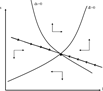
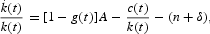
The intuition behind the second condition can be clearly seen through the long-run Laffer curve. To construct this curve, note that along the BGP, both the exogenous and the endogenous tax rate economies are characterized by the same two equations: the government budget constraint and the equality between the growth rates of wages and economic growth. In (24), we have shown that this equality holds when l*=l*(τ) so that, by using the government budget constraint (9), we obtain

which is the long-run Laffer curve displayed in Figure 5, relating the tax rate with the fraction of GDP devoted to government spending. Note that in the exogenous tax rate economy, given a value of the tax rate, we obtain a unique value of government spending and, thus, a unique BGP. In contrast, in the economy with endogenous tax rates, different tax rates may finance a given value of government spending. These different tax rates are the different BGPs, corresponding to a high tax rate and low economic activity regime (the wrong side of the Laffer curve), and to a low tax rate and high economic activity regime (the right side of the Laffer curve). Figure 5 shows that there are three BGPs only when government spending belongs to a given interval. When government spending is too large, it can only be financed by means of a large tax rate; when too low, it can only be financed by means of a low tax rate.

Long-run Laffer Curve.
The transitional dynamics along these equilibrium paths, that converge to BGPs belonging to the same Laffer curve, are driven by agents' expectations on the tax rate. If they expect tax rates to be large (small), they expect the net interest rate to be low (large) and, hence, the initial savings and growth rate will be low (large). This implies that the equilibrium converges to a low (high) economic activity regime, where tax rates are large (low) in equilibrium. In this way, agents' expectations are fulfilled and agents may coordinate into any equilibrium. In contrast, when tax rates are exogenous, the equilibrium is unique because the government selects the equilibrium path by setting the value of the tax rate.
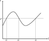
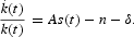
The transitional dynamics with endogenous taxes are displayed in Figure 6, picturing the phase diagram when there are three BGPs. Note that, given an initial value of the employment rate, agents may coordinate, by means of their savings decisions, into an equilibrium path driving toward the high regime (BGP 3) or into an equilibrium path driving towards the low regime (BGP 1).

Phase diagram of the economy with endogenous tax rates.
As shown in the Appendix, the policy functions driving toward BGPs 1 and 3 have a positive slope when tax rates are endogenous. Thus, if the economy converges to one of these BGPs, the equilibrium exhibits a positive relationship between the employment and the savings rate, which is in stark contrast with the negative relationship obtained when tax rates are exogenous. The reason is that an increase in the employment rate implies lower government expenditures and higher revenues. As a consequence, the endogenous tax rate decreases with the employment rate, thereby increasing the net of taxes interest rate, which rises the savings rate.
With three BGPs, a temporary shock, such as a reduction in TFP, may make agents coordinate into another equilibrium path and thus have permanent effects and generate hysteresis. Figure 7 displays the phase diagram when we assume that the equilibrium is initially in BGP 3 and there is a TFP shock (a reduction in A) that opens two possibilities of coordination giving rise to two different equilibrium paths. In one of them, agents choose an initial small reduction in the savings rate that makes the economy go back to BGP 3. In the other one, agents choose a large initial reduction in the savings rate, which places the economy in the policy function converging towards BGP 1, that is, the equilibrium converges towards the wrong side of the Laffer curve, where the tax rate is large and the interest rate is low.

The dynamic effects of a reduction in TFP in an economywith endogenous tax rates.
Observe that the long-run effects of a reduction in TFP depend on the initial jump in the savings rate that, in turn, depends on agents' expectations. Interestingly, when these expectations make agents coordinate into another equilibrium path, temporary shocks have permanent effects and cause hysteresis. To understand why, note that the reduction in TFP has a direct negative effect in the gross interest rate that makes agents be willing to reduce savings. However, the overall effect on the savings rate depends on the net interest rate, in turn depending on agents' expectations. In particular, if agents coordinate into an expectation of low tax rates, they will expect a small decrease of the net interest rate. As a consequence, they will choose a tiny initial reduction in the savings rate implying a small reduction in economic growth and a small decline in the long run employment rate. In this case, the equilibrium converges to the BGP with high activity. Because employment is large, government disbursements as a fraction of GDP are low, the required equilibrium tax rate is thus small and expectations are fulfilled in equilibrium. However, agents also may coordinate into an expectation of high tax rates, with agents expecting a large reduction in the net interest rate and thereby choosing a large decrease in the savings rate that causes a large decline in economic growth and, hence, in the long-run employment rate. Therefore, the equilibrium converges to the BGP with low economic activity and high tax rates. In this equilibrium, expectations are fulfilled again, but now a temporary reduction in TFP has permanent effects.
To conclude, according to our model, the different economic performance of the United States and the European countries after the temporary shocks of the 1970s can be explained by a different response in terms of fiscal policies. In the United States, direct tax rates were kept constant, and employment and growth suffered a temporary decline. In Europe, direct tax rates increased and employment and growth suffered a persistent decline. The model explains this persistent decline as a result of a coordination into another equilibrium path.
CONCLUDING REMARKS
We have used a growth model with a noncompetitive labor market to show that endogenous tax rates generate complementarities between employment and capital yielding the possibility of multiple equilibria. With multiple equilibria, the equilibrium path is the result of a coordination among equilibria with high tax rates and low employment and savings rates; and equilibria with low tax rates and high economic activity. These equilibrium paths converge to different long-run equilibria that belong to opposite sides of the same Laffer curve.
When tax rates are endogenous, agents may coordinate on either side of the Laffer curve. This coordination failure causes economic instability and, furthermore, agents may coordinate into an equilibrium path that converges to the wrong side of the Laffer curve (the low regime). In contrast, when tax rates are exogenous, the government selects the equilibrium path setting the value of the tax rate. In this way, the government prevents economic instability and may place the economy in an equilibrium path that converges to the right side of the Laffer curve. Thus, according to this model, those fiscal policies not using the direct tax rate to balance the government budget constraint are a superior fiscal policy.
The model also nests an interpretation of the different performance of the U.S. and the European economies in the aftermath of temporary shocks such as those occurred in the 1970s. In particular, we find a correspondence between the acyclical behavior displayed by the direct tax rates in the United States with our scenario of exogenous tax rates, and their countercyclical behavior in most of the European countries with our scenario of endogenous tax rates. In response to a temporary reduction in TFP, in the first case the model implies a temporary decline in the employment, savings and growth rates, which matches well with the U.S. experience. In the second case, the model predicts the possibility of hysteresis, which also fits the extremely persistent reduction in the path of employment, growth and saving rates occurred in Europe. The model explains this permanent reduction as a coordination of agents into an equilibrium with high tax rates and low employment and savings rates.
APPENDIX
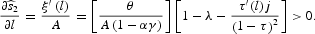
Proof of Proposition 4.1. The BGP exhibits saddle path stability when the determinant of the Jacobian matrix formed by (23) and (22)
is negative

Phase diagram of the economy with exogenous tax rates. Denote by
the phase line associated to
. The slope around the BGP is given by
which can be either positive or negative. If
then the phase line is

and

Figure 3 displays the phase diagram when
Note that the slope of the policy function is negative. When
,
and the slope of the policy function is also negative. To see this, use the Jacobian Matrix to obtain the equation of the policy function relating s(t) with l(t)

where λ1<0 is the stable eigenvalue. It can be shown that |J+lξ′(l)I|<0, where I is the identity matrix. This inequality implies that λ1<−lξ′(l), and hence the policy function has a negative slope.
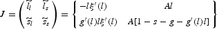
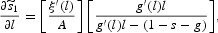
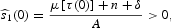
Proof of Proposition 5.1. To discuss the stability of each BGP, obtain the elements of the Jacobian matrix formed by equations (26) and (25)

and find its determinant
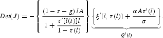
By using (10), obtain

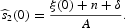
This inequality implies that the sign of the determinant is the opposite of the sign of the slope of the function Q(l). As Q(0)=−[θ+μ(0)]<0, it must be that Q′(l1)>0, Q′(l2)<0 and Q′(l3)>0. It follows that the determinant is negative at the BGPs 1 and 3, and positive at BGP 2. In BGP 2, stability depends on the sign of the trace, which is given by
BGP 2 is unstable when
and it is locally stable when
Proof of Proposition 5.2. The proof follows from Q(l)=0 which, by using (10), can be rewritten as

Note first that if either
or θ→∞, then a root of Q(l)=0 is
which implies that there are at most two BGPs. Next, given that Q(0)<0, it follows that there are at most two BGPs when Q(1)<0. This happens when
Note also that

if
where
and
are the roots of Q(1)=0. By using (9), get Q(1)<0 when
where
and
Thus, when
there are two BGPs at most.
Finally, note that μ[τ(l)]>0 when
which requires that
as follows from (10) and by noticing that the denominator of
is negative. Next, it can be shown that ∂Q(l)/∂j<0, which means that ∂l1/∂j>0. Moreover, l1→0 as j→0, implying that there exists a value of j,
such that if
then
and there are, at most, two BGPs with positive growth rates.
Phase diagram of the equilibrium with endogenous tax rates. The phase lines are the following. If

If
,

Note that

and
Note also that
and
Therefore, Q(0)<0 implies that ξ(0)<μ(0) so that
. Thus, s1(l) and s2(l) are increasing and
Using these properties of the phase lines, we can construct the phase diagram displayed in Figure 6.
By using the Jacobian matrix, we obtain the equation of the policy function that converges to either BGP 1 or 3
where λi,1 is the stable root associated to BGP 1 or 3. Note that the slope of this equation is positive when τ′(li)<0.
We thank Jaime Alonso-Carrera, José E. Boscá, Rafael Doménech, Tim Kehoe, José Victor Rios-Rull, Dennis J. Snower; seminar participants in Vigo, Mallorca, Barcelona, Valencia, EALE 2004 (Lisboa), and the Terceras Jornadas Béticas de Macroeconomía Dinámica (Málaga) for helpful comments. We are grateful to the Spanish Ministry of Education for financial support through grants SEC2003-00306 and SEC2003-7928, and to the Generalitat de Catalunya through grant SGR2001-164.