INTRODUCTION
The growth effect of money supply is one of the central research concerns in the money and growth literature. In particular, if the economy allows endogenous growth and if money is not supernuetral, then monetary policy may have profound effects on the long-term behavior of the economy. Most of the existing studies on money and endogenous growth have concluded that in economies with infinitely lived agents, a higher money growth depresses the long-run growth rate of the economy. The literature has demonstrated that this conclusion holds in a wide variety of monetary endogenous growth models: see, for example, Howitt (1990), De Gregorio (1993), Jones and Manuelli (1995), Marquis and Reffitt (1991 and 1995), Pecorino (1995), and Mino (1997). The mechanism that generates the negative relationship between monetary and real growth in the infinitely lived, representative agent economy has an intuitive appeal: a higher growth of money supply raises the inflation tax on the rate of returns to physical (and human) capital, so that investment will be reduced to yield a lower growth rate of the economy.1
In overlapping generations models with endogenous growth, however, inflation and growth may be positively correlated: see, for example, Mino and Shibata (2000). Itaya and Mino (2003) and Jha et al. (2002) examine endogenous monetary growth models based on transactions cost approach to money.
The purpose of this paper is to reexamine the fundamental observation mentioned above. We add two extensions to the conventional models employed by the existing studies on money and endogenous growth. First, the model economy examined in this paper is subject to increasing returns to scale. Second, we use a more general utility function in which consumption and leisure can be nonseparable. In the real business cycle studies, it has been known that both production technology and preference structure are crucial for policy impacts as well as for the dynamic behavior of the economy. We demonstrate that this conclusion can be confirmed in the monetary growth models as well. Namely, both the production technology and the preference structure may play essential roles in determining the growth effect of money supply. The analytical framework of our discussion is based on the model examined by Benhabib and Farmer (1994) that has been frequently used to discuss sunspot-driven business cycles. We introduce money into an endogenous growth version of the base model via a cash-in-advance constraint. Because the model allows labor-leisure choice, money is not superneutral in the long-run equilibrium, even though the cash-in-advance constraint applies to consumption alone.2
It is to be noted that Fukuda (1996) also introduces money into the Benhabib and Farmer model with a separable utility function. Because we use a more general preference structure, our discussion involves Fukuda's main conclusions as special cases. Because Fukuda (1996) mainly focuses on the case of exogenous growth in which long-term growth cannot be sustained, our study overlaps a part of his paper that treats the case of endogenous growth.
Our main finding is that the growth effect of money supply hinges on the degree of increasing returns characterizing production technology as well as on the elasticity of intertemporal substitution in consumption. More specifically, if the elasticity of intertermporal substitution in consumption is lower than one and if production externalities are relatively small, we obtain the conventional results, that is, the balanced-growth path is uniquely given and a rise in money growth reduces the long-term growth rate. In contrast, if the elasticity of intertemporal substitutability is smaller than one but the degree of increasing returns is high enough, then there may exist dual balanced-growth paths. In this case an increase in money growth decreases (increases) the growth rate on the balanced-growth path with a higher (lower) growth rate. Those results are, however, reversed if the elasticity of intertemporal substitution in felicity exceeds one. Under such a preference characterization, if the degree of increasing returns is relatively small, then dual balanced-growth paths may exit. If this is the case, a rise in monetary growth increases (decreases) the long-term growth rate in the high- (low-) growth equilibrium. Moreover, if both the degree of increasing returns and the elasticity of intertemporal substitutability are high, the balanced-growth path can be unique and a higher money growth accelerates long-run growth.
In addition to the growth effect of money supply, we investigate dynamic properties of the model economy out of the balanced-growth equilibrium. We find that, as well as in the real business cycle models without money, the uniqueness of transitional path of the monetary economy heavily depends on specifications of production technology and preference structure. For example, in the presence of unique balanced-growth equilibrium, the converging equilibrium path is uniquely determined when both the degree of increasing returns and the elasticity of intertemporal substitutability are relatively small. By contrast, when either the degree of increasing returns or the elasticity of intertemporal substitution in consumption is high, a continuum of converging paths emerges around the balanced-growth equilibrium. Additionally, it is shown that if there are dual balanced-growth equilibria, one of them is determinate and the other is indeterminate. Which balanced-growth path exhibits determinacy again depends upon the specifications of technology and preferences. Based on those findings, we consider the relationship between the determinacy of equilibrium and the growth effect of money supply.
The rest of the paper is organized as follows. Section 2 sets up an analytical framework for the subsequent discussions. Sections 3 contains our main discussions. It considers the steady-state effects of a change in the money growth rate as well as the local dynamic behavior of the balanced-growth under alternative conditions on the parameter values characterizing the technology and preferences. Section 4 presents intuitive implications of our main findings. Section 5 concludes the paper.
THE ANALYTICAL FRAMEWORK
Production
In formulating the production side of the economy, we follow Benhabib and Farmer (1994). There are many identical firms whose number is normalized to one. The production technology of each firm is specified as

where y is output, k is capital and l is labor. Here,
and
respectively represent positive external effects associated with the capital and labor of the economy at large. We assume that the private technology satisfies constant returns, but the social technology involving the external effects exhibits increasing returns to scale.
The final goods and factor markets are competitive, so that the rate of return to capital, r, and the real wage rate, w, are equal to the marginal products of private capital and labor, respectively:

Because we have assumed that the total number of firms is one, it always holds that
and
in equilibrium. In this paper, we focus on the situation in which endogenous growth is sustained by capital externalities. This means that α=1, and hence the aggregate production function at the social level is

and the equilibrium levels of the return to capital and real wage rate are respectively expressed as


Households
There is no population growth and the number of households is also normalized to be one. The representative household maximizes a discounted sum ofutilities

subject to

In the above, c is consumption, a total asset, m real money balances, i the nominal interest rate and τ denotes an income transfer from the government. We assume that the government does not issue debt so that the total wealth of the household consists of capital and money holdings. In this paper, we assume that the cash-in-advance constraint is applied to consumption spending alone.
The instantaneous utility function, u(c, l), is assumed to be monotonically increasing in consumption and decreasing in labor. In what follows we use a specific form of function such that

where Λ(l) is strictly positive and it satisfies the following:

These conditions ensure that the felicity function decreases with labor and it is strictly concave in consumption and labor.
To obtain the necessary conditions for an optimum, let us define the current-value Hamiltonian function:

where λ is the costate variable of a, and μ and γ are Lagrange multipliers. If we focus on an interior solution, the necessary conditions for an optimum are given by the following:


together with the transversality condition: limt[rhard ]∞aλe−ρt=0 and the initial condition on a.
Money Growth and Market Equilibrium
Because this paper does not focus on comparison of the alternative money supply rules, we assume the simplest money supply regime. Namely, the growth rate of nominal stock of money is kept constant and the newly created money is distributed to the households as lump-sum transfers. Denoting the growth rate of money supply by θ, we see that the real money balances behave in accordance with

The government budget constraint is thus given by τ=θm.
The market equilibrium condition for the final good is

For notational simplicity, we assume that capital does not depreciate. Finally, the nominal interest rate is determined by the Fisher equation:

where π denotes the rate of inflation.
The Dynamic System
Equations (8) and (9) yield μ/λ=i. Thus using (2), (6), (7), (8), and (9) we obtain

This states that the marginal rate of substitution between labor and consumption is equal to the relative price between leisure and consumption. Notice that when the cash-in-advance constraint is effective, an additional unit of consumption needs an additional unit of real money balances so that the effective price of consumption is one plus the nominal interest rate, i, which represents an opportunity cost of money holding. Therefore, w/(1+i) expresses the real wage rate in terms of the effective price of consumption. Using (2), (3), (13), and (14), we find that the rate of inflation is expressed as

where x≡k/c,
As we focus on an interior equilibrium, it holds that c=m for all t≥0. Hence, from (11) and (15) consumption changes according to

Equations (3) and (7) yield

Logarithmic differentiation of both sides of the above equation with respect to time yields

where η(l)≡Λ′′(l)l/Λ′(l)>0. Therefore, using (1), (2), (9), (10), (12), and (16), the above expression can be rearranged as

where η(l)+1−β≠0. In addition, (1), (12), and (16) mean that behavior of x(≡k/c) is described by the following:

To sum up, (17) and (18) constitute a complete dynamic system with respect to l and x.
GROWTH EFFECT OF MONEY SUPPLY
The Balanced-Growth Equilibrium
From (17) and (18) the steady-state levels of l and x satisfy the following conditions:


The steady-state conditions shown above mean that on the balanced-growth path capital, consumption as well as real money balances grow at a common rate, while the level of employment stays constant over time. By use of (15), (19), and (20), we obtain the following equation:

If this equation has a positive solution, then there exists a steady-state value of l. In order to conduct a graphical analysis of (21), let us define the following functions:


If F(L)−G(L)=0 has a positive, feasible solution, it gives the steady-state level of l.
Because the capital share of income, a, may be about 0.3 in reality, if σ<a, we should assume that the intertemporal elasticity of consumption, 1/σ, takes an implausibly high value. Thus, in order to focus on economically plausible cases, we assume that σ>a. Inspecting the graph of G(l) function defined earlier, we can easily confirm that if σ>1(a<σ<1) and if F(l) is monotonically decreasing (increasing) for all feasible l, then F(l)−G(l)=0 has a unique positive solution. Otherwise, there may exist two solutions at most. The exact shape of F(l) cannot be determined without further specifications. Therefore, we use the following function as a typical example to obtain clear-cut results:

which is defined on l∈[0, 1]. Because 1−l represents leisure, (24) means that the instantaneous felicity of the household is expressed as the standard Cobb-Douglas function of consumption and leisure in such a way that

Note that this function fulfills the concavity conditions in (5) for σ>χ/(1+χ). Because we have assumed that σ>a, in what follows we assume that
Given this specification, we find that F(l) is written as

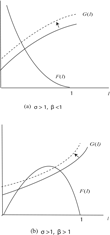
Figures 1(a) and 1(b) depict the relations between the graphs of F(l) and G(l) under σ>1. Figure 1(a) shows the case of β<1. In this situation, F(l) is monotonically decreasing and satisfies that liml→0F(l)=+∞ and F(1)=0. In addition, G(l) is a monotonically increasing function for l≥0. Thus F(l)−G(l)=0 has a unique, positive solution. Figure 1(b) assumes that σ>1 and β>1. Under these conditions, F(0)=F(1)=0 and sign F′(l)= sign
Moreover, G(l) is increasing, strictly convex and G(0)=(ρ/σ)(ρ/σ+θ+1)>0. Thus if F(l)−G(l)=0 has a solution, it involves two roots for l≥0.

Effects of a monetary expansion under σ > 1.
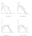
Figures 2(a) through 2(d) display the graphs of G(l) and F(l) for
In these cases, the graph of G(l) is inverse-U shaped and
where
Thus when β<1, there may exist dual steady-state levels of l if
while the steady state is uniquely determined if
: see Figures 2(a) and 2(b). In the case of β>1, as shown by Figures 2(c) and 2(d), F(l)−G(l)=0 has a unique positive solution if
while there are two solutions at most if

Effects of a monetary expansion under σ < 1.
Effects of Monetary Expansion
From (1), (12), (19), and (20) the balanced-growth rate and the steady-state rate of inflation are respectively given by


where g denotes a common, balanced-growth rate of y, k, c and m. Hence, the balanced-growth rate increases with l and the rate of inflation decreases with l. This implies that the balanced-growth path with a higher employment level attains a higher growth rate and a lower rate of inflation, while the other steady state with a lower employment yields a lower growth rate and a higher rate of inflation.
Considering the steady-state characterization displayed earlier, we can easily examine the effects of an increase in the monetary growth rate, θ, on the steady-state rates of income growth and inflation. Notice that an increase in θ yields an upward shift of the graph of G(l). Because the graph of F(l) is unaffected by a change in θ, it is easy to establish the following comparative statics results:
PROPOSITION 1. If functions F(l) and G(l) given by (22) and (23) satisfies G′(l)>F′(l) at the steady state, an increase in money growth rate depresses the balanced-growth rate. If G′(l)<F′(l) at the steady state, an increase in money growth raises the balanced-growth rate.
By using graphical analysis of G(l) and F(l) functions, we find that the negative relation between θ and l if G′(l)>F′(l) holds at the balanced-growth equilibrium. In contrast, if G′(l)<F′(l) is satisfied, the steady-state level of l (so the balanced-growth rate, g) is positively related to the money growth rate, θ. It is worth emphasizing that these graphical relations do not depend on our specification of Λ(l) function. Because the shapes of G(l) and F(l) functions are characterized by the parameters concerning preferences and technology, this proposition clearly demonstrates that the growth effect of money supply critically relies on the preference structure as well as on the production technology.
If Λ(l) function is given by (24), then in the presence of a unique balanced-growth path, a rise in the money growth rate, θ, lowers the long-term growth rate of income and raises the rate of inflation if β<1 [see Figures 1(a) and 2(a)], while it increases the growth rate of income if β>1 [see Figure 2(d)]. If σ>1 and if dual balanced-growth paths exist, then a rise in θ depresses the growth rate of income and increases the rate of inflation at the high-growth equilibrium, while it increases the growth rate of income at the low-growth equilibrium: see Figure 1(b). If
and
then the opposite results hold: see Figures 2(b) and 2(e). Table 1 summarizes these findings. In the table, High and Low respectively denote the balanced growth path (BGP) with a higher and lower growth rate. In addition,
and
.3
The definition of
states that
is relatively large if θ, ρ and σ are large and it is relatively small if A, β and α are high.

Dynamics
Next, let us examine the dynamic property of our model economy around the balanced-growth equilibrium. When we linealize the dynamic system consisting of (17) and (18) at the stationary point, the Jacobian matrix of the linearized system is given by

where l and x indicate their steady-state values. Because we treat an endogenous growth model with an Ak technology, both of the initial values of l and x (=k/c) are unpredetermined. This means that if the linearized system is completely unstable around the steady state (i.e., the stationary point is a source), the economy can always stay on the balanced growth path so that local determinacy of equilibrium is established. However, if the steady state of the dynamic system is either a saddle-point or a sink, then there exists a continuum of converging equilibria and hence local indeterminacy emerges. Keeping these facts in mind, we can show the following analytical results:
PROPOSITION 2. The balanced-growth equilibrium has a local saddlepoint property, either if η(l)+1−β>0 and F′(l)>G′(l), or if η(l)+1−β<0 and F′(l)<G′(l) at the steady state.
The proof of this proposition is shown in Appendix 1 of this paper. It is worth emphasizing that the stability property is related to the sign of η(l)+1−β, while the characterization of the steady state and the growth effect of money supply critically depend on the sign of 1−β. Therefore, if we consider both the stability and steady state characterization, we should classify the cases into β<1, 1<β<1+η(l) and β>1+η(l). Applying these results to the case of Cobb-Douglas utility given by (25) we find that local determinacy of equilibrium around the steady state may be summarized as Table 2. In the table, notation D and I, respectively, indicate determinacy and indeterminacy of BGP. Appendix 2 presents the detail on how to drive the results shown in the table.

Tables 1 and 2 demonstrate that there are various patterns of the relationship between the growth effect of money supply and determinacy of equilibrium. That is, we may have the counter-intuitive, positive relation between money growth and real growth, even if determinacy is satisfied around the balanced-growth path. At the same time, the standard negative relation between money growth and real growth can be established even in the long-run equilibrium with local indeterminacy. For example, when σ>1 and β<1, the unique balanced growth path holds local determinacy. In contrast, although there is a unique balanced-growth equilibrium, it is locally indeterminate if 1<β<1+η(l) and σ<1. However, if β exceeds 1+η(l), the long-run equilibrium becomes locally determinate. In these cases, the growth effect of money supply is negative if σ>1 and β<1, while it is positive if β>1 and σ<1.
Separable Utility
In order to emphasize the role of preference structure in our discussion, it is useful to examine a simple case of additively separable utility. Suppose that the instantaneous utility is given by

where Φ′(l)>0 and Φ′′(l)>0. It is easy to confirm that the dynamic equation of l in this case may be obtained by setting σ=1 in (17) while the behavior of x is the same as (18). Thus the complete dynamical system in the case of separable utility is given by

where η(l)≡Φ′′(l)l/Φ′(l)(>0) and the rate of inflation, π(l, x), is given by

As a result, the steady-state conditions under which
can be summarized as the following equation whose solution gives the steady state value of l:

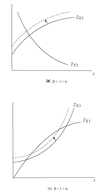
We see that the left-hand side of (30) is monotonically decreasing (resp. increasing), if η(l)+1−β>0 (resp.η(l)+1−β<0) for all l>0. Figures 3(a) and 3(b), in which
and
show the existence of the steady state level of l. As Figure 3(a) depicts, if η(l)+1−β>0, the balanced-growth equilibrium is uniquely given. If η(l)+1−β<0, then there are two steady states at most: see Figure 3(b). A typical example of Φ(l) function is

where η is a positive constant, then η(l)(=Φ′′(l)l/Φ′(l)=η) is fixed for for all l>0. This specification of disutility of labor has been frequently employed in the real business cycle literature. Because η is constant for all l>0 in this case, the global argument given above always holds.

Effects of a monetary expansion in the case of separable utility.
It is also to be noted that in the case of unique balanced-growth path, it is locally determinate. In the case of dual steady states, the BGP with a lower growth rate (i.e., a lower l) is locally determinate and that with a higher growth rate (i.e., a higher l) is locally indeterminate. The positive relation between the balanced-growth rate and the monetary expansion rate, θ, holds only at the steady state with a lower growth in the case of dual steady states. These results mean that the growth impact of money supply as well as dynamic behavior of the economy mostly depend on the production technology if the instantaneous utility function is additively separable between consumption and labor. Therefore, the relation between money growth and real growth in the case of separable utility is essentially the same as that held in the model with nonseparable utility and σ>1.
To sum up, we have shown:
PROPOSITION 3. If the utility function is given by (29) and if β<1+η(l) for all l>0, then (i) the balanced-growth equilibrium is unique and globally determinate, and (ii) a rise in money growth lowers the balanced-growth rate. If β>1+η(l) for all l>0, there may exist dual steady states at most. In the presence of dual steady states, (i) the balanced-growth equilibrium with a lower (resp, higher) growth rate is locally determinate (resp, indeterminate), and (ii) an increase in money growth decreases (resp, raises) the real growth rate in the steady state with a higher (resp, lower) growth.
DISCUSSION
The Roles of Technology and Preference
In this section we present intuitive implications of the roles of production technology and preference structure in determining the growth effect of money supply. To do so, we assume that the economy initially stays on the balanced-growth path and that there is a permanent rise in the growth rate of nominal money supply, θ.
Notice that the steady-state rate of nominal interest rate satisfies i=r+π=(σ−1)g+ρ+θ, because r=σg+ρ and π=θ−g in the balanced-growth equilibrium. First, consider the case of separable utility given by (29) As was shown, in this case the growth effect of money depends mainly on the magnitude of β. Noting that under the separable utility assumption i=ρ+θ on the balanced-growth path, we can rewrite (30) as

The left-hand side of (31) is the steady-state expression for the marginal rate of substitution between consumption and labor, while the right-hand side shows the steady-state level of real wage rate in terms of effective price.4
More precisely, the left-hand side of (31) is the marginal rate of substitution, whereas the right-hand side represents the (effective) real wage.

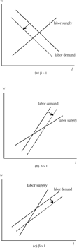
Effect of a monetary expansion on the labor demand curve.
If β>1, then the labor demand curve has a positive slope. As shown by Proposition 3, in this case there may exist two steady states and it is straightforward to confirm that the long-run labor demand curve is steeper (resp. flatter) than the labor supply curve at the steady state with a lower (resp. higher) level of l.5
The slope of the graph of the LHS in (31) is (1−a)βAlβ−1Φ′(l)+[(1−a)Alβ+ρ]Φ′′(l), and that of the RHS is (1−a)(β−1)Alβ/(1+ρ+θ). Remember that the graphs given in Figure 3 satisfy

Thus, keeping mind that
holds in the steady state, we find that if
at the intersection, the slope of the demand curve is steeper than that of the labor supply curve, and vise versa.
We should note that the growth effect of money supply in the case of separable utility essentially has the same effect of labor income taxation in the absence of cash-in-advance constraint. If there is no money and if real factor incomes are subject to distortionary taxation, the household's budget constraint is replaced with

where τk and τl denote the tax rates on capital income and labor income, respectively. Given this constraint, the first-order condition for an optimum (14) becomes

Thus the labor market equilibrium condition corresponding to (31) is modified as

Replacing 1−τl with (1+θ+ρ)−1 in this equation, we see that a rise in the rate of labor income tax, τl, yields the same growth effect as that of an increase in the money growth rate, θ. Hence, when the preference structure satisfies additive separability between consumption and labor, the inflation tax plays the role exactly analogous to that played by the labor income taxation.6
Here, we implicitly assume that the income tax is not levied on leisure.
When the utility function is not separable between consumption and labor, the nominal interest rate in the steady state is i=(σ−1)g+ρ+θ. By use of g=(1/σ)(r−ρ), we find that the relation between the long-term nominal interest rate and the steady-state level of employment is

This equation demonstrates that if σ≥1, the nominal interest rate increases with the employment level (so the balanced-growth rate) in the steady state, while it decreases with l if σ<1. In view of (32), the equality between the marginal rate of substitution and the real wage rate in the steady state given by (14) can be rewritten as

where i is given by (32). Because the case of σ≥1 yields the outcomes similar to those obtained in the model with separable utility, we examine the case of
To make an intuitive discussion clear, let us further assume that the instantaneous utility is given by (25). The left-hand side of (33) becomes
which increases with l so that the labor supply curve always has a positive slope. First, suppose that β>1. In this case a higher l increases the marginal product of labor, (1−a)Alβ−1, while it decreases the nominal interest rate given by (32). Hence, the labor demand curve represented by the right-hand side of (33) increases with l. As shown by Figure 4(c), if the labor demand curve is less steeper than the labor demand curve, a downward shift of the labor demand caused by a rise in θ reduces the steady state level of l. In contrast, if the labor demand curve is steeper than the labor supply curve, the steady state level of l is raised by an increase in θ: see Figure 4(b).
Next, consider the case in which β<1. If this is the case, an increase in l depresses both the marginal product of labor and the nominal interest rate. This means that if the marginal product of labor falls faster than the nominal interest rate when l increases, then the labor demand curve has a negative slope and we obtain a negative relation between θ and the steady-state value of l: see Figure 4(a). Conversely, if the nominal interest falls faster than the marginal product of labor as l increases, then the labor demand curve is positively sloped and hence we may have either the case of Figure 4(b) or 4(c). These examples again demonstrate that if the utility function is nonseparable between consumption and labor, the long-run relation between real growth and monetary growth rates critically depends on the preference structure as well as on the production technology.
Equilibrium Determinacy and the Growth Effect of Money
We have shown that if there are dual balanced-growth paths, at least one of them is locally indeterminate in the sense that there are a continuum of converging paths around the balanced-growth equilibrium.7
Many authors have demonstrated that complex preference structures may yield indeterminacy of equilibrium in the monetary dynamic models based on the money-in-the-utility function formulation: see, for example, De Fiore (2000), Carlstrom and Fuerst (2001), Matheny (1998) and Matsuyama (1991). Because we assume the presence of a cash-in-advance constraint on consumption alone, the relation between consumption and real money balances is extremely simple in our setting. Hence, indeterminacy caused by the preference structure in our model mainly stems from the labor supply behavior rather than money demand behavior of the households.
As emphasized earlier, an important conclusion of our discussion is that there is no systematic link between the growth effect of money supply and the local determinacy of equilibrium. According to the corresponding principle in the sense of Samuelson (1983, Chapter 9), one may conjecture that the counterintuitive policy effect, that is, a rise in money growth rate promotes economic growth despite the presence of cash-in-advance-constraint, is associated with indeterminacy of equilibrium. We have, however, seen that a higher growth of money supply may have a positive effect on the long-term growth rate of income even when the balanced-growth equilibrium satisfies local determinacy. Rather, the negative relation between monetary expansion and real growth would prevail even in the presence of equilibrium indeterminacy.
It should also be noted that if the balanced-growth equilibrium exhibits local indeterminacy, we may not observe a one-to-one relation between inflation and growth in the long run. If expectations-driven fluctuations take place, the economy easily diverges from the balanced-growth path without any monetary disturbance. Therefore, when the equilibrium indeterminacy holds, the long-run relationship between money supply and real growth derived by the comparative statics exercise does not help so much to identify the actual relationship between inflation and growth. Although empirical researches on the relation between inflation and growth have not yet reached a consensus, both in the cross-country regressions and in the time-series analyses the following findings have been widely accepted: among the group of low inflation countries, it is hard to find statistically meaningful relationships between the growth rate of income and the rate of inflation.8
One of the interpretations of these findings is that there is no rigid long-term relationship between money and growth at least in low-inflation countries, that is, money is superneutal in the long-run. Alternatively, we may also reason that the absence of clear-cut relation between inflation and growth can be attributed to equilibrium indeterminacy emerged in the low-inflation economies. Because our model with nonseparable utility can yield various combinations of the growth effect of money supply and equilibrium determinacy, it may provide us with a useful analytical framework to interpret various empirical results within a single model.CONCLUSION
In the context of a simple model of endogenous growth with a cash-in-advance constraint, we have explored the growth effect of money supply in the long-run equilibrium. We have shown that the magnitude of the elasticity of intertemporal substitution in consumption as well as the degree of increasing returns are crucial for determining the growth effect of money supply. We have also confirmed that local indeterminacy of equilibrium hinges on these two key parameters. At the same time, we have found that there is no tight link between the growth effect of money supply and the determinacy of equilibrium around the balanced-growth path.
The present paper has assumed that the monetary authority keeps the growth rate of nominal money supply constant over time. The recent studies on indeterminacy in monetary dynamic models emphasize the role of money supply rule. In particular, the interest rate control rules may generate indeterminacy even in models with convex production technologies and separable utility functions. The existing investigations on this issue, however, have been mostly concerned with models without capital accumulation. Clarifying the relation between technology, preference and money supply rules in the presence of capital formation would deserve further investigation.9
APPENDIX 1
PROOF OF PROPOSITION 2
From (15) and (22) the rate of inflation is written as

implying that πl(l, x)=F′(l)x−aβAlβ−1 and πx(l, x)=F(l). Hence, the determinant of the Jacobian matrix J in (28) can be written as

Note that

Because G(l) is given by
we obtain:

By using the fact that F(l)x=π+aAlβ+1, π=θ−g=θ−(1/σ)(aAlβ−ρ) and 1/x=lβ−θ+π=(1−a/σ)Alβ+ρ/σ, in equation (A.2) we can show

From (A.1), (A.2), (A.3), and (A.4), we finally obtain:

Therefore, it holds that

which confirms Proposition 2.
APPENDIX 2
LOCAL STABILITY WHEN THE UTILITY FUNCTION IS GIVEN BY (25)
First, notice that when the utility function is (25), we obtain

Hence, if β > 1, then β > 1 + η(l) for
In the following, when considering the case of β>1 + η(l), we restrict our attention to the region of
The trace of the Jacobian matrix J is written as

Thus in the case of Figure 1(a), i.e., σ>1 and β<1 in which F′(l)<0, we see that on the balanced-growth path det J>0 and Tr J>0. This means that the steady state is a source and local determinacy is established. If β>1+η(l) and σ>1 [Figure 1(b)], the high-growth steady state where G′>F′, we obtain:
and thus the steady state is a saddlepoint, implying that the BGP is locally indeterminate. In contrast, in the low-growth steady state it is easy to confirm that Tr J>0 and
so that local determinacy holds. In the case of Figure 2(a), we cannot determine the sign of Tr J without imposing further restrictions. Because
in this case, the steady state can be either a source or a sink. Similarly, in Figure 2(b), the stability property of the low-growth steady state cannot be determined unless we use numerical examples, while the high-growth steady state is a saddlepoint (i.e., locally indeterminate) because
Note further that if 1<β<1+η(l) holds at the steady state, the sign of Tr J cannot be determined at the high-growth steady state both for the cases σ>1 and σ<1. Because
>0 in these high-growth steady states, each of them may be either a sink or a source. By contrast, the low-growth steady state satisfies
and thus it is locally indeterminate.
We are grateful to an anonymous referee for the comments that have been very helpful for revising the paper. We also thank Chong Kee Yip and Shin-ichi Fukuda for their useful comments on earlier versions of this paper.