INTRODUCTION
A large share of total wealth in industrialized countries consists of human capital [Davies and Whalley (1991)]. Understanding how taxation affects human capital accumulation is therefore important for the evaluation of alternative tax schemes. A recent literature has addressed this issue in the context of two classes of models: overlapping generations (OLG) and infinite horizon (IH).1
Important examples include Lucas (1990) and Trostel (1993) using IH models and Davies and Whalley (1991) using OLG models.
As noted by Lucas (
1990), the two model classes have very different theoretical structures. In particular, they embody different assumptions about the intergenerational transmission of human and physical capital. In OLG models, it is typically assumed that the capital endowments of new agents are exogenously given. In this sense, there is no intercohort persistence.
2 The term “intercohort persistence” is used for the degree to which human capital acquired by parents is transmitted to their children. How this concept is related to the notion of persistence used in the literature on intergenerational mobility is discussed later.
I refer to such models as
pure OLG models. An IH model, by contrast, may be thought of as an environment in which children inherit physical and human capital from their parents, such that intercohort persistence is complete. The findings obtained from both model classes therefore rely on extreme specifications of persistence.
The question addressed in this paper is how these differences in intercohort persistence affect the sensitivity of human capital to income taxation. To study this question, I develop a model that nests pure OLG and IH models as special cases and gives a precise meaning to the term “persistence.” The model is parameterized to match selected U.S. postwar observations. Steady-state and transitional effects of changes in wage and capital income taxes are computed for versions of the model that include pure OLG and IH models as well as intermediate cases. To identify the sources underlying the differences between pure OLG and IH models, I compare the implications of a sequence of model versions that transform the pure OLG model into an IH model, changing one assumption at a time.
The main finding is that stronger intercohort persistence of human capital increases the long-run sensitivity of human capital to wage and capital income taxes. An important implication is that IH models yield larger steady-state tax elasticities than do OLG models with incomplete persistence, even if cohorts are altruistically linked. Stronger persistence also leads to slower convergence to the steady-state following an unannounced tax change. For the tax experiments considered here, the implications of persistence are large. Models with complete persistence generate steady-state tax elasticities at least two times larger and transitional half-lives at least three times longer than do models without persistence. Neither pure OLG models nor models with complete intercohort persistence, including IH models, closely approximate the tax effects implied by models with intermediate persistence values that match data on intergenerational earnings mobility.
These findings contrast sharply with the common view that the choice between IH and OLG models is of little consequence for the study of tax policies. Perhaps the clearest statement of this view can be found in Lucas's (1990) study of capital income taxation. Lucas asks whether an IH model or an OLG model would be the more appropriate choice. He notes that both models “have very different theoretical structures, yet in practice, for the kind of tax problem under study here, seem to yield quite similar results” (Lucas 1990, p. 295). Given that substantive results are not affected by the choice of model, Lucas proceeds with the simpler IH model.3
Similar arguments motivate the choice of IH models by Trostel (1993, p. 331) and by Mankiw (1995, p. 279).
The point of this paper is to show that the choice of model framework
is important for the outcomes of tax experiments and to identify the model features that underlie the differences between IH and OLG models.
The discrepancy between IH and OLG models is mostly a long-run phenomenon as the transition paths generated by all models studied here are quite similar for at least the first 10 years following an unannounced tax change. The reason is that the intergenerational transmission of human and physical capital mainly affects the cohorts entering the economy after the tax change takes effect.
These findings raise the question whether IH or OLG models provide more accurate answers about tax policy questions. To answer this question, quantitative models with realistic intergenerational persistence of earnings and wealth need to be developed. This, in turn, requires a better understanding of how human and physical capital are transmitted between generations. These are important tasks for future research.
The question how the intergenerational transmission of human capital modifies the effects of factor income taxes has received little attention in previous research. Hendricks (1999, 2001) shows that the growth effects of flat rate taxes depend in important ways on intercohort persistence. However, the results derived from endogenous growth models do not carry over to level effects of taxation in exogenous growth models. In particular, the key finding that longer horizons exacerbate the discrepancy between infinite horizon and life cycle models does not hold for the class of models studied here. The main reason is that endogenous growth imposes linearity restrictions on the intergenerational transmission of human capital that cannot be imposed when growth is exogenous.
The economic mechanism underlying the findings reported here is further investigated by Hendricks (2000). This paper derives analytical solutions for the steady-state effects of factor income taxes in a stylized version of the present model in order to obtain insights about the generality and the intuition underlying the interaction between intercohort persistence and tax effects. An additional issue that arises in the comparison of IH and OLG models is the role played by intergenerational altruism. The results reported here are consistent with Engen et al.'s (1997) finding that altruism magnifies the steady-state effects of income taxes.
The rest of the paper is organized as follows. Section 2 describes the model. Numerical results are presented in Section 3, first for comparative steady-state experiments, then for transitional dynamics. The final section concludes.
MODEL
This section develops a computable general equilibrium model that permits us to quantify how intercohort persistence affects the magnitude of tax effects. The model may be thought of as a finite-horizon version of a neoclassical growth model with human capital, which nests pure OLG and IH models as special cases. The economy is populated by competitive firms that produce a single good, by dynasties of finitely lived households, and by a government.
Households
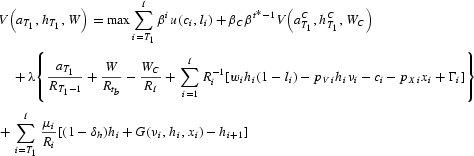
At each date, a unit mass of households is born that lives for I periods. Households are inactive until age T1. They work and accumulate human capital until they retire at age TR. At age t*, each household has one child, who receives its human capital endowment at parental age TH≥t*. Parents leave a bequest (WC) to the child at age I. The household's objective is to maximize discounted lifetime utility:
4 Household variables are generally indexed by date t and age i. To simplify notation, date subscripts are omitted when there is no risk of confusion (e.g., hi instead of ht,i).
subject to
The first term in the objective function (1) reflects the utility obtained from own consumption (c) and leisure (l), while the second term adds the utility of the child, which is valued with a weight of βC. The household's endowments are
units of physical capital,
units of human capital, and an inheritance of W received at age tb=I−t*+1. Equation (2) is a flow budget constraint where the inheritance received is added at age tb, and the bequest left (WC) is subtracted at age I. Income consists of interest (r) earned on physical capital holdings, labor earnings, and lump-sum transfers (Γ). The household spends on consumption goods and on human capital investments. The latter consist of time inputs (νi) and goods inputs (xi), which are purchased at prices pV and pX, respectively. The household receives a wage of w per efficiency unit of time spent in the market, hi (1−li). From age T1 to TR, the household works and engages in job training, which augments human capital according to (3). After age TR the household is retired, which imposes li=1,νi=xi=0.
5 In the interest of comparability with previous research, I treat the ages of labor market entry and exit as fixed. Studying how taxation affects entry and exit decisions is left for future research.
Equation (4) specifies how human capital is transmitted from one generation to the next. Children inherit a weighted average of parental human capital
and of average human capital of the parent's cohort
. Of course, in equilibrium,
. Alternative models of intergenerational human capital transmission have been proposed in the literature, but do not nest IH and pure OLG models as special cases. For example, Becker and Tomes (1986) propose an expression similar to (4) for the transmission of innate skills, which could be thought of as genetic endowments. In addition, parents invest in their children's human capital. Local peer effects lead to intergenerational persistence in Fernandez and Rogerson (1996). In Jovanovic and Nyarko (1995), children learn by observing their parents. Empirically, the various transmission mechanisms are hard to distinguish [Mulligan (1999)]. Perhaps for this reason, no generally accepted theory has emerged.
For the purpose of studying tax policies, the key issue is whether intercohort persistence responds to taxation. This might be the case if parental investment in children is important but not if children learn by observing their parents. Neither IH nor OLG models capture such effects.
The model nests a number of interesting special cases. The model reduces to a pure OLG model if the endowments of new cohorts are fixed exogenously (ω=0) and parents are not altruistic (βC=0). It reduces to an IH model if parents are fully altruistic (βC=1), intercohort persistence is complete (ω=1), human capital is perfectly inherited (ε=1), and parents take this inheritance into account when making investment decisions (ψ=1). The specification chosen here also encompasses intermediate cases in which the intergenerational transmission of human capital is imperfect (ω<1) or only partly internalized (ψ<1).
A parameter of key importance for the subsequent analysis is the elasticity of the human capital endowment with respect to the human capital of the parental cohort (ω). In Section 2.4, I argue that ω is closely related to, but not identical to, measures of intergenerational earnings persistence. For this reason, as well as for lack of a better term, I call ω the degree of intercohort persistence.
Firms
There is one good sold in a competitive market. A single representative firm rents capital (K) and labor (L) from households to solve a standard static profit maximization problem. The technology is F(K,L)=AKθL1−θ, implying competitive rental prices for capital and labor of
where k=K/L. Measured output excludes aggregate job-training expenditures (IX): Y=F(K,L)−IX [Prescott (1998)].
Government
The structure of tax and transfer policies mimics Trostel's (1993) structure. The government levies taxes on capital and labor income to pay for government spending (S) and transfers (Γ). The budget is balanced in each period. The revenue from wage taxes is τL w* L. In addition, the household purchases goods inputs (IX) in the market. A fraction dX of these is tax-deductible, which reduces revenues by an additional τLdXIX. The remainder is subsidized at rate sX, which reduces revenues by an additional (1−dX)sXIX. Capital tax revenues are τK K(r*−δK), which excludes tax-deductible depreciation.
Given these policies, the prices faced by households are w=(1−τL)w* and r=(1−τK)(r*−δK). The price for purchased goods inputs in job training is
Own time in training costs pV=(1−τL)w*. Transfers are paid in equal amounts to all households aged T1 or above. The government budget constraint is therefore
where NtA=I−T1+1 is the size of the adult population.
Parameters
This section describes the choice of baseline parameters, summarized in Table 1. To ensure that my findings are comparable to those in the literature, the choices are largely based on Trostel's (1993) widely cited study. However, since his is an IH model, a number of additional choices need to be made for the OLG versions of the model.
Demographics
As is common in the literature, I assume that agents enter the model at age T1=20. They retire at age TR=64 and die at age I=74. Children are born at parental age t*=28 and receive their human capital endowment in the middle of childhood at age 10 (TH=38).
Preferences
The utility function is of the standard isoelastic form u(c,l)=(clρ)1−σ/(1−σ). The discount factor β is chosen to replicate a capital output ratio of 2.5. The choice of σ=2 is conventional. The value of ρ is chosen to generate a sensible labor-supply elasticity. Most econometric studies find negative labor-supply elasticities for men and slightly positive ones for women [Killingsworth (1983)]. Lucas (1990, p. 306) considers an uncompensated labor-supply elasticity of 0.1 to be an upper bound. I therefore set ρ=0.5, which generates an uncompensated labor-supply elasticity of 0.16. Given that, in U.S. data, most households do not leave bequests to their children, the baseline model features selfish parents and sets βC=0, as in a pure OLG model. I also consider the case where parents value the welfare of their children as much as their own, as in an IH model (βC=1).
Technology
I normalize A=1 by choosing units of output. As in Trostel (1993), the parameter governing the capital share is set to θ=0.25. The depreciation rate is chosen to match an investment share of I/Y=0.17.
Human capital
For the human capital production function, I assume the conventional functional form G=B(vt ht)α xtϕ. B is normalized to 1. The fraction of human capital that is transmitted from parent to child (ε) is chosen to generate wage growth of 60% between the ages of 25 and 48. As in Trostel (1993), the returns to private inputs, α+φ, are set to 0.6. However, I deviate from Trostel's factor shares (α=0.45, φ=0.15) based on Mincer's (1993) estimate that the cost shares of time and goods in job training are similar (α=φ=0.3). The depreciation rate of human capital is δh=0.04 as in Trostel (1993).
Intercohort persistence
Evidence on intergenerational earnings persistence provides the most natural basis for choosing the parameters governing intercohort persistence. Imagine a model identical to the one studied in the paper, except that agents within a cohort are endowed with heterogeneous human capital endowments that are stochastically transmitted from parents to children. If there are no intergenerational spillovers (ψ=1), then human capital is transmitted solely from parents to children according to (4), which becomes
. Hence, a consistent estimate of ω could be obtained by regressing log earnings of parents at the age of human capital transmission on log earnings of the children early during their work lives.
This is very similar to a common measure of intergenerational earnings persistence, which is the coefficient ω1 in a regression of the form
Here, the unit of observation is a parent–child pair, yP and yC are measures of parental and child earnings, and ζ is a random-error term. Even though these regressions are meant to capture lifetime earnings persistence, data limitations force researchers to proxy for lifetime earnings using short averages of parental and child earnings at ages that are roughly consistent with the ages of human capital transmission in my model. Since estimates of intergenerational earnings persistence are on the order of 0.5, I set the baseline value of ω to 0.5.
6 Most estimates cited in Mulligan's (1997) survey of intergenerational earnings persistence lie between 0.2 and 0.6. Attempts to correct for measurement error and nonrepresentative samples result in estimates at the high end of this range.
The main limitation of this approach is that human capital may be partly transmitted through intergenerational spillovers (ψ<1). In that case, intergenerational earnings persistence is a downward-biased estimator of ω. The intuition is as follows. If parental human capital
rises by x, then the human capital average that determines the child's endowment in (4) rises by less than xω. Therefore, regressing child earnings on parental earnings yields an estimate of ω1, which is less than ω.7
To prove that the bias is negative, rewrite the error term in (7) as
, where ζ0 is a constant, and note that ζi is negatively correlated with the regressor.
What matters for tax effects is therefore not intergenerational mobility, but the degree to which human capital is transmitted from one cohort to the next. While it would be desirable to find a method of estimating ω in the presence of such spillovers, this is beyond the scope of the paper. The analysis therefore maintains ω=0.5 as a benchmark value, but explores other values in the sensitivity analysis. Note that the value of ε goes not affect intercohort persistence. Instead, ε and
B jointly determine earnings growth over the household's life cycle. One of the parameters (
B) may be normalized to unity by a choice of units. The other (ε) is chosen to match 60% wage growth between the ages of 20 and 48 [Duncan and Hoffman (
1979)].
Policy parameters follow Trostel (1993) in setting τL=τK=0.4 and S/Y=0.15. One quarter of goods inputs in job training are purchased with foregone earnings (dX=0.25); the remainder is subsidized at a rate of sX=0.6. Transfers balance the budget.
NUMERICAL EXPERIMENTS
This section examines how the steady-state and transitional effects of tax changes depend on intercohort persistence. The policy experiments consist of permanent, unanticipated cuts in tax rates by 10% (from 0.4 to 0.36) financed by reductions in lump-sum transfers. For each experiment, I report the steady-state tax elasticities of human capital, physical capital, and output (H,K,Y).8
The tax elasticities are defined as E(X)=(dX/X)/(dτ/τ), where τ is the tax rate changed in the experiment.
I also report half-lives of
Y for the transition between steady-states, defined as the time period after which output remains within half the date-1 distance from its new steady-state value.
Finally, I calculate the changes in welfare levels, defined as the proportional change in consumption required to make each cohort indifferent between the initial steady-state and the path following the tax change. More precisely, if the age profiles of consumption and leisure are
in the initial steady-state and (ci,li) in the steady-state under the new tax rate, then the welfare gain (Ω) is defined by
Each tax experiment is performed for a sequence of models, so as to decompose the differences between a pure OLG model and an IH model into the contributions of individual model features. Table 2 summarizes the assumptions underlying each model. Model M1 is a pure OLG model with finite horizons and no intergenerational links (ω=0; βC=0). Model M2 is the benchmark case. It adds incomplete persistence of human capital to M1, where ω is set to 0.5 based on estimates of intergenerational earnings persistence. Persistence is complete in model M3 (ω=1). Model M4 adds persistence of physical capital via altruistic bequests (βC=1), but parents do not internalize the intergenerational transfer of human capital (ψ=0), whereas they do in model M5 (ψ=1). Model M6, finally, is an IH model.
Note that each model differs from the previous one only by a single feature. The exception is the IH model M6, which changes a number of demographic features at a time (t*=TH=I+1, TR=I, ε=1). This setup permits us to precisely identify the significance of each feature that distinguishes the IH from the pure OLG model. The fact that the properties of the IH model are very similar to those of model M4 verifies that it is indeed intergenerational links that drive the larger tax elasticities in the IH case and not any of the other features that differ implicitly between IH and OLG models.
Steady-State Results
This section discusses the comparative steady-state effects of tax reforms; transitional dynamics results are presented below. Tables 3 to 5 report the findings for reductions in wage, capital, and income tax rates by 10%, respectively. The main findings can be summarized as follows:
- Intercohort persistence strongly affects the response of human capital to tax changes. The steady-state tax elasticities of H more than double for all tax experiments as persistence rises from none in M1 to complete in M3. Stronger persistence is generally associated with larger tax elasticities of H.
- The two models familiar from the literature generate very different tax elasticities. In the IH model (M6), the changes in human capital, physical capital, and output are more than two times larger than in the pure OLG model (M1). This holds for all tax experiments.
- In the wage tax experiment, the difference between the IH and the pure OLG model is almost entirely due to intercohort persistence of human capital. Comparing the outcomes of M4 and M6 shows that other differences between IH and OLG models, including parental altruism, play only a minor role.
- In the capital tax experiment, the outcomes depend mostly on the presence of a bequest motive.
- Even with complete persistence of human capital, tax elasticities differ between OLG (M3) and IH models (M6). This discrepancy is almost entirely due to the bequest motive implicit in the IH model. Once a bequest motive is added to the OLG model with complete persistence (M4), its properties are similar to those of the IH model.
- If the intergenerational transmission of human capital is internalized by the parent, the tax effects tend to be larger than in the case of an intergenerational human capital spillover (M5 vs. M4).
- Intercohort persistence strongly affects the steady-state welfare changes. In the wage and income tax experiments, increasing persistence from none to complete raises the welfare gains more than sevenfold.
Discussion
Taken together, these findings show that the intercohort persistence of both physical and human capital has an important impact on the predicted tax effects. Next, I discuss the economic intuition underlying these results.9
Additional intuition for the signs of the tax effects and for their dependence on parameters can be found in Trostel (1993) or in Engen et al. (1997).
Consider first the effect of taxing labor income in the pure OLG model, M1. The lower after-tax wage rate reduces labor-supply and human capital investment. As a result, H and L decline. The interest rate falls, which reduces saving and the capital stock, K.
Intercohort persistence in model M2 magnifies the human capital response. To gain intuition for this result, it is useful to imagine a sequence of cohorts, the first of which is born at the date of the tax change. Without intercohort persistence, the human capital endowments,
, of all cohorts are given, but their adult human capital,
, is reduced. By contrast, with intercohort persistence, the endowment is unaffected only for the first cohort. The second cohort starts with a smaller endowment because its parents invested less in human capital. The endowment of each subsequent generation is reduced somewhat more that that of its predecessor. Stronger intercohort persistence amplifies this feedback mechanism.10
An analytical characterization of the relationship between intercohort persistence and tax effects is provided by Hendricks (2000).
This argument suggests that the role of intercohort persistence should increase over time. This intuition is born out by the transitional dynamics results discussed below.
The main effect of altruistic bequests is to fix the after-tax interest rate. For the wage tax experiment, this does not have a strong effect (compare M4 with M3), but it plays a large role for the capital tax experiments discussed below. Internalized persistence leads to a larger drop in human capital because the value of the human capital passed on to the children declines because of the wage tax.
Consider next the effect of taxing capital income, shown in Table 4. In the pure OLG model (M1) the lower interest rate reduces investment and the capital stock, K. This, in turn, lowers the wage rate and thus labor-supply and H. On the other hand, the lower interest rate raises the present-value of earnings generated by an additional unit of human capital. The net response of H is therefore ambiguous. For model M1, the two effects roughly balance each other and H remains nearly unchanged.
For the reason explained earlier, intercohort persistence magnifies the response of H. As a result, the tax elasticity of H is larger for models M2 and M3, and K declines less compared with M1. Most of the difference between the pure OLG model and the IH model is due to parental altruism. In the models with bequests, the after-tax interest rate is fixed. Higher capital taxes then reduce the steady-state K/H ratio. This depresses wages and human capital investment. By contrast, in the absence of a bequest motive, the after-tax interest rate drops so that the stock of human capital actually rises in response to higher taxes.
Internalized persistence magnifies the response of H for the same reason as in the wage tax case. The income tax experiment combines the effects of wage tax and capital income tax changes.
Varying the degree of persistence
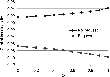
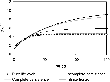
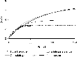
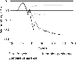
To further clarify the relationship between persistence and tax effects, Figure 1 shows steady-state wage tax elasticities of human capital for the entire range of persistence levels (ω=0 to ω=1). Higher persistence is associated with larger (absolute) tax elasticities, even if the model allows for altruistic bequests. Since the relationship is slightly concave, the errors introduced by understating persistence are smaller than those introduced by overstating persistence. The impact of persistence is similar for capital taxes (see Figure 2), even though the signs of the elasticities change when the bequest motive is introduced.
Wage tax elasticities of human capital.
Capital tax elasticities of human capital.
An important question is under which circumstances the models studied in the literature approximate an environment with realistic intercohort persistence. Given the benchmark value of ω=0.5, neither the IH model nor the pure OLG model approximates the outcomes of realistic persistence very well. The benchmark model implies a wage tax elasticity of human capital near −0.4, compared with −0.3 for the pure OLG model and −0.7 for the IH model. Bequests slightly reduce the importance of intercohort persistence (see Figure 1). For the capital tax experiment, pure OLG and IH models differ from realistic persistence by roughly equal amounts.
Of course, given the uncertainty about the value of ω, these calculations should not be viewed as conclusive. In particular, if intergenerational human capital spillovers are strong, then ω should be larger than 0.5 and the IH model could be close to a model with realistic persistence. Finding ways of measuring ω and ψ is an important task for future research.
Sensitivity analysis
To further investigate the robustness of the finding that persistence is an important determinant of tax elasticities, Table 6 considers variations of the baseline parameter values. Steady-state wage and capital tax elasticities of human capital are shown for three model versions: pure OLG (M1), incomplete persistence (ω=0.5, M2), and complete persistence (M3). The last two columns show by how much the higher persistence of models M2 and M3 increases tax elasticities. Each row changes only one parameter compared with the baseline case.
The first part of the table explores parameter changes that can be shown analytically to affect the importance persistence [see Hendricks (2000)]. These include higher returns to scale in the production of human capital (α=φ=0.35), a lower share of goods inputs (α=0.45, φ=0.15) as in Trostel (1993), and variations in the rate of human capital depreciation (δh=0.01 or δh=0.1). Finally, Hendricks (2000) shows that tax elasticities rise with age. Therefore, the age at which children inherit their human capital should matter. The table shows the case in which children are born late in their parents' life (TH=54). The second part of the table examines parameters that are known to be important for the magnitude of tax elasticities in IH models. These include preference parameters governing the intertemporal elasticity of substitution (σ) and the labor-supply elasticity (ρ).
The general conclusion from the sensitivity analysis is that persistence remains important in all cases. The model with incomplete persistence yields wage tax elasticities between 22% and 59% greater than the pure life cycle model. The tax elasticities in the complete persistence case are still larger by 29% to 154%. The only parameter change that substantially reduces the role of persistence compared with the baseline case is the higher depreciation rate of human capital. However, the value δh=0.1 is almost surely larger than reasonable in an OLG model.11
Depreciation rates of human capital should be larger in IH models where the rate encompasses depreciation over the life cycle as well as depreciation at death. Nonetheless, Stokey and Rebelo (1995) argue that even in IH models a depreciation rate of 0.1 is most likely too high.
The findings for capital taxes are similar (see
Table 7).
Transitional Dynamics Results
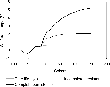
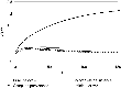
This section discusses how intercohort persistence affects the transitional dynamics following unannounced tax changes. For a cut in the wage tax from 0.4 to 0.36, the time paths for output and aggregate human capital are shown in Figure 3. Three versions of the OLG model (M1, ω=0; M2, ω=0.5; and M3, ω=1) are compared with the IH model (M6).12
For OLG models with bequest, motive transition paths are not computed because they do not converge to steady-states after a permanent tax change. The reason is that consumption does not regress to the mean within a dynasty.
Qualitatively, the trajectories implied by all models are similar and exhibit the monotone convergence patterns well known from pure OLG and IH models. The higher after-tax wage rate causes households to invest more in training. As the human capital stock is built up, the wage rate declines, so that training eventually levels off and the economy approaches the steady-state.
Time paths of output following a reduction in wage taxes.
Time paths of aggregate human capital following a reduction in wage taxes.
The main new finding is that higher persistence substantially reduces the speed of convergence to the steady-state. The half-life of output rises from 13 years to 40~years as persistence increases from none to complete. These figures are consistent with the rates of convergence reported in the literature for pure OLG and for IH models [e.g., Davies and Whalley (1991), Trostel (1993)]. Decomposing the differences between the two models into the contributions of various assumptions reveals that intercohort persistence of human capital is mainly responsible for the slower convergence found in IH models. With complete persistence, the OLG model generates time paths that are very similar to the IH model.
Convergence is relatively rapid in the pure life cycle model because the endowments of physical and human capital received by new generations are fixed. Cohorts born after the date of the tax change start out with endowments that are consistent with the new steady-state. Their behavior differs from the steady-state only because prices temporarily deviate from steady-state levels.13
Davies and Whalley (1991) discuss the rate of convergence in a pure OLG model.
By contrast, if human capital is transmitted across generations, the endowments of new cohorts are initially below their steady-state level and building them up to steady-state levels takes several generations. Note that all time paths are very similar for the first 20 years because it takes this long until the first cohorts born after the tax change enter the model.
Figure 4 shows how the wage tax reduction affects the welfare of different birth cohorts in the OLG models (M1 through M3) in. Qualitatively, the findings match those of pure OLG models [see Auerbach and Kotlikoff (1987)]. Reducing the wage tax hurts the initial old because they no longer receive earnings, while their lump-sum transfers are cut in order to balance the government budget. Younger cohorts, by contrast, benefit from the lower tax distortion. Welfare gains rise over time and are larger for higher persistence. The reason is that the human capital endowments of new cohorts rise more strongly when persistence is higher.
Welfare effects of a wage tax reduction.
Transition paths following a reduction of the capital income tax rate from 0.4 to 0.36 are shown in Figure 5. In the pure OLG model, output rises and human capital declines almost monotonically after the tax change. As explained earlier, the output response is driven by increased investment in K, whereas the human capital response is the net effect of two offsetting forces: A higher wage rate induces more human capital investment, while wealth effects reduce hours worked and hence the return to training. For the model parameters, the latter force slightly outweighs the former, and human capital declines.
Time paths of aggregate output following a reduction in capital taxes.
Time paths of aggregate human capital following a reduction in capital taxes.
As in the wage tax case, transitions are more drawn out when persistence is higher. The intuition is similar: The human capital endowments of new cohorts fall over time because previous cohorts invested less in training.
A striking observation is the large discrepancy between the OLG models and the IH model. The capital response to the tax change is much larger in the IH model due to the infinite interest elasticity of saving. The higher capital stock increases the wage rate and induces additional human capital investment. As a result, H eventually increases above its initial level. The initial dip in H is the result of asset substitution. Additional investment in K is partly financed via lower investment in H. This is profitable because the wage rate does not increase until K has been accumulated.
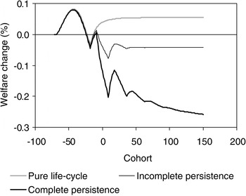
The welfare changes due to a capital tax cut are shown in Figure 6. In the pure OLG model, the initial old cohorts benefit because their capital return increases. The initial young, who were born before the tax change, are hurt by lower wages; they overinvested in the past. The young born later on benefit from the reduced distortion [see Auerbach and Kotlikoff (1987) for more discussion]. Intercohort persistence does not change the general pattern of welfare changes, but the magnitudes are larger, especially for the later cohorts. The reason is that the human capital endowments of later cohorts change by larger amounts.14
The sawtooth pattern of the welfare changes in models with intercohort persistence reflects the fact that a cohort's welfare depends on the exact cohort of the parents via the human capital endowments. These unusual dynamics are an artifact of two model features: All agents within a cohort are identical and human capital is transmitted from parent to child not over a period of years but at a point in time.
Note that neither the model with complete intercohort persistence nor the pure OLG model very closely approximates the welfare changes of the benchmark model with realistic persistence.
Welfare effects of a capital tax reduction.
CONCLUSION
The question of how taxes affect human capital accumulation has been studied extensively in the context of two classes of models: overlapping generations and infinite horizon. These two model classes embody very different assumptions about the intergenerational transmission of human and physical capital. In pure OLG models, the endowments of new agents are exogenous and there is no intercohort persistence. By contrast, persistence is implicitly complete in IH models. The question addressed here is how these differences in persistence affect the responsiveness of human capital to wage and capital income taxation.
The main finding is that stronger persistence implies larger steady-state tax elasticities and slower rates of convergence to the steady-state. An important implication is that the two model classes studied previously generate very different predictions about long-run tax effects. IH models generate larger tax elasticities than OLG models with incomplete persistence, even if cohorts are altruistically linked. For the tax experiments studied here, these differences are large. Models with complete persistence yield tax elasticities at least two times larger and half-lives at least three times larger than do models without persistence. These findings contrast sharply with the common view that IH models and OLG models “have very different theoretical structures, yet in practice, for the kind of tax problem under study here, seem to yield quite similar results” [Lucas (1990, p. 295)]. While it is true that OLG models with complete persistence of human and physical capital yield results very similar to IH models, the two model classes generally do not have similar properties.
An important task for future research is therefore to measure intercohort persistence in the data. One promising approach relates the model's persistence parameters (ω, ψ) to measures of intergenerational mobility commonly estimated in the literature [e.g., Mulligan (1997)]. Plausible values for intercohort persistence are then near 0.5, in which case neither pure OLG models nor IH models offer good approximations for a model with realistic persistence. This holds true for the steady-state and transitional effects of all the tax experiments studied in this paper.
The findings presented in this may have important implications beyond the study of tax policies. For example, a recent branch of the growth literature studies whether human-capital-augmented growth models can account for two important development facts: for the large cross-country income differences observed in postwar data and for the observed speed of convergence to steady-state.15
See Mankiw et al. (1992), Prescott (1998).
This question has been studied in the context of IH models in which tax distortions cause some countries to underinvest in human and physical capital. The findings here suggest that the extent to which the standard growth model can account for both observations should depend on intercohort persistence.
APPENDIX A: DEFINITION OF EQUILIBRIUM
HOUSEHOLD OPTIMIZATION
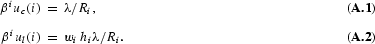
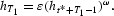
The Lagrangean for the household problem can be written as
where
is a cumulative discount factor. It is assumed that the solution is always interior and satisfies
, except during retirement. The first-order conditions are
For the job-training period (i=T1,…,TR−1),
During retirement,
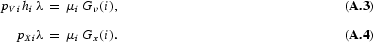
. The first-order condition for hi is
If the intergenerational spillover is internalized, the marginal value of augmenting child human capital must be added to (A.5) at age
. The derivative of the value function is
Finally, bequests are determined by
where
. This can be simplified to
EQUILIBRIUM CONDITIONS
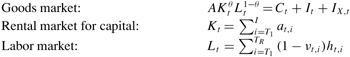
Define the following aggregates:
The market-clearing conditions are then
An equilibrium is a sequence of prices
, aggregate quantities
, an endogenous policy variable, and household age profiles
and bequests
that satisfy
- at,1=0 and obeys the conditions for intergenerational links;
- firms maximize profits;
- prices are determined as described in the government section;
- the government budget constraint is met at each date;
- Households maximize utility, given paths of prices, so that the age profiles obey (A.1) through (A.6), the laws of motion, and the present-value budget constraint;
- markets clear.
STEADY-STATE CONDITIONS
If the economy is in steady-state, the equilibrium conditions simplify as follows. Dropping generation subscripts, denote by hi the age profile of the household born at date 1. The bequest condition (A.7) becomes
. This implies a condition familiar from IH models:
. The aggregate bequest flow per period is
. Since parents are t*−1 years older than their children, the intergenerational spillover condition becomes
Aggregate investment in job training is
. Analogous conditions hold for aggregate consumption, and the supplies of capital. Investment in physical capital obeys I=δKK. The market-clearing conditions remain unchanged.
APPENDIX B: THE INFINITE HORIZON CASE
The firm's problem and the government budget constraint are the same as in the baseline model. They yield three equilibrium conditions: the government budget constraint and the cost-minimizing factor prices.
HOUSEHOLDS
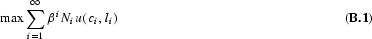
A standard infinite horizon (IH) model emerges as a special case of the baseline model, if the following assumptions are maintained:
- Children are born after the parent has died (t*=I+1).
- Households do not retire (TR=I).
- Generations are linked by an altruistic bequest motive with βC=1.
- Parents can bequeath not only physical but also human capital (ω=1, ψ=1, ε=1), so that h1C=hI+1.
Under these conditions, the parent's problem simplifies to
where
is a cumulative discount factor. Since the child inherits all human capital, the laws of motion for h and a collapse to their IH versions. Similarly, since
, the parent's utility function collapses to the IH version
.
Since the child is born after the parent dies (at parental age I+1), it receives the bequest at the beginning of its first period. Equivalently, it receives the bequest plus interest in the first period. Therefore, the first-order condition for the bequest left is
Instead of μI=0, we have
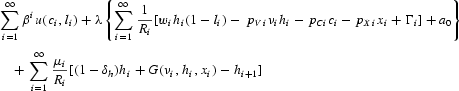
. Households then solve the problem
subject to a1, h1, given
This specification slightly generalizes the one derived as a reduced form of the life cycle model with bequests in that it allows for population growth. It is assumed that the solution is always interior and satisfies
. It is further assumed that a present-value budget constraint holds:
where
and R0=1. Write the Lagrangean as
The first-order conditions are
Define
. Then (B.7) through (B.9) can be rewritten as
For computational purposes, it is useful to reduce the dimensionality of the problem. Taking ratios of (B.5) and (B.6) yields
Similarly, the ratio of (B.7) and (B.8) is
Substituting (B.8) into (B.10) allows us to eliminate η:
EQUILIBRIUM
Define the following aggregates:
. Given initial conditions (a1, h1), an equilibrium is a sequence of prices (r,w,r*, w*, pX, pV, pC) and quantities (K, L, a, h, ν, x, c) plus one endogenous policy variable that satisfy
- 1the firm's first-order conditions;
- the definitions of the prices, given policy variables;
- the household's first-order conditions shown above together with the present-value budget constraint and the laws of motion for h and a shown in the household problem;
- the aggregation conditions;
- the government budget constraint;
- the market-clearing condition (which is redundant), F(K, L)= C+I+X+S.
STEADY-STATE
In steady-state, quantities, prices, and shadow prices (λ, μ) are constant. Ri= (1+r)i. The endogenous variables (a, h, x, ν, c, l, μ, λ) are determined by the household first-order conditions (B.5) through (B.9), the laws of motion for a and h, where it is imposed that both grow at rate γ, and the present-value budget constraint (B.4). In addition, one policy variable is determined endogenously to satisfy the government budget constraint. The law of motion for h becomes 1=(1−δh)+Gh. The first-order condition for c implies the usual Euler equation: β=1+r.
For helpful suggestions, I am grateful to Lee Ohanian. I also wish to thank two anonymous referees and an associate editor for their comments.