PREAMBLE
I started working on this paper when I was working in the MEDS Department at Northwestern University, an extremely stimulating place for a theorist. I had been puzzled by use of lotteries in General Equilibrium models, which I first encountered in the paper on contracting by Prescott and Townsend (1984). That paper made me think, hard, about the social value of randomization—when would it be valuable, why was it valuable in the Prescott and Townsend setting, and so on. Was this something that would always work when there was a nonconvexity in the individual's feasible set?
At some point, I realized that if I was going to understand the problem better, I would need to think about it in a much simpler setting than where they were working. This led me to consider a simple setting in which there were two goods, one divisible and one indivisible. It was in thinking about that simple version of the problem that I realized that in a setting such as that, the indirect utility of wealth would have a nonconcave region, much like that envisioned by Friedman and Savage in their paper on choice and risk (1948). It was not exactly the same, however, as this nonconcave region was bounded above and below by regions of strict concavity. This difference is important for understanding who would gamble—the middle income and the rich in the Friedman and Savage approach and the middle income group here.
The note also included two other examples beyond that first basic one. Both were designed to show that there were interesting and realistic cases when there were indivisibilities in goods but not a nonconcavity in the indirect utility of wealth. One of these was based on quality differentiation with increasing marginal cost of quality and the second was a simple continuous time example showing that division over time could act as a substitute for randomization.
Soon after writing the note, it was pointed out to me (by Mark Machina) that the first example was already known. Indeed, it had appeared in 1965 in a short paper by Kwang (1965). Because that example was the one that I found most interesting and it had already been done, I set the project aside and went on to work on other things.
Since then, the Rogerson (1988) approach to labor supply as an indivisible good and the use of lotteries to decentralize efficient allocations has become more and more popular.1
I have not made an attempt to include a complete set of references of papers that use that approach here. See Hansen (1985) and Prescott and Rios-Rull (1992) for examples.
To put this topic into a larger context, note that there is an important debate going on in the literature now (and over the years since this note was first written). It concerns the responsiveness of labor supply to changes in policy both at the level of the individual and the aggregate. The answers to these questions typically depend on one (or two) key parameter(s)—the elasticity of labor supply, or, at a deeper level, the parameters of preferences determining this elasticity, for example, the intertemporal elasticity of substitution of leisure.
Although this debate is diverse, it is useful to frame it as a discussion between two camps. The traditional labor economists say that they know the answer to these questions based on micro studies of labor supply. This is that labor supply is very inelastic. The other camp argues that it is quite elastic.
The Rogerson approach, as it is typically implemented, has the implication that labor supply is quite elastic—once lotteries are introduced, the utility function is effectively linear in leisure. This is standard in Expected Utility models, utility is linear in probabilities. In the Rogerson approach, it is these probabilities that map directly into the analog of labor supplies. This, along with other features, has been used as an argument against the model by micro labor economists.
In the continuous time version of the model with indivisibilities, the linearity of utility in leisure comes from a slightly different source. It is directly from the indivisibility of working instant by instant—either you are working at t, or you are not. Because of this, in certain cases, the effective margin for determining labor supply is something like the “fraction of time spent working.” This analogy is exact in some, but not all, cases (separable utility and balanced growth behavior of prices are sufficient in the example). And it is because of this property that lotteries are irrelevant (i.e., have no social value) in examples like this.
The second is a more palatable interpretation for most people, but the two models give rise to the same aggregate implications [see Ljungqvist and Sargent (forthcoming)].
Because of this debate and its importance, I have changed only one substantive thing in the note this time around. This is to add a set of sufficient conditions under which the indirect utility function over wealth is concave in the continuous time setting even with discounting. When these conditions are met, and a balanced growth interest condition also holds, the continuous time model is concave, and looks very much like a model with lotteries already included. Here, the relevant margin for labor supply is the fraction of time spent working, and utility is linear in this quantity. Because of this, labor supply will be, as in Rogerson, very elastic.
INTRODUCTION
In their 1948 paper on decisions under uncertainty, Friedman and Savage presented a puzzle. This is the empirical fact that many individuals both gamble and buy insurance. The puzzle in this observation is that the fact of gambling seems to imply risk-loving, whereas that of insurance purchase implies risk-aversion. The difficulty is then the reconciliation of these two seemingly contradictory behaviors. Friedman and Savage proposed a solution to the puzzle which involved a utility function which is first concave and then convex. This formulation allows for the possibility of both risk-taking and insurance by the same individual.
The purpose of this note is to propose a slightly different solution to this puzzle. In the model presented here, agents are expected utility maximizers with preferences that are strictly concave and yet, optimal choices by individuals involve both gambling and the purchase of insurance. At this point, the natural question to ask is: What is the trick? (Of course, there must be one.) The answer lies in our choice of consumption set. In the simplest version of the model, the consumption set consists of R×{0, 1}. We will interpret the first coordinate of this, (m, h), as money, the second as some indivisible good such as a house, a trip, or some other expensive but indivisible good. It is this indivisibility (quite reasonable in practice) that is the driving force in the examples.
Of course, with the presence of an indivisibility in the consumption set, concavity of the utility function is not defined in a strict sense. What we will mean by this is that the expected utility function is the restriction to the consumption set of a function strictly concave on R2.
Although the motivation here is quite different, it is easy to see that this formulation of the problem induces an indirect utility function over money (the price of the indivisible good is known with certainty ahead of time), which features a nonconcavity of the Friedman and Savage type. There are important differences, however. In particular, although the Friedman and Savage assumptions would lead one to expect that the rich would gamble and the poor would buy insurance (assuming the same tastes), our approach would lead to the opposite conclusion. In essence, within the model, individuals gamble in order to acquire the ability to “jump across” the indivisibility in the consumption set. This is neither necessary nor desirable for an agent with high initial wealth.
The reader will note the strong similarity between this model and recent results concerning the possibility of the benefits (social) from lotteries arising in competitive systems. Notable contributions to this literature include Prescott and Townsend (1984), Rogerson (1988), and Prescott and Rio-Rull (1992).
Although the results noted here are interesting, it is rare in practice that a good is indivisible to the extent utilized in the example. There are often possibilities for effectively convexifying the consumption set through the availability of continuous gradation of quality or characteristics [e.g., the Rosen (1974) and Mas-Collel (1975) models] or timing. Some initial investigation of these mitigating possibilities is offered in Section 5.
AN EXAMPLE
Consider an agent who at time 2 must choose how to split his income, m, between consumption of money and an indivisible good. Let x1 denote his consumption of money and x2 his consumption of the indivisible good. We will constrain x2 to be 0 or 1. Assume that his utility is given by

.
Thus, preferences are separable in the two goods. Suppose that the agent's initial endowment is random, on money only with p(m=0)=p(m=2)=1/2 and that the cost of the indivisible good is p=3/4.
Finally, assume that the uncertainty in his income is resolved at time 1. It is straightforward to check that if m=0 the agent's final consumption is (0, 0) and that if m=2, his consumption is given by (5/4, 1). Assuming that u represents his preferences over risk as well, we see that his expected utility at the initial endowment is given by

Would this agent buy “fair” insurance? As it turns out, the answer is yes. This gives him m=1 with probability one. With m=1, the agent is indifferent between buying the second good and not. Thus, his expected utility with fair insurance is

The story does not end here, however. Consider a lottery ticket that costs 7/16 and pays off 0 with probability 5/12 and 12/16 with probability 7/12. (Note that this lottery ticket is fair in that its expected payout equals the ticket price.) If the agent purchases both the insurance and the lottery ticket his distribution over final wealth is given by m=9/16 with probability 5/12 and 21/16 with probability 7/12. It is optimal in this case for him to set x2=1 if he wins and x2=0 if he loses.
This gives him expected utility of

Of course, u2 > u1 > u0. Thus, the agent will buy both the insurance policy and the lottery ticket. As it turns out, buying complete insurance and the lottery ticket as specified is in fact the best the agent can do in terms of fair gambles and insurance. (This is shown in the next section.) Finally, after the lottery, the agent will not gamble again. That is, the gambling that the agent does must put the right mass in the right locations, and because of this (and the Strong Law of Large Numbers), this theory would be unable to rationalize repeated gambling with a negative expected value. This is also shown in the next section.
THE BASIC MODEL
Consider an individual agent facing a decision problem under uncertainty. Let X = R+×{0, 1}. This is assumed to be his consumption set. As noted in the Introduction, we will interpret a point (x1, x2) ∈ X′ as consisting of money or some appropriate aggregate Hicksian commodity and the consumption of some indivisible choice such as housing, career choice or residential location.
Assume that the individual has preferences, [scsim ], over probability distributions μ on X which we will denote by Δ. We will assume that the preferences satisfy the relevant version of the von neumann-Morgenstern axioms [see, e.g., Grandmont (1972)] so that preferences can be represented by an expected utility function. That is, we will assume that there is a u:X→R such that μ1[scsim ]μ2[hArr ]∫u(x) dμ1≥∫u(x) dμ2 for all μ1 and μ2 in Δ.
Because our aim is only to show that certain things can happen we will make the (strong) assumption that u(x1, x2) = v(x1) + w(x2). This is equivalent to assuming u(x1, 0) = v(x1) and u(x1, 1) = v(x1) + δ. We will assume that u is strictly increasing, strictly concave and C1 and that δ > 0.
For simplicity, we will assume the agent starts with a random endowment only on money. Implicitly, we have assumed state independence of the utility function and hence will regard his initial endowment as a probability distribution, μ0 ∈ Δ. Our assumptions imply that μ0(R+×{1}) = 0.
Consider a two-period model. In the first period, the agent buys insurance and/or gambles and the realization of his uncertain income is drawn. There is no consumption during the first period. In the second period, the agent decides on how to split his income between consumption of money and the indivisible good x2. We will assume that at time 1 it is known with certainty that the price of the second good will be p.
We will assume that in the first period the agent faces a (large) risk-neutral market willing to sell him any mean zero random variable. (The risk-neutrality is for convenience only.)
Formally, the agent must choose a “rule” r:R+→X and a probability distribution μ∈Δ subject to

(Note: This formulation of the problem is somewhat clumsy from the formal point of view. Ideally, one would want to choose a state space Ω first, assume that agents are endowed with random income on (ω) during period 1, have agents choose random variables x1(ω), x2(ω) ∈ X subject to the constraint that ∫[x1(ω)+x2(ω)p] dP(ω)≤∫m(ω) dP(ω) [we have imposed the assumption of risk neutrality of a large market by having the price of money identically equal to one—the assumption that p is constant could be justified that p is the value to the market of one unit of the second good]. The difficulty with this approach is in setting Ω in the first place. That is, in a model in which lotteries are “created,” Ω is naturally endogenous to the model. Because there seem to be no natural limits on randomizing devices used to create Ω, this formulation was chosen. If a sufficiently rich Ω was available, the alternative approach could be chosen making the obvious changes along the way. Perhaps this is possible.)
It is easy to see that there is a “best” r for this problem which is independent of μ(a.s.). Let m* be the unique (because of our separability assumption) solution to v(m*−p)+δ=v(m*). It follows that the optimal consumption choice is to set r1(m*) = m, r2(m) = 0 if m ≤ m* and r1(m) = m−p, r2(m) = 1 if m ≥ m*. (Note that at m*, the agent is indifferent between setting r2 = 0 or 1.) In general (i.e., without separability) there may be multiple “switches” between r2 = 0 and r2=1.
Because of this fact, it follows that solving (1) is equivalent to solving
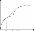
where V*(m) = v(m) if m ≤ m* and V*(m) = v(m−p) + δ if m ≥ m*. (Formally, μ*, r* is a solution to (1) if and only if μ* is a solution to (2) and r* is as described here a.s. μ*.) See Figure 1.

The indirect utility function for wealth.
Note that (2) is simply a (infinite dimensional) linear programming problem. In general, (2) will not have a solution (e.g., if V* was convex) but it is easy to set conditions on v so that a solution exists. One set of conditions is given by
- i. Assume that v(p)−v(0) > δ (this is not essential but simplifies the argument),
- ii. that v′(0)>δ/p and,
- iii. that limm→∞v′(m)<δ/p.
In this case, it follows that m* > p and that there is a unique
for which
. It follows that
. Consider the linear function of m defined by
.
It can be shown that g(m) ≥ V*(m) for all m with equality at
and
. (Although this may look mysterious, the function defined by h(m) = v*(m) if
or
and g(m) otherwise is the concave upper envelope of V*—thus, it is a natural construct to consider.)
Our goal is to completely characterize the solution to (2). There are three cases to consider.
[Case 1:] If
, μ* puts probability one on m0.
- To see this, let t(m) be the tangent line to m0. It follows that t(m)≥V*(m) with equality only at m0. The usual Jensen's inequality argument now can be used. It follows that μ* is unique.
[Case 2:] If
, μ* puts probability one on m0.
- The argument here is the same as in Case 1.
[Case 3:] If
, write
, where 0≤α≤1. Then μ* puts probability α on
and probability (1−α) on
.
As in the standard Jensen's inequality argument, it follows that [since g(m)≥v*(m) for all m]

and the inequality is strict unless
. Note that setting μ* as claimed here gives
, completing the argument.
Summarizing, we have to this point the following:
PROPOSITION 1
For all values of m0, (2) has a unique solution.
If m0 is either sufficiently low
or sufficiently high
the solution to (2) consists of complete insurance. If
the solution to (2) is a lottery on
and
.
Notes
- If μ0 is not degenerate at m0, we can think of the solution, μ*, as arising by the purchase of both insurance and a lottery ticket. For example, if but , the solution to (2) completely insures the agent against outcomes below .
- Clearly the assumption of a risk-neutral market is not necessary here. The fundamental fact that V* is not concave is what is important. The existence of a risk-neutral market just shows this most strikingly (we would not get such a strong conclusion concerning the optimality of gambling if the market was risk-averse).
- The proposition shows that in this simple model at least, we would not expect to see the rich gambling (holding preferences constant).
- The fact that the optimal lottery has only two prizes is not an accident here. As noted earlier, (2) is a linear programming problem. There are two constraints to this problem, so we should “expect” no more than two active variables in the basis.
- The arguments of the proposition are quite general. In particular, as noted in 4, even for more general V*'s, the solution (if one exists) should involve only two m's.
- Note that in the case that , the lottery constructed exhausts all desire to gamble on the agent's part. (This seems to be a type of arbitrage condition.) In particular, after the first period, he has either or . In either case, he would accept no further lotteries. This implies that an effect described by Friedman and Savage will be an outcome. That is, holding preferences fixed, at period 2 there are two “social classes”—those with wealth above and those with wealth below : equivalently, those who buy houses and those who do not.
EXTENSIONS
In this section, we will expand the model of the previous section in two directions. The first is in the direction of multiple qualities, the second concerns the addition of multiple time periods. In both cases, we will show that the results of the previous two section on the existence (and optimality) of lotteries in equilibrium can be overturned in some cases.
Multiple Qualities
Alter the problem considered in Section 4 by allowing the agent to choose from a continuum of qualities. Formally, model the agent's choice at time 2 as choosing an (x1, x2) ∈ R × Q = X, where Q⊂R+ is the set of possible varieties. We will assume that 0 ∈ Q and interpret the choice of a point (x1, 0) as choosing not to buy the second good. (That is, buying a good of quality 0 is the same as not buying one at all.) Note that this is the model of commodity differentiation analyzed by Rosen (1974). This assumes that the agent buys one and only one unit of the second good and that this is of only one quality. [The model of Mas-Colell (1975) is a generalization of this in which the purchase of more than one unit is allowed. This model is formally a special case of that of Mas-Colell's if there are no qualities near zero other than zero itself.]
Assume that at time 2 the agent faces a price schedule p(q) for buying the second good and that this schedule is known (for simplicity) at time 1. Assume that p(0)=0 and that p is continuous. Assume that the agent has a utility function u(x1, x2) over X. At time 2 then the agent must choose an (x1, x2) combination to
where m is the outcome of his time 1 income.
As long as u is monotonic, this is equivalent to choosing an x2 to maximize u(m−p(x2), x2). Assume that u is an expected utility function for distributions on X. Let V*(m) denote the utility at the optimal choice given m. Then, we have the following:
PROPOSITION 2
If
- i. Q is convex and bounded (e.g., Q=[qL, qH]);
- ii. p is convex;
- iii. u is monotonic and concave;
then V* is concave in m.
The proof is standard. It is immediate that if the conditions of the proposition hold that although the agent may well buy insurance during the first period, he will not gamble.
Notes
- Note that (ii) and (iii) are assumptions advocated by Rosen in his presentations. Intuitively, they say that the marginal value of quality is decreasing and that its cost is increasing.
- Dropping any of the three assumptions can return us to the situation analyzed in Proposition 1. The most obvious of these is (i). That is, it is quite natural to assume that Q ={0}∪[qL, qH] with qL > 0. In this case, we could interpret x2 = 0 as choosing not to buy the good, whereas if he chooses to buy he must pick x2 ∈ [qL, qH]. The natural analogs of assumptions (ii) and (iii) in this case are:
- ii′. p(0)=0 and p is convex on [qL, qH], and
- iii′. u(x1, 0) is concave in x1, and u(x1, x2) is concave on R+ × [qL, qH].
- Here, even though marginal utility is decreasing (wherever this makes sense), we have the same problems as in Section 4. That is, because of the nonconvexity in X, V* will in general have nonconcave regions (one). The analysis of Proposition 1 goes through basically unchanged.
- 3. Note that this model is formally equivalent to one of nonlinear pricing. In that case, it is natural to assume that p is concave.
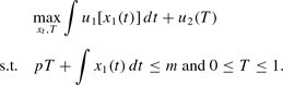
Multiple Time Periods
One of the main uses of the idea of using lotteries in a competitive system is that in Rogerson (1988). It is used there to explain the existence of unemployment. Assume that working is a zero-one decision as in Section 4. Then, as above it is optimal to allow randomization. As we have seen, it follows that the “odds” on the lottery are directly related to (exactly equal in our case) the prior probability that the agent ends up in states 0 and 1. If there are many identical agents buying identical lottery tickets that are independent, we should see (in our formulation) roughly
percent of the agents buying the indivisible good (unemploymed) and
percent not buying the good. Thus, the outcome of the lottery tickets is used to ration (in a nonprice way) the indivisible good (jobs).
A natural question to raise here is that if the time horizons we are considering are sufficiently divisible, why cannot timing perform the same function as the lotteries? Thus, if winning the lottery means spending two weeks in Hawaii (two weeks unemployed) and losing means spending those two weeks at home (working), why not spend one week at home, one week in Hawaii, and avoid the lottery altogether? Whether or not this alternative is optimal clearly depends on the costs, and so on.
Our aim here is simply to show that this affect can overturn the results of Section 4, so we will analyze a very simple continuous time model. At time 2, the agent must choose a time path of consuming some indivisible good. That is, he must choose a [x1(t), x2(t)],
to maximize U(x1, x2) subject to a budget constraint and the constraint that x2=0 or 1 (a.e. dt).
To make our point, we will assume that both U and the budget constraint are of very special forms.
Assume that
where u1 is strictly increasing, continuous and strictly concave. Assume that the budget constraint is given by

Let V*(m) be the utility at the maximizing value in this problem as it depends on m. It can be shown that a solution to this problem always exists. We have:
PROPOSITION 3
V*(m) is strictly concave.
The proof is immediate.
Notes
1. It follows immediately that although the agent will buy insurance against fluctuations in his initial income, he will not gamble.
2. The assumptions we have made are indeed very special. There is no discounting, preferences are separable between the indivisible good and the numeraire, prices are constant across time, and so on. It is clear that the crucial assumption is the form of utility in the indivisible good, however. Given our formulation, the agent does not care when he consumes the good, just how often. This allows us to transform (4) into a choice problem between x1(t) and
.
This problem is
.
Because this new problem is concave, Proposition 3 follows immediately. Thus, the intertemporal substitutability in consumption of the second good “undoes” the effect of the indivisibility by substituting percentages in time for probabilities.
Given this one might think that considering utility functions of the form
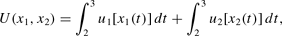
will introduce a noncavity in V*. This is not the case, however. Let
and assume that u2(0)=0. π then is the percent of time utility is spent at u2(1). We can then rewrite (4) as
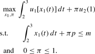
Again, this problem is concave and Proposition 3 follows. If there is discounting and/or p is not constant things are obviously trickier.
3. The essence of the argument presented here is that the form of the utility functions and/or other features of the consumption set can greatly diminish the importance of the presence of obvious nonconvexities. This criticism applies equally well to both the model in Rogerson and that presented in earlier sections. Of course, the extent to which this occurs depends on other features of the consumption set—one must fly to Hawaii and the cost of this in both time and money is independent of the amount of time spent there, one must travel to work each day, and so on. It is the presence of these other noncenvexities that is probably most important in practice.
4. The result in Proposition 3 should not be surprising. After all, time sharing and rental arrangements are a big industry. (Alternatively, lottery winners could be given sole ownership.)
Final Added Note
This last result—the fact that lotteries are unnecessary in a continuous time model—has attracted some attention of late [see Ljungqvist and Sargent (forthcoming) and Prescott (forthcoming)] and has also been studied in Mulligan (2001). So it is worthwhile noting that it can be extended beyond what is done here. In particular, it is interesting to study the role played by the assumption that there is no discounting. In this section we give one set of sufficient conditions under which V* is concave (and hence there is no social value to lotteries) even with discounting.
Consider the following household optimization problem:
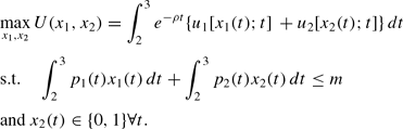
Let V*(m) denote the value of utility at the solution to this problem.
Note that for any feasible choice of x2:

That is,

where D=∫e−ρtu2(0; t) dt is a constant.
Based on this, consider the following, alternative, maximization problem:
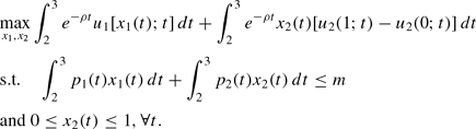
That is, we relax the assumption that x2(t)∈{0, 1} to 0≤x2(t)≤1.
Let V**(m) denote the value of the solution to this problem. It is straightforward to show that V** is concave as the first term in the objective function is concave and the second is linear.
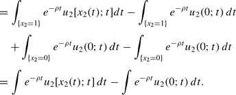
The only thing left to be shown is that there is a solution to the new problem that is also feasible for the original problem. That this is true follows from the fact that
is linear in each x2(t). Because of this a solution can be found for the problem for which x2 is bang/bang—it is either 0 or 1.
Hence, V*(m)=V**(m) for all m. Because of this it follows that lotteries are not of any value.
As a final note on this problem, it can be seen that the solution to the household's problem has the form that x2(t)=1 exactly when e−ρt/p2(t)[u2(1; t)−u2(0; t)] is maximal—if x2(t)=1 for some t, it is also 1 for any τ such that

Because the solution takes this form, it is not necessarily true that the only thing that matters is fraction of the time that x2 is 1. There is, however, one special case when this is true. This is when u2(x; t) is independent of t and e−ρt/p2(t) is a constant—basically with constant interest rates given by the rate of time preference, ρ.2
Even if u2(.; t) does depend on t, this result will still hold as long as e−ρt[u2(1; t)−u2(0; t)]/p2(t) is a constant. This would hold, for example, with equal seasonal effects in both utility and prices.
CONCLUSION
The aim of this note was to provide an alternative motivation for “effective” nonconcavities in the indirect utility function for money. This leads directly to a justification for gambling even in the presence of diminishing marginal utility (as much as this makes sense).
We also have argued that certain other natural properties (quality gradation or timing decisions) may lessen the practical importance of the essential nonconvexities.
One could plausibly argue that the existence of such mechanisms as lotteries in reality shows that these problems do exist.
Throughout this note, we have assumed that gambling does not directly give rise to utility. Alternatively, one might suppose the opposite and base a theory of the existence of lotteries in this way. This is, of course, perfectly valid. Note, however, that generally we would expect that the rich people would gamble more (if gambling is a normal good), whereas in the theory presented here the opposite would hold.
We have ignored the possibility of private information and the problems that it would cause in providing complete insurance. Although important, these issues did not seem of sufficient magnitude to justify complicating the model through inclusion.
I am indebted to V.V. Chari, E. Prescott, T. Sargent and E. Zemel for helpful conversations, the National Science Foundation for financial support, Anderson Schneider for his expert research assistance, and seminar participants at the University of Chicago for their always stimulating hospitality.