


A weak financial system—reflecting an underperforming banking system, poor investment protection and corporate governance, or fragile securities markets—yields a high cost of financial intermediation. For any given return on an investment project, savers' net return is lowered by the high cost of financial intermediation.
R. G. Hubbard, The Wall Street Journal Europe, 23 June 2005
INTRODUCTION
Traditional asset pricing models have emphasized the role of financial markets in allowing agents to transfer purchasing power over time and across states of the world. Equilibrium asset prices and rates of return are typically derived in these models as those that ensure that a representative agent has achieved the optimal intertemporal allocation of consumption given the constraint represented by his lifetime income. As a result of this simplification, in these models a number of imperfections and frictions that characterize the actual functioning of financial markets are not explicitly considered.
Asset pricing models based on the assumption that the only function of the financial markets is to transfer purchasing power over time and across states of the world certainly represent a useful benchmark, but overlook a number of additional benefits and costs that participation in financial markets entails and that are highly relevant in reality. These additional elements may include “objective” factors such as the possibility of using financial assets to purchase goods and services or, in a lending relationship, the need of undertaking a monitoring activity on the creditworthiness of the recipient of the funds in a context of asymmetric information. Moreover, “subjective” factors related to the extent to which the holding of certain assets and liabilities has an impact on agents' psychological well-being may also play an important role, as emphasized long ago by Keynes (Keynes, 19361
The reference is, in particular, to purely subjective motives for saving, such as the sense of independence and security that the holding of financial assets confers, or pure avarice, which are adequately emphasized in the General Theory (see also Browning and Lusardi, 1996).
Providing a systematic framework for evaluating the impact of these factors on equilibrium asset prices and rates of return is the main purpose of this note. The model aims at providing a general framework and a language useful for thinking about this type of issues in a systematic manner, and it is not the primary aim of the analysis to provide explicit analytical results in terms of closed form solutions.
The note is organized as follows. Section 2 presents the setup of the model and the optimization by individual households. Section 3 describes the equilibrium in the financial market. Section 4 deals with the pricing of liquidity services in equilibrium. Section 5 concludes.
THE MODEL
Basic Features
In the same way as in standard intertemporal models, we derive equilibrium real rates of return in a model in which agents solve an explicit dynamic optimization and goods and financial markets clear. However, unlike in standard models, we assume that the decision of holding financial assets and liabilities entails benefits and costs on its own, which contribute to agents' utility. This work is closely related to two thus far quite separate strands of literature. On the one hand, the model is a broad generalization of the asset pricing models with money in the utility function, for example as in Bakshi and Chen (1996).2
Tobin (1969) is an earlier classic reference on a general equilibrium approach to monetary theory.
Goods prices are completely flexible in this economy. In line with conventional assumptions, each household maximizes its lifetime utility subject to the usual budget constraint. Furthermore, for simplicity of exposition, it is assumed that households are risk neutral. This allows to abstract from risk considerations in the description of the model, which are not central to the core issues being analyzed.
Another important feature of the model is that agents are assumed to be heterogeneous along a number of dimensions, including their appreciation of the liquidity services provided by different financial assets. So, the analysis does not hinge on the restrictive and implausible assumptions needed to consider exact linear aggregation across agents and a single homogeneous representative agent, as emphasized notably by Kirman (1992).3
See also Barnett and Serletis (2000) for a review of issues related to the aggregation across heterogeneous agents.
There is a long tradition especially in financial economics in linking the concept of liquidity to the degree of asymmetric information between borrowers and lenders in financial and credit markets. For example, it has been emphasized that the liquidity of the market is inversely related to the number of privately informed traders and adverse selection problems (Bagehot, 1971). Notably, adverse selection may increase in a financial crisis, leading to a disruption of liquidity. In the model, we assume that all financial liabilities are repaid, and default is not possible.4
Note that adjusting the model to incorporate the possibility of default would not change its main features by much, as long as agency costs are taken into account in the no-default specification. So, instead of having a “lemons premium” in the model (Hubbard, 1998), we have a “cost of detecting lemons,” which is in practice not that different.
In addition to these objective factors, many benefits and costs associated with the holding of financial assets and liabilities may be related to their subjective impact on agents' psychological well-being. For example, having a fat bank account or experience stock market gains can give a sense of security and satisfaction to agents in itself, that is, in addition to the effect on consumption. Running on debt, conversely, may cause anxiety independent of the probability that the debt may, or may not, be paid back (debt aversion). These factors have long been emphasized in the literature on saving (Browning and Lusardi, 1996) and also have received some attention by behavioral economists such as Thaler (1990). According to Thaler, agents may frame certain financial assets and liabilities into separate mental accounts, which implies that different types of financial wealth are more or less convertible into transaction balances. Moreover, certain features of financial assets might help households to solve self-control problems of the type described by Laibson (1997).5
This would suggest the paradoxical conclusion that sometimes it is the apparent illiquidity of financial assets (namely the difficulty in converting them into transaction balances), which might improve their “liquidity services” as defined in this paper. This happens because illiquidity (in the traditional sense) helps agents solve their self-control problems and so results in a benefit for them (i.e., higher liquidity services). However, the use of the concept of lack of self-control should be used with some caution in this paper because we are assuming that agents are fully rational and apply standard exponential discounting.
It also should be emphasized that this study focuses on the macroeconomic equilibrium and the determination of the equilibrium interest rates in the economy. Thus, it departs from the focus traditionally maintained in the finance literature on the role of liquidity factors (such as transaction costs) in the pricing of individual asset prices (Brennan and Subrahmanyam, 1996; Pastor and Stambaugh, 2003). Moreover, the definition of liquidity is clearly broader than that traditionally assumed in the finance literature.
SetUp of the Model
Following in particular Woodford (1996), we assume that the economy consists of a continuum of infinitely lived households indexed by j in [0, 1]. Each household specializes in the production of a single differentiated good. The continuum of differentiated goods is denoted by z in [0, 1], where z=j is the good supplied by household j. As noted, there is no government, and the economy is closed.6
The basic framework can easily be extended to study government policy, as government intervention affects asset supplies and hence real rates of return.
The same consideration is valid for the government, although with probably a somewhat smaller degree of realism.
The economy includes a goods market and a financial market; prices are perfectly flexible and set competitively in both markets. In the following, p(z) denotes the price of good z, with the general price level being normalized to one. Because nominal goods prices do not play any role in determining real quantities, we will always refer to real values in the continuation of this analysis. Financial assets are exchanged in the financial market, and households can theoretically have both assets and liabilities without constraints.8
We assume that no-Ponzi conditions hold and that sustainability issues do not play any role in our economy.
the real market value, expressed in net terms, of the instrument i, with i=1, … , n, held by household j, with j=1, … , m, where
indicates a net asset, and
a net liability. It should be noted that the index i refers to both the technical characteristics of the financial instrument and the identity of the borrower (in the case of financial assets) or the lender (in the case of financial liabilities). So, for example, a financial asset i1 might be a “bank loan to Mr. X,” or a financial liability i2 might be “credit received from firm Y.”
From now on, we indicate with
a financial instrument held as an asset by household j, and
the same financial instrument held as a liability, with
. The vectors
,
and
will denote, respectively, the full set of financial assets, liabilities, and net holdings in period t by household j, and the vector with the rates of return will be denoted by
.
is the current market value of the assets and liabilities portfolio,
is the ex post market value of asset i in time t compared with time t−1. Assuming for simplicity that all assets are zero-coupon, this is the gross rate of return on asset i. Agents are assumed to be risk-neutral. For ease of exposition, the expectational term will be omitted in the continuation as it does not play any useful role in the analysis.
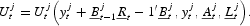
For each household j, the flow budget constraint is defined as follows:
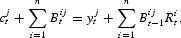
or, expressed in vector notation:
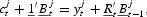
where
is the consumption of household j, including capital goods, and
where
is the output produced by household j. Obviously, expected returns are given for an individual household, but they are determined endogenously in the economy as a whole, as we shall see in Section 3.
Preferences and the Optimal Portfolio Choice of the Individual Household
The main novel element in the model is represented by agents' preferences. Each household j has the following instantaneous utility function:
where
,
,
,
(in line with standard assumptions). We do not impose any restriction on the signs of
and
, as we want to allow for the possibility that the holding of financial assets and liabilities may imply both net benefits and net costs at the margin, depending on the type of asset and the agent concerned. Irrespective of whether they are positive or negative, benefits or costs are characterized by diminishing marginal returns, which appears to be a plausible assumption in most situations. Hence, we impose that the Hessian matrices
and
are negative-definite. Note that we do not impose any form of separability in the utility function; so, the holdings of a certain financial asset or liability might in principle affect the liquidity of all other assets and liabilities, and in reality they often do. For example, the liquidity benefits of having a money market fund are greatly reduced if the agent already has a large bank account surplus.
It should be noted that the production function and the market for production factors are implicitly included in the Uj function, as they determine the quantity of output that is possible to produce for a given amount of leisure and, therefore, the optimal allocation of time between work and leisure. The utility function is indexed by j, which captures the idea that households may be heterogenous in tastes and production technology. Moreover, the utility function is indexed by t, that is, it is time-varying. This reflects the fact, for example, that the trade-off between consumption and leisure changes over time due to technical progress (which allows more production for a given amount of effort).
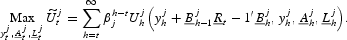
Households maximize a lifetime utility function with instantaneous utility given by (3). The expected lifetime utility function is defined as follows:
where 0<βj<1 is the discount factor of household j. Rewriting (4) taking into account the budget constraint in (2):
Hence, the decision problem of the agent is:
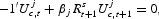
The first-order condition for
is:

and for
:
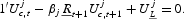
Each agent j decides his optimal portfolio of financial assets and liabilities in order to satisfy the conditions set out in (7) and (8). The only difference with a standard intertemporal model is given the liquidity terms
and
. This is evident when considering a theoretical financial asset s that provides no liquidity services either as an asset or as a liability, and only guarantees an automatic transfer of purchasing power over time.9
From the discussion in the foregoing, it should be clear that this type of asset hardly exists in the real world; it is merely an artificial construct.
As in any intertemporal model, the marginal utility associated to this type of asset is given by:
where
is the hypothetical rate of return on asset s. Therefore, considering (7), (8) and (9) jointly, we obtain that our household j chooses an asset and liability allocation
such that:
and this is valid for any asset i and household j. The intuition behind this expression is that the term on the right hand side of the equation, a measure of the user cost of asset (or liability) i, is a premium for the liquidity services provided by i as a financial asset or liability, scaled by the marginal utility of future consumption.
In order to derive the demand functions in terms of order flows submitted to a hypothetical auctioneer in a Walrasian market, we can write equations (7) and (8) as Marshallian demand functions of the real rates of return:

Generally, we cannot say anything certain on the sign of
(see Taylor, 1999), as an increase in the rate of return can have, in this model in the same way as in any model with heterogeneous agents, two opposing effects. On the one hand, the substitution effect implies that higher rates of return translate into a stronger demand for financial assets. On the other hand, for agents having a relatively large accumulated asset position a higher rate of return on a certain asset implies a positive wealth effect on expected lifetime income, which may have the opposite impact (namely lower the demand for the asset). Overall, the net effect at the household level (let alone the aggregate economy) is left indeterminate.
In any event, expression (11) cannot be directly the order flow because this has to be non-negative. Hence, the order flow for asset i by agent j,
, is given by:
And similarly for i as a financial liability:
where, again, the sign of the derivative
is in principle indeterminate.
The order flow of agent j will hinge on the traditional determinants of net borrowing demand emphasized in the traditional intertemporal models. Thus, depending on his discount factor and the degree to which his income is rising or declining through the lifetime, our agent will have a certain net borrowing demand. In addition, his order flow also will be significantly influenced by the liquidity services provided by the individual financial instruments, in this case in gross terms, namely, distinguishing between assets and liabilities. This will in turn reflect personal characteristics as well as the technological and contractual features underlying financial instruments. The end result of the combination of all these factors is the order flow equations which are shown in (12) and (13).
It also should be emphasized that, unlike in the standard approach which neglects the existence of the liquidity terms, the possibility exists that our household does not participate in the market for certain assets (or even in financial markets at all). This may happen if, for a certain agent j,
and, at the same time,
, in which case
.
This consideration suggests that the analytical framework developed here provides a simple way to model phenomena normally referred to as limited participation in the financial market. In particular, this setting should generalize the traditional limited participation assumption, i.e., that some agents are for some exogenous reason excluded from taking part in the financial market altogether, which has been often maintained in the literature (see, for example, Fuerst, 1992). On the same token, the model endogenously derives that agents may be willing to hold both assets and liabilities in their balance sheet even in the absence of risk considerations.10
The contemporaneous holding of financial assets and liabilities can of course be justified in different models, but all of them have some built-in form of heterogeneity. For example, Gertler (1999) derives simultaneous borrowing and lending in an overlapping generations model. It should be noted, however, that unlike in Gertler (1999) our model explains the possibility that the same individual holds both assets and liabilities, a point which is emphasised by Stiglitz and Greenwald (2003).
Having described the problem of the optimal selection of financial assets for an individual household for given market returns, in the next section we set out to characterize the equilibrium in the economy as a whole.
THE EQUILIBRIUM IN FINANCIAL MARKETS AND REAL EQUILIBRIUM INTEREST RATES
At the aggregate level, we impose the condition that each asset is in zero net supply, because in a closed economy with no government every financial asset for a certain household is also a financial liability for another household. We also assume the existence of a Walrasian auctioneer who matches the order flows of each individual household and is able to find a price (rate of return) for each asset so that the order flows match. Therefore, the relevant market equilibrium condition for each asset i is the following:

So, the price of asset i must ensure, for the equilibrium to be maintained, that the vector of returns,
, is such that
. This in turn implies:
or:
where we refer to
as the subset of agents who participate in the market for asset i as a financial asset (i.e., for whom
), and to
in the market for asset i as a financial liability (i.e., for whom
). This expression identifies the level of real equilibrium interest rates. It should be noted that a unique equilibrium vector, say
, ensuring that condition (16) holds exists only to the extent that, at the aggregate level, the excess demand curve,
, is strictly decreasing in the rates of return, namely,
.
A unique equilibrium is of course not warranted for any conceivable financial instrument as even at the level of the individual household the relationship between the demand for assets and liabilities and real returns is not a straightforward one, because of the existence of substitution and wealth effects, as mentioned in the previous section. So, we assume that the financial market is able to clear for a subset of the theoretically possible financial assets, and we define the set of the available financial instruments, i=1, … , n, to be the one for which a market clearing is attainable. Generally speaking, as everything in the model is time-varying, the set of financial instruments for which market clearing is feasible (and therefore a market exists at all) also will be time-varying.
It is also worth stressing that in this model the total gross supply of, and demand for, financial assets are related primarily to the heterogeneity across households, whereas market prices (expected returns) ensure that demand and supply are equalized. This is a main advantage of considering heterogeneous agents in an asset-pricing model, in that both prices and quantities may be derived.
LIQUIDITY AND REAL EQUILIBRIUM INTEREST RATES
We have now set the stage for the analysis of the pricing of liquidity services in equilibrium. This is an important matter which has been extensively dealt with in the literature on monetary aggregation (Barnett and Serletis, 2000) as well as in an earlier Keynesian literature emphasizing the role of agents' preference for liquidity in the determination of the monetary rate of interest. In the Keynesian theory of the “own rate of money interest” (see Bibow, 1998, for a review of this concept), the monetary rate of interest can be defined (simplifying) as:

where r is the real interest rate on a financial instrument,
is the real interest rate on a risk-free nonliquid asset, l is liquidity (inclusive of carrying costs), and σ is a measure of risk. Therefore, in this framework an improved liquidity of financial instruments leads necessarily to a fall in equilibrium real interest rates, everything else remaining unchanged. This view is reflected in the idea that low liquidity, for example, because of the high cost of financial intermediation, must increase the return required by savers and hence real rates of return (as evident in the quotation shown at the beginning of this note). In the present framework, however, evaluating the impact of liquidity on equilibrium real interest rates is a more complex matter on account of the heterogeneity across agents and the fact that both assets and liabilities can have liquidity services, which have to be priced in equilibrium. In particular, the important element is the extent to which the liquidity services of the financial instrument i (seen both as an asset and as a liability) impact on the excess (rather than gross) demand for it, namely
. For example, a financial instrument that is very liquid for asset holders but that is even more liquid for liabilities holders generally will have a higher rate of return compared with the benchmark liquidity-free asset (namely, a negative user cost). In other words, the general equilibrium and heterogeneous agents nature of this model leads quite naturally to look at both sides of a financial contract, given that they both matter in the determination of the equilibrium rates of return.
The Effect of Improvements in Liquidity Due to Technical and Contractual Progress
Financial and payment technological and contractual innovation may contribute over time to change the liquidity services provided by financial assets and the cost of producing them. In the Keynesian theory of the “own rate of money interest” described earlier, it might be argued that improved liquidity should contribute to reducing real equilibrium interest rates over time. This conclusion, as noted, is not necessarily warranted in a framework with heterogeneous agents and asymmetry in liquidity services between assets and liabilities as the one proposed in this note. Notably, we should entertain the possibility that technological and contractual innovation also affects the liquidity services and costs for financial liabilities. For example, in most industrialized countries, a debtor cannot be imprisoned anymore if he fails to pay back his debt. It can be argued that this type of legislative progress increases the liquidity services provided by all financial liabilities, and should ceteris paribus result in higher equilibrium real interest rates. Another interesting example is technological innovation in the banking sector. Suppose that agents are better able to monitor their bank accounts as a result of, say, the home banking technology. This factor, in itself, raises the demand for these assets and hence the real equilibrium rates of return on them. By contrast, however, suppose that banks become better able to track movements in the current accounts of the customers, implying an improved liquidity of the liabilities side of their balance sheet. The net effect of this type of innovation will depend on the effect on the liquidity and therefore the desired holdings of assets and liabilities of each agent, which makes—in an heterogeneous agents model—the aggregate effect extremely uncertain.
Real Equilibrium Interest Rates in a Financial Crisis
Let us now turn to the conceptually opposite case when unrest in financial markets leads to an exacerbation of agency costs and to lower liquidity. Trust between borrowers and lenders is eroded in these hard times. This is a situation that has been amply emphasized in the literature, where the financial system is thought to be unable to channel funds to those with the best investment opportunities (Mishkin, 1991) and information asymmetry problems deepen, leading to illiquidity (Glosten and Milgrom, 1985). Reflecting this view, the traditional reaction of central banks to financial unrest has been to provide highly liquid instruments (i.e., cash) to the market, notably through their lender of last resort function.
What happens to real equilibrium interest rates when markets become more illiquid? In the traditional Keynesian view, this translates into a lower l and this implies higher real interest rates in equilibrium, as evident from equation (17). However, it should now be clear from the previous discussion that the evaluation of the overall impact of an increase in agency costs onto real equilibrium interest rates is more complex than the Keynesian view suggests. Again, what matters is the impact of these developments on the excess, rather than gross, demand for each financial instrument, that is,
(and not
). For example, depending on the nature of financial contracts and the incentives faced by borrowers and lenders, an increase an agency costs may result in reduced liquidity for both asset holders (in terms of higher screening and monitoring costs) and for liability holders (in terms of signaling). The net effect of these factors onto equilibrium asset returns, also taking into account the heterogeneity across households and the aggregation biases that it implies, is once more far from straightforward.
In particular, it will be important to have a close look at the relative situation of debtors and creditors in the economy. This is especially relevant if, as is often the case in advanced economies, debtors and creditors in the economy typically belong to distinguished and well-identified sectors (for example households and corporations). In this situation, a problem originating in a certain sector (say in the households sector) might have a considerably different impact on the level of the natural rate compared with the same problem experienced in another sector (say nonfinancial firms). Overall, the model presented in this note provides a useful analytical framework to think in a rigorous way about this kind of issues, also from a policy perspective.
CONCLUSIONS
This note has proposed a simple general equilibrium intertemporal model with heterogeneous households and a financial market in which each financial instrument provides liquidity services in addition to the property of transferring purchasing power over time. The model proposes a view of the equilibrium real interest rates that reflects the traditional determinants (such as time preference and technology) but also the liquidity services provided by the financial assets and liabilities.
The analytical framework introduced in this note appears to be particularly suited to study situations in which “liquidity matters,” and that the traditional intertemporal models are not able to address satisfactorily. In this note, we study the determination of equilibrium real interest rates when financial innovation improves the liquidity services provided by financial instruments, or alternatively when a financial crisis leads to a drying up of liquidity.
The framework proposed in this note appears to provide a simple and useful setting to model, and a language to talk about, a series of imperfections and frictions in financial markets which are difficult to deal with in a simple manner in standard intertemporal models. Moreover, the model seems particularly appropriate to study issues related to heterogeneity that are normally set aside.11
Of course, this is not to say that limited participation in financial markets and heterogeneity have not been already dealt with altogether in the literature. For example, Brav, Constantinides, and Geczy (2002) provide a very interesting analysis of the role of limited participation and incompleteness in financial markets in a heterogeneous agents economy.
Clearly, the analysis in this note is only a first step and could be extended in several directions. Physical assets and open economy considerations could be explicitly included in the model, to have a more complete picture of the determination of equilibrium real interest rates under flexible prices in a realistic economy. Moreover, the role of risk and risk aversion might be integrated relatively straightforwardly in this framework. Finally, in this model we have assumed that liquidity services enter in the utility function with diminishing absolute marginal returns, but it is not difficult to envisage situations in which liquidity may be characterized by increasing absolute marginal returns. For example, an agent's debt aversion and therefore the marginal disutility associated with debt may actually increase, the larger the financial liability position in absolute terms. Studying the effects of absolute increasing returns may be intriguing because it is likely to endogenously give rise to nonconvexities possibly leading to quantity rationing that have been emphasized in the information economics literature (Stiglitz, 1999).
I thank Bill Barnett, the editor, and two referees for several useful comments. A more extended version of this note is available as European Central Bank working paper n. 542, available at www.ecb.int. The views expressed in this paper are those of the author and are not necessarily shared by the ECB.
