INTRODUCTION
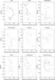
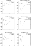
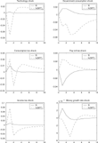
Looking at U.S. data, the relationship between the money-to-income ratio and the nominal interest rate is quite stable and clearly negative. This seems to confirm not just conventional wisdom but also traditional models of money demand [see Cooley and LeRoy (1981) for a good, and critical, survey]. Looking at Swedish data, however, we find that the relationship is weakly positive. Moreover, a survey of 18 different OECD countries exhibits a wide range of patterns (see Figures 1 and 2). Some countries, such as Iceland and Switzerland, are similar to the United States. Others, such as Great Britain and Portugal, look more like Sweden. Prima facie, this looks like a challenge to traditional theoretical models.

ln(M/Y) versus R in nine OECD countries.

ln(M/Y) versus R in nine other OECD countries.
In this study, we show that this challenge can be met by using the standard tools of the neoclassical tradition. If one takes into account the fact that Swedish and U.S. economies have been hit by different shocks, the basic properties of the data on money and interest rates can be accounted for reasonably well.
This result might seem counterintuitive. Indeed, several monetary equilibrium models in the literature, for example, Sidrauski (1967) and Lucas and Stokey (1987), have the property that a deterministic negative relationship between real balances and the nominal interest rate can be derived, and this relationship is independent of the precise nature of the shocks that hit the economy. And even if we would find a model that did not have this property, surely any reasonable model exhibits a negative relation between money and interest rates across steady states. Actually, so do the model we consider here. But comparative steady state relations can be an unreliable guide to the relationships we should expect to find in time series. In the model in this study, the time-series relationship between money and interest rates turns out not to be deterministic but to depend on the relative volatility of the various shocks.
The overall strategy of this study is the following. Treating technology, monetary policy, and fiscal policy as an exogenous vector autoregression (VAR) process, we estimate this process as a VAR using least-squares. Taking this VAR process as given, we fit a monetary general equilibrium model to the data in two different ways. First we take our preference and technology parameters “off-the-shelf”; that is, we use parameter values that have been used in the literature, using the same values for both the United States and Sweden. Second, we formally estimate our model using a combination of the generalized method of moments (GMM) and the simulated method of moments (SMM), a method that also allows us to test the model's implied moment conditions.
The main result is that the model does well in capturing the differences in the money to income and interest rate relationships in the United States and Sweden. An informal look at the empirical and simulated data reveals that the model is able to reproduce the main features of the relationship. In particular, the model is able to reproduce the differences between the two countries in a striking fashion. That is, the model produces a stable and negative relationship for the United States, whereas it produces a weakly positive relationship for Sweden. Formally, we find that none of our models can be statistically rejected, although we concede that the power of our tests may be low.
We find that the character of this relationship is determined partly by preference and technology parameters but mainly by the differences in the shock processes that have hit the two economies. Technology shocks alone create a near vertical relationship in both countries since those shocks hardly generate any volatility in the nominal interest rate. Adding on money growth rate shocks create a stable and negative relationship in the United States, whereas in Sweden they create only a weak negative relationship. There are two main reasons for this. In the United States, money growth rate shocks have been relatively more persistent than in Sweden. But, more important, money growth rate shocks and technology shocks are positively correlated in the United States, whereas they are almost uncorrelated in Sweden. Whenever money growth is high, technology also will be high. Higher technology increases output, which enhances the fall in the money-to-income ratio. This makes the relationship between the money-to-income ratio and the interest rate steeper in the United States than in Sweden. The main effect of adding on shocks to fiscal policy is to increase the variance of the interest rate and of the money-to-income ratio in both countries, which brings the relationship closer to what we see in the data.
The study is organized as follows. In Section 2, we present the facts that we would like to explain. Section 3 presents the dynamic general equilibrium model that we use to try to explain these facts. In Section 4, we report the results from the simulations of our model, and Section 5 concludes.
THE FACTS
The United States
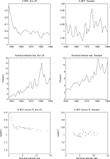
Using annual data from 1947 to 1990, the relationship between the natural log of the money to income ratio and the nominal interest rate is depicted in Figure 3. The regression coefficient is −1.95, the sample standard deviation of the interest rate is 0.030 and the sample standard deviation of the log of the money-to-income ratio is 0.094.

Money/income ratios and interest rates in the United States and Sweden.
Sweden
Using annual data from 1950 to 1990, the relationship between the natural log of the money-to-income ratio and the nominal interest rate is depicted in Figure 3. The regression coefficient is weakly positive; that is, 0.49 with a standard error of 0.31. Hence, the regression is not significantly different from zero. The sample standard deviation of the interest rate is 0.024 and the sample standard deviation of the log of the money-to-income ratio is 0.049.
THEORETICAL FRAMEWORK
On top of a standard real business cycle model with adjustment costs for capital we impose a shopping time (ST) technology in order to create a role for money. The model is driven by stochastic shocks to technology, government spending, taxes, and the money supply. These shocks are modeled as VAR processes.
The main nonstandard feature of the model is the presence of stochastic fiscal and monetary policy. There are several reasons for including stochastic policy. In the first place, it adds realism in a way that we know is important. That stochastic policy increases the empirical fit of business cycle models has been established for the United States by McGrattan (1994), Braun (1994) and others, and for Sweden by Jonsson and Klein (1996). Also, because the empirical relationship between money and interest rates differs significantly between the United States and Sweden, it makes sense to build into the model those observables that might explain these differences, and the different policy processes are natural candidate explanations. In order to capture the differences between the policy processes to the extent that we need, it seems necessary to include not just differences in first moments but in variances and autocovariances as well. This requires the assumption of stochastic policy, and immediately suggests a (linear) VAR specification because such a specification not only captures variances and autocovariances well but also easily fits into a linear rational expectation framework.
The tax systems are modeled in slightly different ways for Sweden and the United States. The main reason for this is the availability of data. For example, there exists no good time-series on Swedish tax rates that distinguishes between labor and capital income taxes. By contrast, we do have good data on the Swedish payroll tax rate, which only affects labor (and not capital) income.
Households
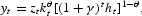
The economy is inhabited by a large number of households. A representative household has preferences,
, over stochastic processes for consumption, c, and leisure, [ell ], according to
where t denotes time, E the unconditional expectation operator, U(·) the utility function, and β∈(0, 1) the subjective discount factor. The period utility function has the standard iso-elastic form
where α ∈(0, 1) measures the weight on consumption relative leisure, σ denotes the coefficient of relative risk aversion and 1/σ the intertemporal elasticity of substitution.
In the model adapted for the United States, the budget constraint, in real terms, is given by
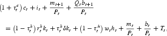
where mt denotes the amount of money carried over from period t−1 (and held at the beginning of period t), mt+1 the amount of money carried over into period t+1 (and held at the end of period t), Qt the money price of a nominal bond that delivers one unit of currency in period t+1, bt the quantity of bonds carried over from period t−1 and that mature in period t, bt+1 the quantity of bonds carried over into period t+1, kt the physical capital stock, it the investment expenditure, ht the fraction of time spent in paid employment,
the rental rate of capital, wt the wage rate, Pt the general price level; that is, the money price of goods,
the consumption tax rate,
the labor income tax rate,
the capital income tax rate and δ the depreciation rate, which is modeled as tax deductible. The (real) transfer payments from the government is denoted by Tt, some (but not necessarily all) of which may be in the form of currency. For the model adapted to Sweden, the corresponding constraint is
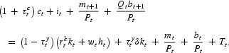
where
denotes the general income tax rate. Throughout this paper, capital letters denote aggregated per capita variables and lowercase letters denote individual decision variables. For prices, that is,
capital letters denote nominal prices and lowercase letters denote real prices.
A role for money is introduced through a shopping-time technology, which is a simple way to model the fact that money facilitates transactions. The functional form for the shopping-time technology follows Ljungqvist and Sargent (2000):
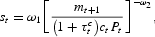
where st denotes the fraction of time spent “shopping” and ω1 and ω2 are parameters. Note that bonds (even when they have matured) cannot be used for shopping. If they could, there would be no role for money in the model. What distinguishes nominal from real bonds is that their real value in terms of goods depends on the general price level in the period of maturity.
To model the idea that capital equipment may be costly to install we introduce adjustment costs for changing the capital stock. The adjustment costs are assumed to be quadratic and zero in steady state and the functional form is taken from Chari, Kehoe, and McGrattan (2000). Hence, capital evolves over time according to
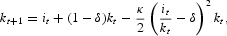
where κ quantifies the cost of changing the capital stock.
Finally, the households have a time constraint given by

where the total time endowment is normalized to one.
Firms
A representative firm rents capital and employs labor in order to maximize period profits, taking factor prices as given; that is,
The production technology is Cobb-Douglas, which means that output is produced according to the following formula
where γ denotes the real growth rate, θ the capital's share of output and zt the technology level.
The rental rate of capital and the wage rate are determined competitively as the marginal products of capital and labor, respectively. For Sweden, we also impose a compulsory social insurance contribution rate,
which drives a wedge between the wage rate and the marginal product of labor in the following way

Government
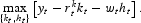
The money supply,
is determined by the following law of motion

where ut denotes the growth rate of the money supply. The growth rate is in turn determined by the following rule
where
denotes the steady state money growth rate, πt the inflation rate, and
an exogenously given money supply shock defined as
. The endogenous part of monetary policy consists of reactions to deviations of inflation from steady state and the growth rate of output. The degree of responsiveness is determined by the parameters ψ1<0 and ψ2>0. Evidence supportive of monetary policy accommodating output fluctuations can, for example, be found in Finn (1999) and Gavin and Kydland (1999). Ireland (2003) finds empirical evidence for also including reactions to inflation deviations from steady state.
The government's real budget constraint in the model adapted to the United States is

where Gt denotes government consumption and
the quantity of bonds supplied by the government at the end of period t, whereas for the model adapted for Sweden it is
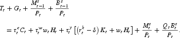
This implies that Tt is determined residually (and hence endogenously), whereas all other government policy variables are exogenous.
In addition to the notation introduced earlier, we will use Rt=1/Qt−1 to denote the one-period nominal interest rate.
The Exogenous Shock Processes
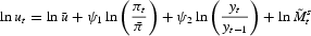
We will consider three different cases; in the first, there are shocks only to technology, in the second to technology and money growth, and in the final case we allow for shocks to fiscal policy as well. In each case, we perform a separate estimation of the resulting VAR-model. However, the mean of the shocks is fixed to the sample mean in each of the three cases. The following VAR-model is estimated

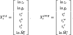
In the final case with all the shocks, Xt consists of the following variables for the United States and Sweden:1
Since government consumption is nonstationary, we use the ratio of government consumption to GDP, which is denoted by gt.
The parameters μ, φ, and Σ are estimated using least-squares. For simulation purposes, we need to construct disturbance vectors with the estimated Σ as their variance matrix. For that purpose, we multiply standard normal vectors by the matrix Ψ where Ψ is the lower triangular Cholesky decomposite of the estimated Σ matrix.
For purposes of interpretation, it is worth considering the unconditional variances and unconditional autocorrelations of the elements of the two estimated shock processes (see Table 1). Overall, we see that the Swedish economy has been hit by more volatile shocks than has the United States, and that monetary and fiscal policy has been much more volatile relative to technology in Sweden than in the United States.

Equilibrium and Solution Algorithm
We assume a competitive equilibrium in which behavior is identical across households and across firms. This allows us to treat the economy as comprising of a representative household and a representative firm. An equilibrium consists of prices and quantities, such that:
- Each household chooses consumption, investment, capital, leisure, labor, bonds, and money holdings to maximize its expected lifetime utility subject to its constraints and given government policy.
- Each firm chooses capital and labor to maximize profits subject to its constraints and given government policy.
- The government satisfies its budget constraint.
- In addition to aggregate consistency, the aggregate resource constraint hold and markets clear; that is,


To ensure the existence of a time-invariant decision rule, all variables must be stationary. For the real variables, we assume that technological growth follows a geometric trend at rate γ and proceed in the manner of Hansen and Prescott (1995).2
This procedure implies that the effective discount factor is not β but (1+γ)α(1−σ)β. Abusing the notation somewhat, the letter β will be used below to denote this effective discount factor.
SIMULATION RESULTS
How to choose the technology and preference parameters of business cycle models has been the subject of some controversy [see Hansen and Heckman (1996) and Kydland and Prescott (1996)]. In this study, we identify and implement two different ways of choosing parameters.
The first method is to take preference and technology parameters “off-the-shelf”; that is, to use the same parameters as others in the literature have done. The main advantage of this approach is that it enables us to identify the source of the different predictions for Sweden and the United States as the differences in the shock processes rather than differences in the technology and preference parameters. This means that our explanation of the facts is in terms of observable shocks rather than unobservable parameters.
The second method is to estimate some of the parameters separately for each country using a combination of GMM and SMM. One advantage with this method is that, if the weighting matrix is chosen optimally, less weight is given to uncertain moments. Also, if there are more moments than parameters to be estimated, the method provides us with a way of formally testing the hypothesis that the model's moments are equal to the corresponding empirical moments.
Off-the-Shelf Parameters
The parameter values are summarized in Table 2. Many of these values can be considered as standard since they have appeared in many studies, see for example Cooley and Prescott (1995) and Christiano, Eichenbaum, and Evans (2005). In particular, the values for α, β, γ, δ, θ, and σ are simply taken from these studies. This imply, among other things, that we set σ = 1; that is, we are assuming log-utility. The real growth rate, γ, is set equal to 0.02, which is close to the average growth rate in both countries over the period. For the capital adjustment cost parameter, κ, the parameters in the shopping time technology, ω1 and ω2, and the parameters in the monetary policy rule, ψ1 and ψ2, it is not possible to pick standard values from the literature because these values varies between different models. We choose them in the following way: κ, ω1 and ω2, are adjusted simultaneously in order to match the following three moments

where σ denotes the standard deviation and μ the mean (abusing the notation somewhat). It is not possible to exactly match these moments to the data because we restrict the parameters to be the same for both countries. Nevertheless, we succeed in matching these moments fairly well in both countries except for the standard deviation of the money-to-income ratio in the United States, which is somewhat too low in the model compared to the data. The values for the parameters in the money supply rule are taken from the estimates given in Jonsson and Palmqvist (2003). This means that the value for ψ2 is well in the range of plausible values considered by Finn (1999).
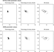
Turning now to the results for the United States, Figure 4 shows the simulated relationship between the log of the money-to-income ratio and the nominal interest rate under different shock processes. We first consider only technology shocks. In this case the variability of the interest rate almost vanishes, which induces a near-vertical relationship between the money to income ratio and the interest rate. Adding on monetary shocks, the simulated regression coefficient becomes negative and the variance of the interest rate increases. In the final case, where we also add on shocks to fiscal policy, the variance of both the interest rate and the money-to-income ratio increases. Hence, bringing the relationship closer to what we see in the data.

Simulated results, the United States.
Table 3 reports a number simulated moments related to the money-to-income ratio and the interest rate together with their empirical counterparts. All shocks are included in the VAR-model when we calculate the simulated moments. The table also reports standard errors and a simulated 90% confidence interval. The simulated regression coefficient is −3.21, whereas it is −1.95 in the data. The standard error is fairly high, which implies that the empirical value is within the 90% simulated confidence interval. The model is also close to replicate the correlation coefficient: the empirical value is −0.61, whereas the simulated value is −0.79.

The overall picture is that the model does a fairly good job in replicating the other moments as well. However, the model fails to replicate the standard deviation of some of the variables. In particular, we have difficulties in reproducing the volatility of the interest rate relative to that of the inflation rate, and this problem seems unfortunately to plague this class of models generally [see den Haan (1995).3
See also Hornstein and Uhlig (2000) for a possible way to overcome this problem.
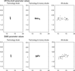
The results for the Swedish economy are found in Figure 5 and Table 4. Technology shocks give rise to a similar relationship as in the United States. In contrast to the U.S. case, adding on shocks to the money growth rate only creates a weak negative relationship between the money-to-income ratio and the interest rate. When we add on shocks to fiscal policy, these shocks increase the variance of both the money-to-income ratio and the interest rate, whereas they have a small effect on the slope.

Simulated results, Sweden.

The simulated regression coefficient is −1.14 with a 90% simulated confidence interval between −2.33 and 0.77. The empirical value of 0.49 is thus within this interval. Regarding the other moments reported in Table 4, it is notable that the model is close to reproduce the standard deviation of the money-to-income ratio and that the standard deviation of the interest rate is within the simulated confidence interval.4
Note that the model does not replicate the average nominal interest rate of about 6 percent in the data. The reason is the following: the money growth rate has been almost 9 percent in the data, which implies an average inflation rate of almost 7 percent in our model (after deducting the real growth rate). This implies that the average real interest needs to be −1 percent to replicate the nominal interest rate; that is, the subjective discount factor needs to be larger than 1. We find this implausible and therefore neclect this apparent puzzle in the Swedish data. Hence, we use the standard value for the discount rate.
SMM Parameters
In this subsection, we formally estimate the model using a combination of GMM and SMM (see Appendix B for a formal description). The parameters we estimate are the adjustment cost parameter, the parameters in the shopping-time technology, and the parameters in the monetary policy rule; that is, the following five parameters: κ, ω1, ω2, ψ1, and ψ2. For the other parameters, that is, α, β, γ, δ, θ, and σ, we use the same values as in the off-the-shelf case, as these values can be considered as standard.5
By construction, all our simulated series are stationary. Some of the empirical ones are not, however, because of real secular growth. Since the calculation of first and second moments requires stationarity in order for them to be well-defined, we filter some of the variables (both empirical and simulated) before estimation. In particular, a linear trend is subtracted from ln Yt and ln(Mt/Pt). The remaining series are left unfiltered.
The parameter estimates are reported in Table 2. The values are somewhat different compared to the off-the-shelf case, for example, the capital adjustment cost parameter is now zero for the United States, whereas it is 3.90 for Sweden. Overall, the model's moment conditions cannot be rejected neither for the United States nor Sweden (see Tables 3 and 4).
For details of the results, see Tables 3 and 4 as well as Figures 4 and 5. The results are quite similar to the case with off-the-shelf parameters. However, the overall fit of the model is better for both countries. This is because we now choose some of the parameters in order to make the model replicate the empirical moments. For example, the regression coefficient is closer to the data, both in the United States and in Sweden. In the Swedish case, the coefficient is in fact weakly positive as in the data. The confidence interval is still large, however. The reason the model does not exactly replicate the regression coefficients is because of the uncertainty associated with this moment, which leads to a low weight being given to it in the estimation.
How to Understand the Results
We report the response of the money-to-income ratio and the nominal interest rate to a one standard-deviation shock to the exogenous variables (see Figures 6 and 7). This enables us to better understand the mechanisms behind the results. The response of the nominal interest rate is shown with a solid line and the money-to-income ratio is shown with a dashed line.

Impulse responses, the United States.

Impulse responses, Sweden.
We have seen that technology shocks give rise to a near-vertical relationship between the money-to-income ratio and the interest rate. The impulse response to a positive technology shock illustrates this finding. Increased technology induces a negligible effect on the interest rate.6
This is because investment responds to the technology shock and smooths the interest rate through diminishing returns to capital.
Shocks to the money growth rate imply a negative relationship between the money-to-income ratio and the interest rate. The money growth rate is persistent, so a positive shock to it tends to increase inflation expectations and hence the nominal interest rate. And because the nominal interest rate represents the opportunity cost of holding cash, there is a tendency for agents to substitute out of money when the interest rate is high and into it when it is low. Hence, when the nominal interest rate is high because of a money growth shock, the ratio of money-to-income falls. This mechanism leads to a negative relationship between the money-to-income ratio and the nominal interest rate when the model economies are exposed to money growth shocks.
We have seen that adding shocks to the money growth rate imply a steeper slope in the United States than in Sweden. To understand this result, it is necessary to note how the money growth rate shock is correlated with the other exogenous shocks. In the U.S. data, shocks to the money growth rate and technology are positively correlated, whereas they are almost uncorrelated in the Swedish data. This means that when money growth is high in the United States, technology also is high. As a consequence of higher technology, output increases, which decreases the money-to-income ratio further. Hence, the slope will be steeper with U.S. shocks than with Swedish shocks. Another but quantitatively less important reason is that shocks to the money growth rate are more persistent in the United States than in Sweden (see Table 1).
Regarding fiscal policy, it is tempting to argue that its effect is ambiguous, leading to a more chaotic relationship whenever it is volatile. This is to some extent also borne out by the impulse responses. However, shocks to government consumption are an exception. They unambiguously lead to a negative relationship. The reason is the following. An increase in government consumption leads to lower private consumption. This causes the price of real government bonds to fall, which also leads to cheaper nominal bonds. This implies a higher nominal interest rate. Because the nominal interest rate is the opportunity cost of holding cash, real money balances falls. Output initially rises as a result of higher government consumption, but because both private consumption and investment falls, output also falls in the following periods.7
The effect of a government consumption shock on investment is ambiguous in general, but in our model the effect turns out to be negative.
In general, shocks to the tax rates lead to weak correlations between the money-to-income ratio and the interest rate. In particular, the effect depends on how shocks to the tax rates are correlated with other shocks in the VAR-model. That is why, for example, a shock to the consumption tax rate looks quite different in the United States compared to Sweden. It turns out that the main quantitative effect of shocks to the tax rates is to increase the variance in both the money to income ratio and the interest rate. Because tax rates are more volatile in Sweden than in the United States, this effect is more pronounced in Sweden. The impulse responses still suggest that, in the Swedish case, shocks to the consumption and income tax rates induce a weak positive correlation. For the United States, by contrast, shocks to each of the taxes on their own imply a weak negative relationship between the money-to-income ratio and the nominal interest rate.
In summary: The reason the model predicts a stable and negative relationship between the money-to-income ratio and the interest rate in the United States is that (i) it has been hit by shocks to the money growth rate that are positively correlated with technology shocks, which gives rise to a clear negative relationship; and (ii) it has been hit by shocks to the tax rates that induce a small negative impact on the relationship. The reason the model predicts no relationship or a weakly positive one in Sweden is that (i) shocks to the money growth rate induces only a weak negative relationship and (ii) shocks to the consumption and income tax rates lead to a weakly positive relationship.
CONCLUSIONS
In the United States the relationship between the money-to-income ratio and the nominal interest rate is a negative and stable one, while in Sweden there is no such stable relationship. We have argued that the basic neoclassical growth model is able to account for the differences between Sweden and the United States if we take into account that the two countries have been hit by different shocks. The pattern has been clear. Technology shocks alone do not generate enough variance in the nominal interest rate to create much of a relationship at all. Money growth rate shocks, on the other hand, can, and tend to create a stable and negative relationship. And we have seen that the magnitude of the slope is smaller in the model driven by Swedish shocks than in those driven by U.S. shocks. Finally, shocks to fiscal policy tend to increase the volatility of both the money-to-income ratio and the interest rate, which brings the models closer to the data.
This paper has focused on differences in the exogenous shock processes in the two countries; that is, technology, monetary and fiscal policy shocks. We have thus neglected other explanations that could be of interest. For example, Sweden is a small open economy and has therefore also been subject to foreign shocks. We have not formally modelled any credit market frictions, although the capital adjustment cost could be interpreted as a reduced form for that. Still, extending the model with a formal credit market is presumably an interesting area for future research. The framework developed by Carlstrom and Fuerst (1997) may be useful for this purpose. Other frictions, like price and wage stickiness, could also be interesting to study since they may have been different in Sweden and the United States.
APPENDIX A DATA
The OECD data is taken from the OECD publication Main Economic Indicators, various years.
UNITED STATES
The data on the money supply (M2) from 1947 to 1958 are from Friedman and Schwartz (1982). From 1959 onward, we use data from the Federal Reserve Bank of St. Louis. Because these sources contain monthly data, we take annual averages.
For the price level, we use the CPI series from the Federal Reserve Bank of St. Louis.
For nominal interest rates, we use the three-month treasury bill rate. Also, the monthly data are averaged in order to get annual data. Again, the source is the Federal Reserve Bank of St. Louis.
For government consumption, we use Citibase series GGE (nominal) and GGE82 (real). For private investment, we use the sum of GIF and GCD for the nominal series and the sum of GIF82 and GCD82 for the real series.
For private consumption, we use the sum of GCN and GCS and the sum of GCN82 and GCS82, respectively.
Income (whether nominal or real) is measured as the sum of private investment, government spending, and private consumption. This excludes increases in stocks and net exports and hence ensures that the identity Y=C+I+G holds both in the data and the model.
Data on government debt are taken from Citibase, variable FBD. This series contains the gross debt of the federal government. Ideally, one would want data on the net debt (or assets) of the consolidated government, but such data are more difficult to construct.
Data on hours worked are taken from the Citibase variable LHOURS.
In order to get per capita values, we divide by the population as measured by the Citibase variable P16.
Data on capital and labor tax rates where given to us by Ellen McGrattan. The consumption tax rates where constructed by us, using the method proposed by Mendoza, Razin, and Tesar (1994).
SWEDEN
See Jonsson and Klein (1996) and Klein (1995) for details on the collection and calculation of the Swedish tax rates. The data on the money supply (M2) was provided by Lars Jonung. For nominal interest rates, we use the Central Bank Discount Rate, Statistical Yearbook, Central Bank of Sweden. All other variables are taken from the annual Swedish national accounts, Central Bureau of Statistics, Stockholm, various years.
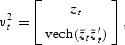
APPENDIX B TWO-STAGE GMM/SMM ESTIMATION
The following treatment is based on, but very slightly extends, the work of Lee and Ingram (1991) and Yaron (1996).
Suppose we have an empirical sequence
and K independent simulated sequences
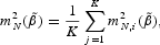
i=1, 2, …, K. Define
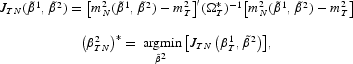
and let n be constant whenever we let T and NK simultaneously tend to infinity. Suppose we find it convenient to estimate the parameters in two stages, where the first stage uses GMM and the second SMM. Formally, define
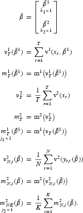
Now suppose things are constructed so that (some model implies that), for some unique β,
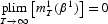
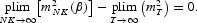
This motivates the following estimator of β (the two-stage GMM/SMM estimator).
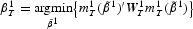

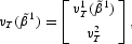
where
and
are positive definite whose probability limits W1 and W2 are non-stochastic and positive definite. The subscript T indicates that these matrices may depend on the empirical observations. An alternative, which we ignore here for reasons of convenience, is to let the weighting matrix depend on simulations instead [see Yaron (1996)].
Subject to regularity conditions, this guarantees consistency. For asymptotic efficiency, we must choose
and
optimally. The optimal choice of W1 is well described elsewhere [see, for example, Yaron (1996)].
The optimal choice of W2 satisfies

Hence, our job is to find the asymptotic variance matrix of
In order to do that, we begin by defining
(and similarly for other vectors of moments) and suppose that
Then we use our observations of
to estimate S by ST. Now define Ω via

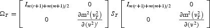
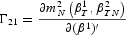
Now, if m is smooth, we have a consistent estimator of Ω in
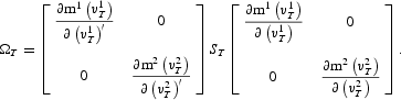
Finally, our desired variance matrix can be shown to be consistently estimated by
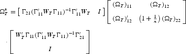
Now, because Γ21 is a function of the second stage parameters, we get a circularity problem, which is solved in some standard way. See later for one option.
A SPECIAL CASE: THE FIRST STAGE IS EXACTLY IDENTIFIED
If j1=k1 then Γ11 is square (but not necessarily symmetric) and if the first-stage moments really identify the first-stage parameters, then it is also invertible (with probability 1). Hence, our variance matrix reduces to

A Special Case of the Special Case: The First Stage is a Regression
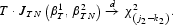
This is, of course, the case we consider in the main text. There we have an empirical sequence

and K independent simulated sequences
We will drop the superscripts e and s. Instead, subscripts T and N will represent empirical and simulated moments, respectively.
Now we partition
For convenience, define, for any sequence
,

and set

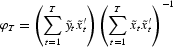
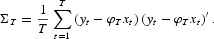
Next we define
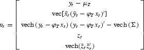

and estimate, using the formula of Newey and West (1987), the asymptotic variance matrix of
. Call that matrix S and its estimator ST. Then we partition according to
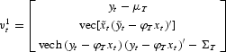
and define


Next we define

(Note that Γ11 is symmetric in this case.) Then we define

(
being defined in the obvious way) and

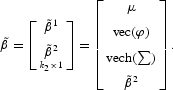
Next we define (and calculate using numerical derivatives)
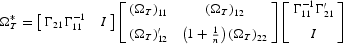
and, finally
As noted earlier, we need estimates of the second stage parameters in order to find the derivatives that are used to construct the optimal weighting matrix. To find consistent estimates of β2 for this purpose, we use the identity matrix as the weighting matrix rather than the optimal one. Given these parameter estimates, we then calculate the optimal weighting matrix and estimate β2 once more.
We are grateful to Lars Ljungqvist, Lee Ohanian, Torsten Persson, Kjetil Storesletten, Lars E. O. Svensson, and Paul Söderlind, as well as seminar participants at the Federal Reserve Bank of Minneapolis and the European University Institute in Florence for useful discussions and comments. We also are grateful to an anonymous referee for many helpful and constructive comments. The views expressed in this paper are those of the authors and should not be interpreted as the views of Sveriges Riksbank.