


1. INTRODUCTION
Considerable attention has been given in recent years to the problem of thin foil targets irradiated by high intensity laser pulses. Under these conditions a solid target transforms very rapidly, in a few cycles of the light wave, into plasma. During the short period of the laser pulse, the laser interacts directly with plasma with density on the order of the density of the solid. If the intensity of the wave is sufficiently high to make the oscillation of the electrons relativistic, interesting interactions between the wave and the surface of the plasma take place. Promising applications in a variety of areas in physics (Snavely et al., Reference Snavely, Key, Hatchett, Cowan, Roth, Phillips, Stoyer, Henry, Sangster, Singh, Wilks, MacKinnon, Offenberger, Pennington, Yasuike, Langdon, Lasinski, Johnson, Perry and Campbell2000; Robson et al., Reference Robson, Simpson, Clarke, Ledingham, Lindau, Lundh, McCanny, Mora, Neely, Wahlström, Zepf and McKenna2007; Cao et al., Reference Cao, Uschman, Zamponi, Kampfer, Fuhrmann, Forster, Holl, Redmer, Toleikis, Tschentscher and Glenzer2007; Borghesi et al., Reference Borghesi, Kar, Romagnani, Toncian, Antici, Audebert, Brambrink, Ceccherini, Cecchetti, Fuchs, Galimberti, Gizzi, Grismayer, Lyseikina, Jung, Macchi, Mora, Osterholtz, Schiavi and Willi2007; Cerchez et al., Reference Cerchez, Jung, Osterholz, Toncian, Willi, Mulser and Ruhl2008; Akli et al., Reference Akli, Hansen, Kemp, Freeman, Beg, Clark, Chen, Hey, Hatchett, Highbarger, Giraldez, Green, Gregori, Lancaster, Ma, MacKinnon, Norreys, Patel, Pasley, Shearer, Stephens, Stoeckl, Storm, Theobald, Van Woerkem, Weber and Key2008; Laska et al., Reference Laska, Jungwirth, Krasa, Krousky, Pfeifer, Rohlena, Velyhan, Ullschmied, Gammino, Torrisi, Badziak, Parys, Rosinski, Ryc and Wolowski2008; Yogo et al., Reference Yogo, Daido, Bulanov, Nemoto, Oishi, Nayuki, Fujii, Ogura, Orimo, Sagisaka, Ma, Esirkepov, Mori, Nishiuchi, Pirozhkov, Nakamura, Noda, Nagatomo, Kimura and Tajima2008) and medicine (Bulanov et al., Reference Bulanov, Brantov, Bychenkov, Chvykov, Kalinchenko, Matsuoka, Rousseau, Reed, Yanovsky, Krushelnick, Litzengerg and Maksimchuk2008; Salamin et al., Reference Salamin, Harman and Keitel2008) have been discussed and demonstrated, and in ion-driven fast ignition (Fernandez et al., Reference Fernandez, Honrubia, Albright, Flippo, Gautier, Hegelich, Schmitt, Temporal and Yin2009).
Of particular interest is the case when the laser beam is normally incident on the surface of the plasma. We consider the case when the free space wavelength of the wave λ0 is greater than the scale length of the jump in the plasma density at the plasma edge L edge (λ0 ≫ L edge), and the plasma density is such that n/n cr ≫ 1, where n cr = 1.1 × 10²¹λ−2 cm−3 (λ0 is the laser wavelength expressed in microns). Under these conditions the incident high intensity laser radiation is pushing the electrons at the plasma surface through the ponderomotive pressure, producing a sharp density gradient at the plasma surface. There is a build-up of the electron density at this surface that creates a space-charge, giving rise to a longitudinal electric field. There are however substantial differences in the interaction of a circularly polarized or a linearly polarized high intensity laser beam normally incident on an overdense plasma (Macchi et al., Reference Macchi, Cattani, Liseykina and Cornolti2005; Liseykina et al., Reference Liseykina, Borghesi, Macchi and Tuveri2008). In the case of circular polarization of the laser wave, there is a constant radiation pressure maintained at the plasma surface by the incident laser wave, and the combined effects of the edge electric field and the radiation pressure results in an important acceleration of the ions in the forward direction. In the ongoing acceleration process, the accelerated ions reach a free-streaming expansion phase where the electrons neutralize the charge of the expanding ions, and shock structures are formed. A dense compact bunch of quasineutral plasma is formed and expands. These results are in qualitative agreement with recent particle-in-cell (PIC) simulations, which show that the ion acceleration process during the interaction of an intense circularly polarized wave with a thin foil takes place on the front side of the foil (Macchi et al., Reference Macchi, Cattani, Liseykina and Cornolti2005; Liseikina & Macchi, Reference Liseikina and Macchi2007, 2008; Klimo et al., Reference Klimo, Psikal, Limpouch and Tikhonchuk2008; Robinson et al., Reference Robinson, Zepf, Kar, Evans and Bellei2008).
In the case of a linear polarization of the incident laser beam, we find that a standing structure forms at the wave-front plasma-edge interface. Since in this case, the oscillation of the wave goes periodically to zero, the electrons at this edge oscillate nonlinearly in the field of the wave. This oscillation is relativistic in the field of a high intensity laser wave, and results in an important distorsion in the reflected electromagnetic signal that includes the generation of harmonics. This has important potential applications as radiation sources with attosecond (10−18 s.) duration and with unprecedented intensities, offering a combination of short wavelengths, and very high time resolution (Quéré et al., Reference Quéré, Thaury, Monot, Dobosz, Martin, Geindre and Audebert2005, Reference Quéré, Thaury, George, Geingre, Lefebvre, Bonnaud, Monot and Martin2008; Zepf et al., Reference Zepf, Dromey, Kar, Bellei, Carroll, Clarke, Green, Kneip, Markey, Nagel, Simpson, Willingale, McKenna, Neely, Najmudin, Krushelnick and Norreys2007; Hörlein et al., Reference Hörlein, Nomura, Osterhoff, Major, Karsch, Krausz and Tsakiris2008).
Numerical simulations are ideally suited for the study of kinetic effects in these highly relativistic and nonlinear problems. Kinetic effects (e.g., particles trapping and acceleration) and concomittent self-consistent field structures are often simulated numerically using PIC codes, as recently applied to study short-pulse laser plasma interactions in a number of publications (Liseykina et al., Reference Liseykina, Borghesi, Macchi and Tuveri2008; Klimo et al., Reference Klimo, Psikal, Limpouch and Tikhonchuk2008; Hörlein et al., Reference Hörlein, Nomura, Osterhoff, Major, Karsch, Krausz and Tsakiris2008). In the present work, we study the interaction of a high intensity laser beam normally incident on overdense plasma, using an Eulerian-Vlasov code for the numerical solution of the one-dimensional (1D) relativistic Vlasov-Maxwell equations for both electrons and ions. We present two simulations with an essentially very close set of parameters to study and illustrate the differences between the case of a circularly polarized wave and the case of a linearly polarized wave normally incident on overdense plasma. Substantial differences exist between these two cases. Numerical details for the code have been presented in the review articles in Shoucri (Reference Shoucri2008a, Reference Shoucri2008b, Reference Shoucri2008c, Reference Shoucri and Simone2008d) for instance. Interest in Eulerian grid-based solvers associated with the method of characteristics for the numerical solution of the Vlasov equation arises from the very low noise level associated with these codes, which allows the study of low density regions of phase-space, especially for the expanding low density regions where particles are accelerated.
2. THE RELEVANT EQUATIONS
The relevant equations for the 1D relativistic Vlasov-Maxwell systems together with the pertinent boundary conditions for the present problem have been recently presented in Shoucri et al. (Reference Shoucri, Afeyan and Charbonneau-Lefort2008) for instance. We write these equations here for reference. The Vlasov equation is written for the distribution functions f e,i(x,p x,e,i,t) (subscript e and i denote, respectively, the electrons and the ions):
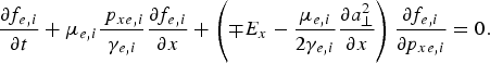
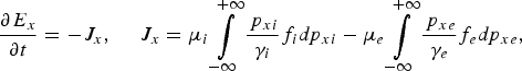
Time t is normalized to the inverse electron plasma frequency ωpe−1, length is normalized to l 0 = cωpe−1, velocity and momentum are normalized, respectively, to the velocity of light c and to M ec. In our normalized units, μe = 1 for the electrons, and μi = M e/M i = 1/1836 for the hydrogen ions. The upper sign in Eq. (1) is for electrons and the lower sign for ions. E x is calculated from Ampère's equation:
and
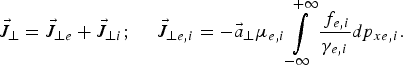
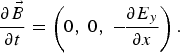
The transverse electromagnetic fields E y, B z and E z, B y for the circularly polarized wave obey Maxwell's equations. With E ± = E y ± B z and F ± = E z ± B y, we write these equations in the following form:
which are integrated along their vacuum characteristic x = t. In our normalized units, we have the following expressions for the normal current densities:
The canonical momentum ![]() is connected to the particle momentum
is connected to the particle momentum ![]() by the relation
by the relation ![]() , and
, and ![]() is the normalized vector potential.
is the normalized vector potential.
Choosing the Coulomb gauge (![]() ), we have for our 1D problem ∂a x/∂x = 0, hence a x = 0. The vector potential
), we have for our 1D problem ∂a x/∂x = 0, hence a x = 0. The vector potential ![]() , and we also have
, and we also have ![]() (Shoucri et al., Reference Shoucri, Afeyan and Charbonneau-Lefort2008). We can choose this constant to be zero without loss of generality, which means that initially all particles at a given (x, t) have the same perpendicular momentum
(Shoucri et al., Reference Shoucri, Afeyan and Charbonneau-Lefort2008). We can choose this constant to be zero without loss of generality, which means that initially all particles at a given (x, t) have the same perpendicular momentum ![]() . The transverse electromagnetic fields E y, B z for the linearly polarized wave are calculated from Eq. (4), with F ± = 0 (E z = 0, B y = 0).
. The transverse electromagnetic fields E y, B z for the linearly polarized wave are calculated from Eq. (4), with F ± = 0 (E z = 0, B y = 0).
We use a method of characteristics for the numerical solution of Eq. (1), as recently discussed in Shoucri (Reference Shoucri2008a, Reference Shoucri2008b, Reference Shoucri2008c, Reference Shoucri and Simone2008d) for instance. These methods are Eulerian that use a computational mesh to discretize the equations on a fixed grid, and have been successfully applied to different important problems in plasma physics (Shoucri, Reference Shoucri2008a, Reference Shoucri2008b, Reference Shoucri2008c, Reference Shoucri and Simone2008d), and most recently to study ion acceleration in the interaction of a high intensity circularly polarized laser wave with a plasma (Shoucri et al., Reference Shoucri2008).
3. A CIRCULARLY POLARIZED LASER BEAM INCIDENT ON AN OVERDENSE PLASMA (n/n cr = 100): ION ACCELERATION
The forward propagating circularly polarized laser wave enters the system at the left hand (x = 0) boundary, where the forward propagating fields are E + = 2E 0P r(t)cos(ωt) (E 0 is in units of M eωpec/e, time is in units of ωpe−1 and distance in units of c/ωpe), and F − = −2E 0P r(t)sin(ωt). The shape factor P r(t) = sin(πt/(2τ)) for t < τ = 50, P r(t) = 1 otherwise. A characteristic parameter of a high power laser beam is the normalized vectror potential or quiver momentum ![]() , where
, where ![]() is the vector potential of the wave. We choose for the amplitude of the potential vector
is the vector potential of the wave. We choose for the amplitude of the potential vector ![]() . For the circularly polarized wave 2a 02 = Iλ02/1.368 × 1018, I is the intensity in W/cm2, λ0 is the laser wavelength in microns. ω = 0.1ωpe, which corresponds to n/n cr = 100, where n cr is the critical density. The Lorentz factor for the transverse oscillation of an electron in the field of the wave is
. For the circularly polarized wave 2a 02 = Iλ02/1.368 × 1018, I is the intensity in W/cm2, λ0 is the laser wavelength in microns. ω = 0.1ωpe, which corresponds to n/n cr = 100, where n cr is the critical density. The Lorentz factor for the transverse oscillation of an electron in the field of the wave is ![]() . The initial distribution functions for electrons and ions are Maxwellian with temperature T e = 1 keV for the electrons and for the ions T i = 0.1 keV. We use a fine resolution in the phase-space, with N = 9000 grid points in space and 2200 grid points in momentum space for the electrons and the ions (extrema of the electron momentum are ±5, and for the ion momentum ±135.7, momentum is in units of M ec). This fine resolution of the phase-space guaranties accurate results. We use a time-step and a grid size such that Δt = Δx = 0.01885. The initial configuration is presented in Figure 1a. We have a vacuum region of length L vac 73.986 on each side of the plasma. The steep jump in density at the plasma edge on each side of the flat top density is L edge = 2.8275. In free space, ω = k for the electromagnetic wave, and λ0 = 2π/k = 62.83. It follows that λ0 ≫ L edge. The length of the central plasma slab with flat top density of 1 is L p = 16.042, so the total length of the system is L = 169.66 (in units of c/ωpe), or L = 2.7λ0. If in our units xωpe/c = a, then in the laser wave units xω/c = aω/ωpe = 0.1a. Also if tωpe = b, then tω = bω/ωpe = 0.1b. So changing the normalization to the laser wave units requires simply multiplying the time or length scales by the factor of 0.1.
. The initial distribution functions for electrons and ions are Maxwellian with temperature T e = 1 keV for the electrons and for the ions T i = 0.1 keV. We use a fine resolution in the phase-space, with N = 9000 grid points in space and 2200 grid points in momentum space for the electrons and the ions (extrema of the electron momentum are ±5, and for the ion momentum ±135.7, momentum is in units of M ec). This fine resolution of the phase-space guaranties accurate results. We use a time-step and a grid size such that Δt = Δx = 0.01885. The initial configuration is presented in Figure 1a. We have a vacuum region of length L vac 73.986 on each side of the plasma. The steep jump in density at the plasma edge on each side of the flat top density is L edge = 2.8275. In free space, ω = k for the electromagnetic wave, and λ0 = 2π/k = 62.83. It follows that λ0 ≫ L edge. The length of the central plasma slab with flat top density of 1 is L p = 16.042, so the total length of the system is L = 169.66 (in units of c/ωpe), or L = 2.7λ0. If in our units xωpe/c = a, then in the laser wave units xω/c = aω/ωpe = 0.1a. Also if tωpe = b, then tω = bω/ωpe = 0.1b. So changing the normalization to the laser wave units requires simply multiplying the time or length scales by the factor of 0.1.

Fig. 1. (a) Electron (full curve) and ion (dash curve) density profiles at tωpe = 0. (b) Electron (full curve) and ion (dash curve) density profiles at tωpe = 113.1. (c) Electron (full curve) and ion (dash curve) density profiles at tωpe = 150.8. (d) Electron (full curve) and ion (dash curve) density profiles at tωpe = 160.22. (e) Electron (full curve) and ion (dash curve) density profiles at tωpe = 320.45. (f) Electron (full curve) and ion (dash curve) density profiles at tωpe = 450. (g) Electron (full curve) and ion (dash curve) density profiles at tωpe = 650.
Figure 1 shows the plot of the density profiles against distance (full curves for the electrons and dash curves for the ions), initial profiles in Figure 1a, and then at times t = 113.1, 150.8, 160.22, 320.45, 450, and 650 (in units of ωpe−1). In Figure 1b, electrons are accelerated at the wave-front plasma-edge interface and form a density spike with a steep profile. An electric field is formed at the edge (Fig. 2b at t = 113.1), which accelerates the ions, as shown in Figure 1c. From Figure 1c and Figure 1d there is a very rapid acceleration of the ions, and a rapid build-up of an ion solitary-like structure in the ion density profile. This rapid acceleration of the ions under the combined effect of the edge electric field and the ponderomotive pressure is shown in more details in Figure 5, where the ion density peak at the wave-front plasma-edge interface jumps from a value of about 1.5 (curve a at t = 131.95) to a value of 17.5 (curve d at t = 160.22). The solitary-like structure is generated over a period of time of about 28. In the subsequent evolution in Figures 1e to 1g, we see the ions expanding to the right, forming a shock-like structure at the right boundary in Figure 1e, and then two shock-like structures in Figures 1f and 1g. This is shown in more details in Figure 2a, which presents the same density plots at times (follow the peaks from left to right) t = 113.1, 160.22, 245.05, 320.45, and 395.85, concentrating on the plasma slab region. Note in Figure 2a in the first curve at t = 113.1, the electrons (full curve) move first, while the density profile for the ions (dash curve) did not move much. The curves in Figure 1c at t = 150.8 show the ion peak reaching the electron peak at the wave-front plasma-edge interface. Then in the subsequent evolution, the ion density peak (dash curve) increases substantially and reaches a much higher value than the electron density peak at the wave-front plasma-edge interface, as indicated in Figure 1d and Figure 5 where the ion density peak reaches a value of 17.5. At the wave-front the plasma forms a steep structure, with a solitary like structure for the ions, maintaining a stable profile as the edge moves forward, as shown in Figure 2a. To the right of this edge, the accelerated high velocity ion population is now free streaming toward the right (see the ion phase-space in Fig. 6 below). The density of the ion population in this free streaming region is exactly compensated by the electron density, giving essentially no electric field in this expansion region (Fig. 2 and Fig. 3). We see in the structure in Figures 1, 2, and 4 the high solitary-like left peak at the wave-front plasma-edge interface, which propagates at a lower speed than the right smaller peak in front of the bunch of the expanding neutral plasma. The shape of a small shock-like structure with a steepening process at the right edge of the expanding ions is taking place. In Figure 2a, the high solitary-like peaks at t = 320.45 and t = 395.85 have to their immediate right two smaller ion peaks in the region of the expanding ion population. At t = 395.85, the edge at the right of the free expansion region has reached the initial plasma slab edge location and is now free streaming in the vacuum region. This is shown in more details in Figure 4, and in Figure 3a, we show the profiles at t = 450, 550, and 650 (to which we have added from Fig. 3b the corresponding electric field profiles, dash-dot curves) when the free expanding region at the right has gone beyond the initial position of the plasma edge, which was located around x ≈ 95. Figure 4 repeats the curve at t = 650 from Figure 3a. Note how the intermediate peak in the free expansion region has become important in Figures 3a and 4. The high ion solitary-like peak at the wave-front plasma-edge interface is located essentially at the same position as the electron peak in Figure 3a, with a very slight shift with respect to the electron peak. The neutrality of the free expanding region is nicely conserved, with the electron density very nicely compensating the ion density profile, resulting in essentially zero electric field in the free expansion region. In Figures 1f, 1g, 3a, and 4, a very small density ion population (dash curve) is moving backward to the left of the sharp edge discontinuity (which is not the case for the electrons who show a sharp edge at the wave front), forming small spikes. Finally, we note in Figure 4 the two shock-like structures to the right of the solitary structure at the wave-front plasma-edge interface, while in Shoucri et al. (Reference Shoucri, Afeyan and Charbonneau-Lefort2008) only one shock-like structure can be clearly seen. This multiple shoch-like structures may be due to the higher laser intensity we use in the present simulation. This point needs further investigation.

Fig. 2. (a) Plot of the density at the plasma slab (full curve electrons, dash curve ions) at (from left to right): tωpe = 113.1, tωpe = 160.22, tωpe = 245.05, tωpe = 320.45, tωpe = 395.85. (b) Electric field at (from left to right): tωpe = 113.1 (full curve), tωpe = 160.22 (dotted curve), tωpe = 245.05 (dash curve), tωpe = 320.45 (dash-dot curve), tωpe = 395.85 (dash-3dots curve).

Fig. 3. (a) Plot of the density (full curve electrons, dash curve ions) at (from left to right): (a) tωpe = 450; (b) tωpe = 550; (c) tωpe = 650 (the dash-dot curve is the corresponding electric field from Figure 3b. (b) Electric field at (from left to right): tωpe = 450 (full curve), tωpe = 550 (dash curve), tωpe = 650 (dash-dot curve).

Fig. 4. Plot of the density (full curve electrons, dash curve ions) at tωpe = 650. The dash-dot curve gives the electric field at the same time.

Fig. 5. Density profiles at the plasma edge (full curve electrons, dash curve ions) at: (a) tωpe = 131.95, (b) tωpe = 141.37, (c) tωpe = 150.8, (d) tωpe = 160.22, showing the rapid build-up of the ion density peak over a short time (the peak of the curve d) is at 17.5).

Fig. 6. (Color online) (a) Phase-space plot of the ion distribution function at tωpe = 160.22. (b) Phase-space plot of the ion distribution function at tωpe = 216.77. (c) Phase-space plot of the ion distribution function at tωpe = 320.45. (d) Phase-space plot of the ion distribution function at tωpe = 450. (e) Phase-space plot of the ion distribution function at tωpe = 650.
The electric field is presented in Figure 2b at times t = 113.1 (full curve), 160.22 (dotted curve), 245.05 (dash curve), 320.45 (dash-dot curve), and 395.85 (dash-3dots curve), and in Figure 3b at t = 450, 550, and 650 (corresponding to the density profiles in Fig. 2a and Fig. 3a, respectively). The electric field is essentially zero in the free expansion region to the right of the plasma where the free-streaming plasma is essentially neutral. Note the stable structure of the electric field peak at the wave-front plasma-edge interface, followed by a rapid decay of the electric field inside the plasma. The penetration of the electric field in the plasma is of the order of c/ωpe, as we can verify from Figures 2 to 4.
Outside the plasma in the backward direction, the electric field profiles in Figure 2b shows at t = 113.1 and t = 160.22 a shape decaying to zero away from the plasma. At t = 245.05 and at higher times in Figures 2b and 3b, the electric field shows a negative value, accelerating the small ion population in front of the edge in the negative direction. However, in Figure 4 for instance, there are only ions in the backward direction in front of the edge position at about x ≈ 95, the electrons are pushed in the forward direction by the radiation pressure of the laser pulse. The electric field is monotonic in the immediate vicinity of the plasma, but then changes sign. From Gauss Law, the derivative of the electric field is proportional to the charge density that is positive everywhere in the backward direction in front of the position x ≈ 95. However, from Figures 1e and 1f we note that the ion density in this backward direction is very small, and Figures 6c and 6b show the small density ion population moving in the backward direction sparsely populating the phase-space in this direction. We are calculating the longitudinal electric field using Ampère's law in Eq. (2). This necessitates calculating the longitudinal current by integrating as indicated in Eq. (2). In the sparsely populated low density region (Figs. 6c and 6d) in the backward direction in front of x ≈ 95, this integration is not very accurate and can result in some fluctuations in the calculated current, especially down the steep edge in front of the position x ≈ 95, where the cubic spline interpolation used in the code may result in some small negative fluctuations of the distribution function in the low density region, as it is well known when interpolating using a cubic spline along a steep gradient. So, although in Figure 2b the profiles of the electric field at t = 160.22 and t = 245.05 show the correct profiles, the steepening of the edge profile at higher times and the sparse distribution of the low density in phase-space in front of x ≈ 95 result in the calculation of the electric field in the backward direction, using Ampère's law, being flawed, building up this negative electric field as the simulation progresses. However, this low density region for x < 95 is completely decoupled from the solution propagating in the forward direction, which is our main interest. This solution propagating in the forward direction is verifying with accuracy the relations presented in Eqs. (6)–(8) (this has been verified for several values of a 0 and n/n c), and the results presented in Figure 6 in the forward direction agrees with what is presented in Figure 4 in Klimo et al. (Reference Klimo, Psikal, Limpouch and Tikhonchuk2008) and in Figure 1 of Macchi et al. (Reference Macchi, Cattani, Liseykina and Cornolti2005).
Figure 6 presents the phase-space contour plots for the ion distribution function at times t = 160.22, 216.77, 320.45, 450, and 650. The free streaming ions in Figures 6b to 6e appears on the top forming a loop, escaping the front edge region in the forward direction. The loops are very close to what has been presented in Figure 4 of Klimo et al. (Reference Klimo, Psikal, Limpouch and Tikhonchuk2008) using PIC codes. See also the recent results in Macchi et al. (Reference Macchi, Cattani, Liseykina and Cornolti2005) and Robinson et al. (Reference Robinson, Zepf, Kar, Evans and Bellei2008). Note that in Figures 6d and 6e the accelerated ions are reaching the same critical velocity after which they go to the free-streaming phase. In the backward direction, as we previously discussed, the low density sparse distribution of the ions in the phase-space in the backward direction will result in a value of the longitudinal current to be inaccurate, and consequently the value of the electric field in the backward direction calculated from Ampére's law in Eq. (2) to be inaccurate. But this region of the phase-space is completely decoupled from the forward propagating region which is our main interest, and so far did not affect its evolution. Figure 7 presents the phase-space contour plots of the electron distribution function. The steep edge at the left is due to the effect of the ponderomotive pressure pushing the electrons. Note the sharp profile at the wave-front plasma-edge interface, and the electronic population being ejected forward. We see in Figures 7c to 7f another sharp edge appearing at the right of the expansion region, as we previously mentioned in the discussion of Figure 3. At t = 450, the right edge of the free streaming expanding ions has reached the position around x = 95 (Figs. 6d and 7e), which is the original position of the plasma slab right edge (Figs.1a–1c), and at t = 650 the entire plasma has expanded beyond the position x = 95 to the right. The shape of the initial plasma slab with a plateau and sharp edges on each side is now completely modified, and replaced by a structure of a stable configuration from a bunch traveling in space with shock's structures to the left and to the right. This bunch is neutral, with the exception of the boundary at the wave-front plasma-edge interface where a steep electric field shows a penetration in the plasma on the order of c/ωpe. Figure 8 presents a closer look at the results in Figure 7f at t = 650, from x = 92 to 96, from x = 96 to 107, and from x = 107 to 113. Figure 9 presents the distribution function F e(x, p xe) at cut-offs effected in Figure 8 at x = 93.3, 95 and 102. Note a structure more or less close to symmetry in Figures 7, 8, and 9, located around p xe ≈ 0.04, since the whole structure is moving to the right.

Fig. 7. (Color online) (a) Phase-space plot of the electron distribution function at tωpe = 113.1. (b) Phase-space plot of the electron distribution function at tωpe = 160.22. (c) Phase-space plot of the electron distribution function at tωpe = 216.77. (d) Phase-space plot of the electron distribution function at tωpe = 320.45. (e) Phase-space plot of the electron distribution function at tωpe = 450. (f) Phase-space plot of the electron distribution function at tωpe = 650.

Fig. 8. (Color online) Same as Figure 7f at tωpe = 650, concentrating on the plasma region.

Fig. 9. Distribution function, obtained at cuts in the results in Figure 8 at the positions (from right to left) x ≈ 93.3, x ≈ 95. and x ≈ 102.
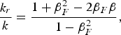
The wave-front plasma-edge interface and the solitary-like structure of the ions at the left moves at a very constant speed of 0.032 (calculated by following the left edge in Fig. 2 or Fig. 3). The velocity of the pushing front calculated in Denavit (Reference Denavit1992) by balancing the electromagnetic pressure at the absorber surface with the rate of increase in ion momentum, yields the following expression for the velocity of the surface of discontinuity:
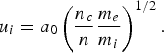
With ![]() , n/n c = 100, and m e/m i = 1/1836, we calculate u i = 0.033 (normalized to the velocity of light), in very close agreement with the measured result of 0.032 previously mentioned. At the right boundary we have neutral plasma with a smaller peak and with a shock-like structure expanding at a speed of 0.064 (can be calculated from Figs. 1–3). Between these two peaks, a neutral plasma bunch exists (with the exception of the wave-front plasma-edge interface where the penetration of the electric field is on the order of c/ωpe). This entire structure is stable as it propagates and expands to the right. The value of 0.064 for the speed of the expanding peak at the right can be recovered from Figures 6c–6e, where the momentum of the free streaming ions at the top can be estimated at M iυi/M ec ≈ 120, from which we get the velocity of the free expanding ions at right υi/c ≈ 0.0653, in very good agreement with what we calculated from Figures 1–3.
, n/n c = 100, and m e/m i = 1/1836, we calculate u i = 0.033 (normalized to the velocity of light), in very close agreement with the measured result of 0.032 previously mentioned. At the right boundary we have neutral plasma with a smaller peak and with a shock-like structure expanding at a speed of 0.064 (can be calculated from Figs. 1–3). Between these two peaks, a neutral plasma bunch exists (with the exception of the wave-front plasma-edge interface where the penetration of the electric field is on the order of c/ωpe). This entire structure is stable as it propagates and expands to the right. The value of 0.064 for the speed of the expanding peak at the right can be recovered from Figures 6c–6e, where the momentum of the free streaming ions at the top can be estimated at M iυi/M ec ≈ 120, from which we get the velocity of the free expanding ions at right υi/c ≈ 0.0653, in very good agreement with what we calculated from Figures 1–3.
Figures 10a and 11a presents the forward propagating wave E + (full curve) and the backward reflected wave E − (dash curve) at t = 254.47 and t = 320.45, respectively. Figures 10b and11b presents the corresponding results for the forward propagating wave F − (full curve) and the backward propagating wave F + (dash-curve). The electromagnetic wave damps in the plasma over a distance on the order of the skin depth c/ωpe. The strong increase of the ion and electron densities at the wave-front makes the plasma more opaque, with the steep plasma edge acting as a moving mirror for the incident light. Note that when E + is maximum, F − is minimum, and vice-versa, so the wave is always maintaining a pressure on the surface of the plasma. The frequency of the backward reflected wave is slightly down-shifted by the moving reflecting plasma surface, which is acting as a mirror. Note in Figure 10a at t = 254.475, when the incident and reflected waves are in phase at the reclection point, the reflected wave (dash curve) in vacuum has a wavelength (and a period) slightly bigger than the corresponding ones for the incident wave (full curve). Hence, the frequency of the reflected wave is slightly down-shifted with respect to the frequency of the incident wave by the Doppler shift due to the motion of the moving plasma surface, acting as a mirror. In Guérin et al. (Reference Guérin, Mora, Adam, Héron and Laval1996), the following analytical expressions were derived for the reflected wave number k r and the reflected frequency ωr of the laser wave due to the Doppler shift by the moving reflecting surface:
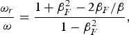
where in our units βF = u i = 0.032 is the normalized velocity of the discontinuity surface from Eq. (6), and β = ω/k = 1 for the incident wave, since ω = k = 0.1 for the incident laser wave in free space. We get for the reflected wave in free space from Eqs. (7) and (8) ωr/ω = k r/k = 0.938. This is confirmed if we follow the peaks of the reflected wave in Figures 10 and 11 (dash-curve). We find a wavelength for the reflected wave of 66.698, which corresponds to k r = 0.0942, in close agreement to what is calculated from Eq. (8). Figure 12 shows the frequency spectrum of the incident wave (full curve) and of the reflected wave (dash-curve), monitored close to the entrance of the domain at x = 0.9. The incident wave has a frequency of 0.1 as it should. The small down-shift in the frequency of the reflected wave is confirmed. However, it cannot be quantified since in our frequency spectrum, we have dω = 0.0203. With ωr = 0.0938 calculated from Eq. (7), this corresponds to a shift with respect to ω = 0.1 of only 0.0062, below the resolution of our frequency spectrum. However, we can confirm the value of the frequency down-shift if we follow the period of the oscillation of the reflected signal at x = 0.9.

Fig. 10. (a) Incident wave E +(full curve) and reflected wave E −(dash curve) at tωpe = 254.47. (b) Incident wave F − (full curve) and reflected wave F + (dash curve) at tωpe = 254.47.
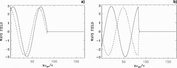
Fig. 11. (a) Incident wave E +(full curve) and reflected wave E − (dash curve) at tωpe = 320.45. (b) Incident wave F − (full curve) and reflected wave F + (dash curve) at tωpe = 320.45.

Fig. 12. Frequency spectrum of the incident wave E +(full curve) and reflected wave E − (dash curve) monitored close to the entrance of the domain at x ≈ 0.94 (the frequency is normalized to the plasma frequency ωpe).
4. A LINEARLY POLARIZED LASER BEAM INCIDENT ON AN OVERDENSE PLASMA (n/n cr = 100): HARMONICS GENERATION
The forward propagating linearly polarized laser wave enters the system at the left-hand (x = 0) boundary, where the forward propagating field is E + = 2E 0P r(t)cos(ωt) and F − = 0 (E 0 is in units of M eωpec/e, time is in units of ωpe−1, and distance in units of c/ωpe) . The shape factor P r(t) = sin(πt/(2τ)) for t < τ = 50, and P r(t) = 1 otherwise. We choose for the amplitude of the potential vector ![]() . For the linearly polarized wave a 02 = Iλ02/1.368 × 1018, I is the intensity in W/cm2, λ0 is the laser wavelength in microns. ω = 0.1ωpe, which corresponds to n/n cr = 100, where n cr is the critical density. The Lorentz factor for the transverse oscillation of an electron in the field of the wave is
. For the linearly polarized wave a 02 = Iλ02/1.368 × 1018, I is the intensity in W/cm2, λ0 is the laser wavelength in microns. ω = 0.1ωpe, which corresponds to n/n cr = 100, where n cr is the critical density. The Lorentz factor for the transverse oscillation of an electron in the field of the wave is ![]() . The initial distribution functions for electrons and ions are Maxwellian with temperature T e = 1 keV for the electrons and for the ions T i = 0.1 keV. We use a fine resolution in phase-space, with N = 10000 grid points in space and 2000 grid points in momentum space for the electrons and the ions, respectively (extrema of the electron momentum are ±5, and for the ion momentum ±122.88, momentum is in units of M ec). We use a time-step and a grid size such that Δt = Δx = 0.01885. We have adjusted the number of grid points in space N to keep the same Δx and Δt as in the case presented in Section 3. We have a vacuum region of length L vac = 73.986 on each side of the plasma, and the steep jump in density at the plasma edge on each side of the flat-top density is L edge = 2.8275, as in Section 3. In free space ω = k for the electromagnetic wave, and λ0 = 2π/k = 62.8. It follows that λ0 ≫ L edge. The length of the central plasma slab with flat-top density of 1 is L p = 34.89, longer in this case than in Section 3, which is necessary for a good study of the interaction in the present problem. The total length of the system is L = 188.5 (in units of c/ωpe). In this case, we have L = 3λ0.
. The initial distribution functions for electrons and ions are Maxwellian with temperature T e = 1 keV for the electrons and for the ions T i = 0.1 keV. We use a fine resolution in phase-space, with N = 10000 grid points in space and 2000 grid points in momentum space for the electrons and the ions, respectively (extrema of the electron momentum are ±5, and for the ion momentum ±122.88, momentum is in units of M ec). We use a time-step and a grid size such that Δt = Δx = 0.01885. We have adjusted the number of grid points in space N to keep the same Δx and Δt as in the case presented in Section 3. We have a vacuum region of length L vac = 73.986 on each side of the plasma, and the steep jump in density at the plasma edge on each side of the flat-top density is L edge = 2.8275, as in Section 3. In free space ω = k for the electromagnetic wave, and λ0 = 2π/k = 62.8. It follows that λ0 ≫ L edge. The length of the central plasma slab with flat-top density of 1 is L p = 34.89, longer in this case than in Section 3, which is necessary for a good study of the interaction in the present problem. The total length of the system is L = 188.5 (in units of c/ωpe). In this case, we have L = 3λ0.
There are substantial differences in several aspects when circular or linear polarization for the incident laser wave is considered. We analyze first the linear response. If we assume a linearly polarized wave: ![]() , we can write a linear analysis E y = E 0 cos (ψ), ψ = (kx − ωt). Faraday's law is:
, we can write a linear analysis E y = E 0 cos (ψ), ψ = (kx − ωt). Faraday's law is:
Then ![]() with B z = B 0 cos (ψ), and B 0 = E 0 k/ω. From
with B z = B 0 cos (ψ), and B 0 = E 0 k/ω. From ![]() and
and ![]() , we get
, we get ![]() with p y = −p 0 sin (ψ), and p 0 = E 0/ω. The longitudinal Lorentz force is p yB z = −1/2 kp 02 sin (2ψ). This drives a longitudinal response at the second harmonic of the laser wave. In a circular polarization, we have for the laser wave in a linear analysis
with p y = −p 0 sin (ψ), and p 0 = E 0/ω. The longitudinal Lorentz force is p yB z = −1/2 kp 02 sin (2ψ). This drives a longitudinal response at the second harmonic of the laser wave. In a circular polarization, we have for the laser wave in a linear analysis ![]() . From Faraday's law:
. From Faraday's law:
Which gives ![]() and
and ![]()
![]() . Thus, we see that
. Thus, we see that ![]() is identically zero,
is identically zero, ![]() and
and ![]() are parallel. So in the case of a circular polarization there is no second harmonic longitudinal response to the leading order.
are parallel. So in the case of a circular polarization there is no second harmonic longitudinal response to the leading order.
Figure 13 shows the plot of the density profiles against distance (full curves for the electrons and dash curves for the ions) at times t = 113.1, 169.65, 188.5, and 450. At t = 113.1 there is a build-up of the electron density at the left edge in front of the incident wave. Initially, electrons move first under the influence of the ponderomotive pressure forming a steep edge (Fig. 14a). The position of this electron density steep edge remains essentially around x ≈ 79 during the simulation, and does not propagate, but rather shows an oscillation around x ≈ 79. Figures 13b and 13c at times t = 169.65 and 188.5, respectively, show the rapid build-up of a solitary-like structure for the ion density peak, similar to what we have seen in Section 3. The oscillation of the edge at the harmonic of the wave frequency under the effect of the ponderomotive pressure will be discussed in more details in Figure 14, where we concentrate the plots on the wave-front plasma-edge region. Note also an important oscilation in the density profiles due to the electrons being pushed forward by the wave.

Fig. 13. (a) Electron (full curve) and ion (dash curve) density profiles at tωpe = 113.1. (b) Electron (full curve) and ion (dash curve) density profiles at tωpe = 169.65. (c) Electron (full curve) and ion (dash curve) density profiles at tωpe = 188.5. (d) Electron (full curve) and ion (dash curve) density profiles at tωpe = 450.
The associated electric fields due to the charge separation are given by the dash-dot curves in Figure 14. Figure 14a is showing a steep edge of the electron density at the wave-front plasma-edge interface (full curve), and the formation of a relatively thin ion solitary peak, which is growing and reaching its maximum in Figure 14b at t = 188.5. In Figure 14b, the electron density at the wave-front is not steep anymore, but is rather decaying slowly from x ≈ 78 to x ≈ 75. An explanation can be found in Figure 16a, which shows the incident wave E +(full curve), and the reflected wave E − (dash curve), at time t = 188.5. The incident wave E + is about zero at the edge, i.e., there is no radiation pressure exerted by the wave on the plasma surface around time t = 188.5, which explains the slow decay of the electron density profile at the edge. Then the amplitude of the incident wave starts rising again at the wave-front plasma-edge interface, and at t = 197.92 in Figure 14c we see a steep electron density at the edge. At the same time in Figure 16b we are close to a peak of the incident wave at the edge, or sufficiently close to the peak for the wave to be intense enough to exert a pressure that steepens the electron density edge. As we have discussed above for the linear response in the case of a linear polarization, the period of oscillation of the electron edge, at the harmonic frequency of the incident wave, is 31.4. The difference in time between Figures 14b and 14c (or between Figs. 16a and 16b) is 9.42, close to the quarter period of the edge oscillation of 31.4/4 ≈ 8. At t = 235.62 in Figure 14d, we have a steep electron density profile at the edge, corresponding to a peak in the incident wave field E +at the same time in Figure 16c. Figure 14e at t = 414.7 is showing the motion of the edge at a time in the oscillation cycle where the edge electrons are being pushed back to the right in the forward direction by the incident wave, showing at t = 424.12 in Figure 14f and at t = 433.55 in Figure 14g, the formation of a steeper edge. The oscillation of the edge electron density profile is not uniform. We see in Figure 14h at t = 442.97 the edge electrons expanding rapidly to the left, and then pushed to the right again in Figure 14i, to repeat the cycle that started in Figure 14e. In the selection we have for the plots, the time spent between Figures 14e and 14i is 35.3, close to the period of the oscillation of the ponderomotive force at twice the laser frequency, which is 31.4. The edge of the electrons in Figure 14g at t = 433.55 is around x ≈ 80. Figure 16d presents the incident wave E + (full curve) and the reflected wave E − (broken curve) at t = 433.55, at the time where the electrons are moving to form a steep edge at the left boundary (see Fig. 14g). Indeed, in Figure 16d the incident wave is finite at the edge, and exerts a pressure on the electron density profile. The wave did not reach its peak yet, but is sufficiently strong to push the edge electrons, who in Figure 14g are on their way to form again a steep edge. Due to the build-up of the plasma density at the edge, which makes the plasma more opaque, the wave is strongly damped at the edge and consequently the wave penetration is small. At t = 442.97 in Figure 14h the edge expands to the left reaching a position around x ≈ 75. Figure 16e shows the corresponding E + and E − profiles at the same time t = 442.97, and we note the incident wave is about zero at the edge, and exerts negligible pressure on the electron density profile, which is then expanding to the left as in Figure 14h.

Fig. 14. (a) Electron (full curve) and ion (dash curve) density profiles, and electric field (dash-dot curve) at tωpe = 169.65. (b) Electron (full curve) and ion (dash curve) density profiles, and electric field (dash-dot curve) at tωpe = 188.5. (c) Electron (full curve) and ion (dash curve) density profiles, and electric field (dash-dot curve) at tωpe = 197.92. (d) Electron (full curve) and ion (dash curve) density profiles, and electric field (dash-dot curve) at tωpe = 235.62. (e) Electron (full curve) and ion (dash curve) density profiles, and electric field (dash-dot curve) at tωpe = 414.7. (f) Electron (full curve) and ion (dash curve) density profiles, and electric field (dash-dot curve) at tωpe = 424.12. (g) Electron (full curve) and ion (dash curve) density profiles, and electric field (dash-dot curve) at tωpe = 433.55. (h) Electron (full curve) and ion (dash curve) density profiles, and electric field (dash-dot curve) at tωpe = 442.97. (i) Electron (full curve) and ion (dash curve) density profiles, and electric field (dash-dot curve) at tωpe = 450.
An average velocity of the edge between Figures 14g and 14h is approximately (80–75)/(442.97–433.55) = 0.53 (normalized to the velocity of light), which is substantial. During this rapid oscillation of the electron density edge, the steep ion density edge in Figure 14 (broken curves) at x ≈ 81 shows a little local peak and seems to vary very little, drifting slowly to the right. The ion density thin solitary-like peak on the other hand seems to propagate slowly to the right in the forward direction, between x ≈ 85.2 at t = 414.7 in Figure 14e, to x ≈ 86.1 at t = 450 in Figure 14i. We plot the edge electric field at times t = 414.7 (full curve), 433.55 (broken curve), and 450 (dash-dot curve) in Figure 15, which shows in the region of the plasma edge the same period of oscillation as for the ponderomotive force. The electric field at the plasma edge is following the oscillation of the edge electrons. The high peak in Figure 15 at t = 433.55 corresponds to the steep edge in Figure 14g (see the dash-dot curve in Fig. 14g for the electric field). This oscillation contrasts with the steady profiles of the electric field at the edge obtained in Figure 3 for the case of a circular polarization. In addition, we see in Figure 15 around x ≈ 86. a stable steady-state profile of the electric field showing a steep rapid variation in space from a negative to positive value, which will be discussed in Figure 18 below, for the ion phase-space.

Fig. 15. Electric field profiles at tωpe = 414.7 (full curve), tωpe = 433.55 (dash curve), and tωpe = 450 (dash-dot curve).
The results in Figure 16 showing the incident wave at the plasma surface going through maxima and zero vlalues contrast with what we see in Figures 10–12 and also explain the results obtained in Section 3, where for a circularly polarized wave, when the incident wave E + is minimum at the edge, the other incident wave F − is maximum, and vice-versa. So there is always an incident wave exerting pressure on the electron density profile at the edge in the case of a circular polarization, which causes this edge to remain steep and to move always in the forward direction, as observed in the results in Section 3.

Fig. 16. (a) Incident wave E +(full curve) and reflected wave E − (dash curve) at tωpe = 188.5. (b) Incident wave E +(full curve) and reflected wave E − (dash curve) at tωpe = 197.92. (c) Incident wave E +(full curve) and reflected wave E − (dash curve) at tωpe = 235.62. (d) Incident wave E +(full curve) and reflected wave E − (dash curve) at tωpe = 433.55. (e) Incident wave E +(full curve) and reflected wave E − (dash curve) at tωpe = 442.97.
The relativistic oscillation of the electron density surface in the field of the high intensity wave is nonlinear, and can thus generate harmonics (similar to the relativistic oscillating mirror, see Baeva et al. (Reference Baeva, Gordienko and Pukhov2006)). The signature of the harmonics in the distorted shape of the reflected wave (dash curve) is obvious in Figure 16. Figure 17 shows the frequency spectrum of the incident signal with a peak at ω = 0.1 (full curve, with a peak of 200), and the frequency spectrum of the reflected signal with peaks at ω = 0.1, and 3ω, 5ω, 7ω, 9ω … (broken curve, the peak at ω = 0.1 is reaching 130). The presence of odd harmonics in the reflected signal, at normal incidence of the laser wave, is due to relativistic effects as has been discussed in several publications (Bulanov et al., Reference Bulanov, Naumova and Pegoraro1994; Lichters et al., Reference Lichters, ter Vehn and Pukhov1996; Wilks et al., Reference Wilks, Kruer and Mori1993, also see Teubner & Gibbon, Reference Teubner and Gibbon2009).

Fig. 17. Frequency spectrum of the incident wave E +(full curve) and reflected wave E − (dash curve) monitored close to the entrance of the domain at x ≈ 0.94 (the frequency is normalized to the plasma frequency ωpe).
Figure 18 shows the phase-space plots of the ion distribution function. Figure 18a at t = 188.5 shows the acceleration of the ions at the edge. Figure 18b at t = 235.62 shows the appearance of an X-like structure on the vertical line, showing a pattern of bifurcation in the phase-space. Figure 18c shows the phase-space at t = 450. Figure 19 repeats Figure 18b, concentrating on the X-like structure. This structure at x ≈ 81 in Figure 19 corresponds to the position of the high ion solitary peak in Figure 14d. At this position, the electric field shows a steady-state profile with rapid variation in space between negative and positive values, and is therefore pushing the ions in opposite directions, resulting in the formation of the observed X structure. For instance, at t = 450, the dash-dot curve in Figure 15 shows this rapid variation from negative to positive values around x ≈ 86, corresponding to the structure in Figure 18c.

Fig. 18. (Color online) (a) Phase-space plot of the ion distribution function at tωpe = 188.5. (b) Phase-space plot of the ion distribution function at tωpe = 235.62. (c) Phase-space plot of the ion distribution function at tωpe = 450.

Fig. 19. (Color online) Same as Figure 18b at tωpe = 235.62, concentrating around x ≈ 81.
Figure 20 presents the phase-space plots of the electron distribution function at t = 188.5, 235.62, 442.97, and 450. In Figure 20a, electrons are accelerated forward, and have a steep profile at the wave-front plasma-edge interface. In Figures 20c and 20d, we see the oscialltion of the edge during the evolution of the system. The electrons at the edge are rapidly moving between negative and positive velocities, and this strong oscillation contrasts with the more stable drifting structure obtained in Figure 7 for the case of a circular polarization. In Figure 20, the electron distribution function shows a heating more important than in the results presented in Section 3. The hot electrons are accelerated forward and penetrate the plasma, as we can see from the oscillation of the electron density in the plots in Figure 13, even though the electromagnetic wave damps strongly at the edge and does not show penetration in the plasma (see Fig. 16).

Fig. 20. (Color online) (a) Phase-space plot of the electron distribution function at tωpe = 188.5. (b) Phase-space plot of the electron distribution function at tωpe = 235.62. (c) Phase-space plot of the electron distribution function at tωpe = 442.97. (d) Phase-space plot of the electron distribution function at tωpe = 450.
5. CONCLUSION
In the present paper, we have used an Eulerian-Vlasov code for the numerical solution of the 1D relativistic Vlasov-Maxwell equations to study the interactions at the surface of overdense plasma under the effect of a high intensity normally incident laser beam. Generally, the electrons are pushed by the ponderomotive pressure, forming a gradient at the wave-front plasma-edge interface. This generates a charge separation and an electric field at the plasma edge that accelerates the ions. All the results presented point to the importance of the dynamic of the ions at the wave-front plasma-edge interface in the evolution of the system. There is a phase where the ions go through a very rapid build-up of a solitary like structure of the ion density at the plasma edge. This rapid ion acceleration in laser-plasma interaction has been discussed for instance in Esirkepov et al. (Reference Esirkepov, Borghesi, Bulanov, Mourou and Tajima2004). We are far from the picture of heavy immobile ions at the plasma edge that act to prevent the expansion of the electrons.
The results obtained differ substantially in several aspects when circular or linear polarization for the incident laser wave is considered (see Macchi et al., Reference Macchi, Cattani, Liseykina and Cornolti2005; Liseykina et al., Reference Liseykina, Borghesi, Macchi and Tuveri2008). We used in the present set of simulations the condition λ0 ≫ L edge and n/n cr ≫ 1. For the case of a circular polarization, Figures 4 and 7 show a steep density gradient with a shock-like structure for the electrons at the wave-front edge, while the ion profiles in Figure 4 shows the formation of sharp solitary-like structures where the acceleration of the ions takes place. There is a very small density ion population being left behind to the left of the wave-front plasma-edge interface. The moving steep plasma edge acts as a moving mirror reflecting the incident wave. Following the acceleration phase of the ions, there is a fraction of the ions that reach a free streaming expansion state in the forward direction, with the electrons compensating the charge of the expanding ions. The loop at the top of the phase-space in Figures 6c–6e originates from the ballistic evolution of the fraction of the expanding ions that form with the electrons a neutral “bunch” with narrow energy spectrum directed in the forward direction. This planar free expansion phase of a neutral plasma bunch at the right boundary is associated also with the formation of shock-like structures and sharp ion front with ion peaks or spikes in the local ion density (called bunching), as observed in the present simulation. There is qualitative agreement between some phase-space features presented in Figures 6c–6e and recent PIC results (see Fig. 4 in Klimo et al. (Reference Klimo, Psikal, Limpouch and Tikhonchuk2008), and also some of the plots in Fig. 1 of Macchi et al. (Reference Macchi, Cattani, Liseykina and Cornolti2005)).
Laser-driven ion beams have properties that differ in several aspects from beams of comparable energy obtained from conventional acceleration techniques, and have the potential to be applied in a number of innovative applications in the scientific, technological and medical areas as mentioned in the introduction, and for ion-driven fast ignition (Fernandez et al., Reference Fernandez, Honrubia, Albright, Flippo, Gautier, Hegelich, Schmitt, Temporal and Yin2009). They also play a fundamental role in a number of physical situations where plasma jets of high speed are observed. It is believed to provide the main acceleration mechanism for cosmic rays at the front of collisionless shock waves generated during supernova explosions (Berezinskii et al., Reference Berezinskii, Bulanov, Dogiel, Ginzburg and Ptuskin1990).
We have presented in Section 4 a case of a linearly polarized wave incident on an overdense plasma under the condition λ0 ≫ L edge and n/n cr ≫ 1, with a normal incidence of the laser beam. With a set of parameters essentially close to those used in Section 3, odd harmonics have been generated in the reflected wave (Bulanov et al., Reference Bulanov, Naumova and Pegoraro1994; Lichters et al., Reference Lichters, ter Vehn and Pukhov1996; Wilks et al., Reference Wilks, Kruer and Mori1993; Teubner & Gibbon, Reference Teubner and Gibbon2009). The intense linearly polarized laser pulse interacting with a near discontinuous plasma-vacuum interface causes the electron density surface to perform relativistic oscillations with a frequency equal to twice the laser wave frequency, due to the ponderomotive force (see Figs. 14e–14c, and the linear analysis we presented at the beginning of Section 4). Figure 16 and the phase-space plots in Figures 18 and 20 show the complexity of the structures generated at the wave-front plasma-edge interface, and the strong oscillation of the electrons, especially at the interface. Recent results have shown the generation of high intensities attosecond pulses, combining short wavelengths and very high time resolution, which open applications to new fields in physics. The very recent works in Teubner and Gibbon (Reference Teubner and Gibbon2009) and Lavocat-Dubuis and Matte (Reference Lavocat-Dubuis and Matte2009) contain a nice review on the problem of harmonics generation.
ACKNOWLEDGMENTS
M. Shoucri acknowledges the constant support and encouragement of Dr. Guy Bélanger and Dr. André Besner, and is also grateful to the Centre de calcul scientifique de l'IREQ (CASIR) for computer time used to do part of this work. The work of B. Afeyan was funded by a DOE NNSA SSAA grant and by P-24 at Los Alamos National Laboratory. B. Afeyan has benefited greatly by conversations with Juan Fernandez on the matter of proton acceleration by ultraintense lasers.


