Introduction
The interactions of ion beams with plasmas are analyzed in a large quantity of fields of physics. Specifically, measurements of energy losses of these ion beams in plasmas are studied (Mintsev et al., Reference Mintsev, Gryaznov, Kulish, Filimonov, Fortov, Sharkov, Golubev, Fertman, Turtikov and Vishnevskiy1999; Zylstra et al., Reference Zylstra, Frenje, Grabowski, Li, Collins, Fitzsimmons, Glenzer, Graziani, Hansen and Hu2015). One example is the slowing down analysis of swift ions when they pass through diluted and ionized interstellar matter (Deutsch et al., Reference Deutsch, Maynard, Chabot, Gardes, Della-Negra, Bimbot, Rivet, Fleurier, Couillaud and Hoffmann2010). Another example is the production and diagnosis of warm dense matter through the energy loss of projectile ions (Casas et al., Reference Casas, Andreev, Schnuerer, Barriga-Carrasco, Morales and Gonzalez-Gallego2016). The energy losses of swift charged particles in plasmas are also deeply analyzed in fusion research, as they play a relevant role to determine the beam energy deposition inside a fuel target. The understanding of the energy deposition can open the way to energetic applications, like inertial confinement fusion, where ion beams are used to achieve the extreme density and temperature conditions that plasma needs to fusion (Deutsch, Reference Deutsch1986; Frank et al., Reference Frank, Blazević, Bagnoud, Basko, Borner, Cayzac, Kraus, Hessling, Hoffmann and Ortner2013). Then, a complete theoretical method for the stopping power of the plasma is required to estimate properly the energy deposition of projectile ions.
The stopping power of plasmas is more easy to study when plasmas are fully ionized, that is, when the plasma ions have been stripped off all their electrons. But it can be also studied for partially ionized plasmas, when the plasma ions keep some of their electrons (Barriga-Carrasco & Casas, Reference Barriga-Carrasco and Casas2013). In the last case, the electron stopping power can be divided in two parts: a first part due to free electrons and a second one coming from bound electrons.
For free electrons case, dielectric formalism can be used and many dielectric functions can be utilized, for instance the random phase approximation (RPA) which is valid in plasmas of all degeneracies (Barriga-Carrasco, Reference Barriga-Carrasco2010). In RPA, the energy transfer to a target is proportional to the square of the projectile charge and the projectile can be considered as a perturbation. The use of dielectric functions often involves the resolution of very large integrals to obtain the stopping power, which requires a great quantity of computational time. To solve this problem, an interpolation from a database of stopping powers that includes a wide range of plasma temperatures and densities is used (Barriga-Carrasco, Reference Barriga-Carrasco2013).
For bound electrons case, the atomic properties can be determined in the context of the average atom (Mayer, Reference Mayer1947) or in the detailed atom description, where all charge states of the chemical element are considered. On the other hand, the mean excitation energy (Garbet et al., Reference Garbet, Deutsch and Maynard1987), which plays an important role in our stopping power model, can be determined by oscillator strength sums (Bell et al., Reference Bell, Bish and Gill1972; Casas et al., Reference Casas, Barriga-Carrasco and Rubio2013) and Hartree–Fock claculations (Fischer, Reference Fischer1987; Haken et al., Reference Haken, Brewer and Wolf2006). In this work, detailed atom description will be used for the helium plasma, the mean excitation energy will be considered for each shell of the ion, and not for each atom as a whole, and they will be obtained from Hartree–Fock calculations.
In the Theoretical methods section, our theoretical methods for atomic kinetic and stopping power calculations and a short explanation for plasma thermodynamic states will be given. Afterwards, in the Results section, the results obtained with our theoretical models are discussed and compared with experimental data. Finally, the conclusions will be shown up in the Conclusions section. The units used in this work are atomic units (a.u.),  $e = \hbar = m_e = 1$, in equations and formulas if others are not stated. Spectroscopic notation is used for helium ions.
Theoretical methods
Stopping power
The total stopping power of partially ionized matter can be estimated through two contributions, free and bound electrons (Barriga-Carrasco & Maynard, Reference Barriga-Carrasco and Maynard2005; Barriga-Carrasco & Casas, Reference Barriga-Carrasco and Casas2013):
 $$Sp = Sp_{{\rm free}} + Sp_{{\rm bound}}$$
The free electron stopping power is estimated as
 $$Sp_{{\rm free}} = \displaystyle{{4\pi Z^2} \over {v_{\rm p}^2}} n_{{\rm at}} \times Q \times L_{{\rm fe}},$$
where Z is the constant charge (point-like without charge extension) of the projectile and v p is the velocity of the projectile, respectively. The atomic density of the plasma is n at and the mean plasma ionization is Q, resulting the free electron density, n fe = n at × Q. The stopping number of plasma-free electrons is L fe, that will be analyzed later.
The bound electron stopping power is obtained as the sum of the bound stopping of each helium species (Casas et al., Reference Casas, Barriga-Carrasco and Rubio2013, Reference Casas, Andreev, Schnuerer, Barriga-Carrasco, Morales and Gonzalez-Gallego2016) in the ground state,
 $$Sp_{{\rm bound}} = N_{{\rm HeI}} \times Sp_{{\rm boundHeI}} + N_{{\rm HeII}} \times Sp_{{\rm boundHeII}}$$
where N HeI and N HeII are the abundances of the HeI and HeII ions, respectively, and being the bound stopping power of any species,
 $$Sp_{{\rm boundS}} = \displaystyle{{4\pi Z^2} \over {v_{\rm p}^2}} n_{{\rm at}}\sum\limits_i P_iL_{{\rm be},i}$$
where L be,i and P i are the stopping number of bound electrons and the number of electrons for a i shell of the ion species in the target. The total bound electron density of the plasma is  $n_{{\rm be}} = n_{{\rm at}}(N_{{\rm HeI}} \times \sum\nolimits_i P_{{\rm HeI}i} + N_{{\rm HeII}} \times \sum\nolimits_i P_{{\rm HeII}i})$.
In Eq. (2), free electron stopping number, L fe, can be computed using the dielectric formalism, through RPA dielectric function, εRPA (Arista & Brandt, Reference Arista and Brandt1984; Maynard & Deutsch, Reference Maynard and Deutsch1985), developed in terms of the wave number k and the frequency ω provided by quantum mechanics analysis. The expression for RPA is (Lindhard, Reference Lindhard1954):
 $${\rm \epsilon} _{{\rm RPA}}(k,\omega ) = 1 + \displaystyle{1 \over {\pi ^2k^2}}\int d^3{k}^{\prime}\displaystyle{{\,f\,(\overrightarrow k + \overrightarrow {{k}^{\prime}} ) - f\,(\overrightarrow {{k}^{\prime}} )} \over {\omega + i\nu - (E_{\overrightarrow k + \overrightarrow {{k}^{\prime}}} - E_{\overrightarrow {{k}^{\prime}}} )}},$$
where  $E_{\overrightarrow {{k^{\prime}}}} = k^2/2$, and temperature dependence is shown through the Fermi–Dirac function:
 $$f\,(\overrightarrow k ) = \displaystyle{1 \over {1 + {\rm exp}[\beta (E_k - \mu )]}},$$
where β = 1/(k BT) and μ is the chemical potential of the plasma with an electron density n fe and temperature T; and k B is the Boltzmann constant. If the absence of collisions is assumed, the collision frequency ν → 0. An analytic RPA dielectric function for plasmas at any degeneracy can be obtained from Eq. (5) (Arista & Brandt, Reference Arista and Brandt1984):
 $${\rm \epsilon} _{{\rm RPA}}(k,\omega ) = 1 + \displaystyle{1 \over {4z^3\pi k_{\rm F}}}[g(u + z) - g(u - z)],$$
where u = ω/(kν F) and z = k/(2k F) are dimensionless variables (Lindhard, Reference Lindhard1954) and  $k_{\rm F} = \nu _{\rm F} = \sqrt {2E_{\rm F}} $ is the Fermi velocity. g(x) is defined as:
 $$g(x) = \int_0^\infty \displaystyle{{ydy} \over {{\rm exp}(Dy^2 - \beta \mu ) + 1}}{\rm ln}\left( {\displaystyle{{x + y} \over {x - y}}} \right),$$
where D = E Fβ is the degeneracy parameter.
Finally, the free electronic contribution can be calculated as:
 $$L_{{\rm fe}} = \displaystyle{1 \over {2\pi ^2n_{{\rm at}}Q}}\int_0^\infty \displaystyle{{dk} \over k}\int_0^{kv} \omega d\omega {\rm Im}\left[ { - \displaystyle{1 \over {{\rm \epsilon} _{{\rm RPA}}(k,\omega )}}} \right].$$
The bound electrons stopping power for any species, Sp boundS, can be determined from atomic calculations to estimate atomic properties, using the Hartree–Fock method. Using the classic Bethe formula (Bethe, Reference Bethe1930), it can be seen that it cannot fit well the stopping power when the velocity is low due to the logarithm that gives a negative value if its argument is below 1. To avoid this, the stopping number for bound electrons L be is obtained from an interpolation between high and low projectile velocity approximation (Maynard & Deutsch, Reference Maynard and Deutsch1985; Barriga-Carrasco & Maynard, Reference Barriga-Carrasco and Maynard2005):
 $$L_{{\rm be},i}(v_{\rm p}) = \left\{ {\matrix{ {L_{{\rm H},i}(v_{\rm p}) = {\rm ln}\left( {\displaystyle{{2v_{\rm p}^2} \over {I_i}}} \right) - \displaystyle{{2K_i} \over {v_{\rm p}^2}} \quad {\rm for}\,v_{\rm p} \gt v_{{\rm int},i}} \hfill \cr {L_{{\rm B},i}(v_{\rm p}) = \displaystyle{{\alpha _iv_{\rm p}^3} \over {1 + G_iv_{\rm p}^2}} \quad\quad\quad\; {\rm for}\,v_{\rm p} \le v_{{\rm int},i}} \cr}} \right.,$$
where K i is the electronic kinetic energy,  $\alpha _i = 1.067K_i^{1/2} I_i^{ - 2} $ is the hydrogenic approximation friction coefficient for low velocities, and v int,i = (3K i + 1.5I i)1/2 is an intermediate velocity that links both expressions without discontinuity. G i is obtained when L H,i(v int,i) = L B,i(v int,i). The mean excitation energy can be obtained from the following expression (Garbet et al., Reference Garbet, Deutsch and Maynard1987; Barriga-Carrasco & Maynard, Reference Barriga-Carrasco and Maynard2005):
 $$I_i = \sqrt {\displaystyle{{2K_i} \over {\langle r_i^2 \rangle}}}, $$
where  $\langle r_i^2 \rangle $ is the quadratic mean radius for an electron at the i shell. The mean excitation energy is calculated using Eq. (11) from K i and
  $\langle r_i^2 \rangle $ using the Hartree–Fock method implemented in Fortran 90 (Casas et al., Reference Casas, Andreev, Schnuerer, Barriga-Carrasco, Morales and Gonzalez-Gallego2016). This calculation method has the advantage of estimating the stopping power shell by shell, instead of considering it as a global average value.
Plasma thermodynamic states
As it is well known, for a given plasma conditions, plasma could be in local thermal equilibrium (LTE) or non-local thermal equilibrium (NLTE) themodynamics states. The average ionization and ionic abundances change with the thermodynamic states, then the thermodynamic states of the plasma influence on the calculation of its stopping power as the stopping power relies on the average ionization and ionic abundances.
LTE case happens in plasmas in which dimensions are lower than the mean free path of the photons emitted in its interior, but larger than the length traveled by electrons between consecutive collisions with an ion. For this case, atomic-level populations are given by Saha–Boltzmann equation (Saha, Reference Saha1921; Dendy, Reference Dendy1995):
 $$n_{{\rm fe}}\displaystyle{{n_{r + 1}} \over {n_r}} = \left( {\displaystyle{{U_{r + 1}} \over {U_r}}} \right)\left( {2\displaystyle{{{(2\pi k_{\rm B}T)}^{3/2}} \over {h^3}}} \right)e^{\displaystyle{{ - \chi _r} \over {Tk_{\rm B}}}},$$
 $$U_r = \sum\limits_i g_{ri}{\rm exp}( - {\rm \epsilon} _{ri}/k_{\rm B}T),$$
where n fe, n r, n r+1 are the free electron densities for the ionized atoms, r or r + 1 times ionized, respectively; U r and U r+1 are the partition functions of the ions, h is the Planck constant (h = 2π for atomic units), χ r the ionization potential, g ri is the statistical weight, and εri is the energy of the ith state.
However, for most cases, a plasma do not verify the previous conditions, so it is in NLTE case. The general method to calculate atomic abundances is based on collisional-radiative model (McWhirter, Reference McWhirter1978). The rate equations describe the abundance of the atomic states:
 $$\displaystyle{{dN_{\zeta m}(\vec r,t)} \over {dt}} = \sum\limits_{{\zeta} ^{\prime}{m}^{\prime}} N_{{\zeta} ^{\prime}{m}^{\prime}}(\vec r,t){\rm {\open R}}_{{\zeta} ^{\prime}{m}^{\prime} \to \zeta m}^ + - \sum\limits_{{\zeta} ^{\prime}{m}^{\prime}} N_{\zeta m}(\vec r,t){\rm {\open R}}_{\zeta m \to {\zeta} ^{\prime}{m}^{\prime}}^ -, $$
where  $\vec r$ is the position and T the time, N ζi is the population density of the atomic i level of the ion with charge state ζ.
  ${\rm {\open R}}_{{\zeta} ^{\prime}{m}^{\prime} \to \zeta m}^ + $ and
  ${\rm {\open R}}_{\zeta m \to {\zeta} ^{\prime}{m}^{\prime}}^ - $ include all atomic processes that contribute to populate or depopulate, respectively, ζm state. The addition of the abundance of all atomic ions is equal to the atomic total density. The plasma must be neutral regarding electric charge. For optically thick plasmas, where the reabsorption photons play an important role, these equations are solved simultaneously with the equation of radiative transfer:
 $${\eqalign{\displaystyle{1 \over c}}\displaystyle{{\partial I_r(\vec r,t,\upsilon, \vec e)} \over {\partial t}} + \vec e \times \nabla I_r(\vec r,t,\upsilon, \vec e\;)} \cr\;\;\;\; \;\;\;\;\quad\quad &= - \kappa (\vec r,t,\upsilon )I_r(\vec r,t,\upsilon, \vec e) + j(\vec r,t,\upsilon )},$$
where I r is the specific intensity of radiation, υ is the photon frequency,  $\vec e$ is an unitary vector in the direction where radiation is propagated, and κ and j are absorption and emission coefficients that couple Eq. (15) with Eq. (14). To solve from Eq. (12) to Eq. (15), our code MIXKIP (Espinosa Vivas, Reference Espinosa Vivas2015; Espinosa et al., Reference Espinosa, Rodríguez, Gil, Suzuki-Vidal, Lebedev, Ciardi, Rubiano and Martel2017) was used.
Results
In this section, first of all, a thermodynamic analysis is done to estimate the average ionization and ionic abundances of the helium plasma at the experimental time evolution of temperature and electron density given in the work (Ogawa et al., Reference Ogawa, Neuner, Kobayashi, Nakajima, Nishigori, Takayama, Iwase, Yoshida, Kojima and Hasegawa2000). Then, these different ionizations and abundances are studied to show their influence on the stopping power. Our calculations are compared with the experimental stopping power data also presented in (Ogawa et al., Reference Ogawa, Neuner, Kobayashi, Nakajima, Nishigori, Takayama, Iwase, Yoshida, Kojima and Hasegawa2000), where the measurement of the stopping power of a partially ionized helium plasma with a free electron density of 4–6 × 1017 cm−3 and a temperature of 4–5 eV is shown. The probe ion beam is composed of 240 MeV argon ions. In their measurements, the authors considered that the helium plasma is in LTE conditions.
This experiment was done at the Heavy Ion Medial Accelerator at Chiba (HIMAC) of the National Institute of Radiological Sciences (NIRS) in Japan. The microestructure of the beam pulses has a time spacing of 10 ns. Knowing that the typical beam intensity is 1011 ions per micropulse of 1 ms duration, the authors estimate that 104 ions were incident on the plasma for every 10 ns. The plasma target is generated by a Z-pinch discharge of He gas, with a discharge quarz tube of 165 mm length and 27 mm diameter. The plasma flows from its anode to the tube with a 100 Pa pressure. The breakdown voltage in this geometry is 700 V. The helium gas is preionized with a 30 A current for 4 µs, and 2 µs later, the 40 kA at 16 kV main discharge is applied with a 4.4 µF capacitor.
The experimental free electron density and temperature profiles are shown in Figure 1. These profiles are measured in three different points along the tube where the plasma is generated. These are: the anode, the cathode, and its center. In the figure, a curve that fits the mean of the data in these points is represented, which is used for the experiment analysis. For this range, the plasma contains HeI, HeII, and HeIII ions.
Fig. 1. Experimental time evolution of temperature and free electron density observed at three points: anode, centre, and cathode. The mean value of this data is also represented with a straight line for free electron density and a dashed one for temperature.
In our calculations, an average of the temperature and electron density data from (Ogawa et al., Reference Ogawa, Neuner, Kobayashi, Nakajima, Nishigori, Takayama, Iwase, Yoshida, Kojima and Hasegawa2000) is done, as shown in Figure 1. The ionization in LTE plasma states is estimated with Saha–Boltzmann equation, Eq. (12), with atomic data from Moore database (Moore, Reference Moore1949); U 0 = 3.46, U 1 = 2.00, and U 2 = 1.00; resulting this ionization identical to the one in (Ogawa et al., Reference Ogawa, Neuner, Kobayashi, Nakajima, Nishigori, Takayama, Iwase, Yoshida, Kojima and Hasegawa2000) and very similar to those obtained from MIXKIP code at LTE. On the other hand, NLTE plasma states had been taken into account using MIXKIP code to estimate the average ionization and ion abundances. Rate equations, Eq. (14), solved are both time-dependent and steady-state, and it is concluded that the helium plasma can be considered in steady-state regime. So, the mean relative difference obtained in the average ionization is minor than 1%. This is consistent with the fact that the characteristic time for the experimental density and temperature changes, from 10 to 100 µs, is higher than the characteristic time for atomic collisional and radiative processes for ionization and recombination (Hasegawa et al., Reference Hasegawa, Yokoya, Kobayashi, Yoshida, Kojima, Sasaki, Fukuda, Ogawa, Oguri and Murakami2003; Griem, Reference Griem2005). The average ionization is also simulated for steady-state optically thick plasma and, in similar way, the reabsorption effects in the average ionization and abundances are despise. Therefore, NLTE steady-state optically thin helium plasma is assumed.
Observing Figure 2, it can be seen that the average ionization obtained in NLTE is lower than in LTE state, as expected, and even with lower slope in the evolution time. So, the NLTE calculation provides a helium plasma with a very similar number of bound and free electrons (from 1.1 to 1.2) in the evolution time, while LTE state calculations provide major number of free electrons (from 1.3 to 1.7). This behaviour will have consequences in the stopping power calculations.
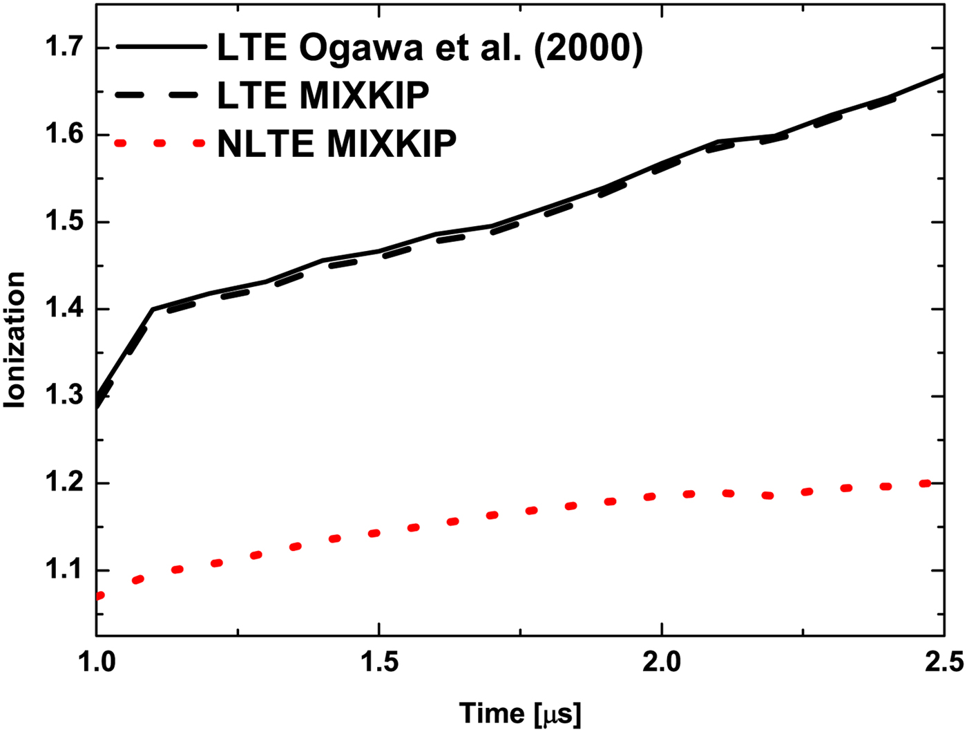
Fig. 2. Plasma ionization as a function of the evolution time. Ionization was calculated assuming LTE or NLTE conditions. The experimentalists curve with Eq. (12) is shown as a black solid line. Our calculations with MIXKIP: LTE (black dashed line), NLTE (red dotted line).
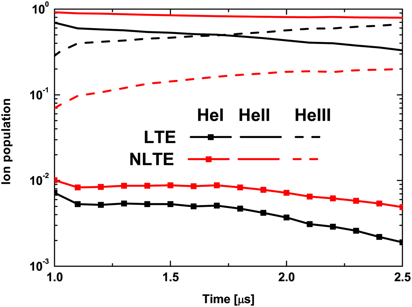
In Figure 3, the abundance of all plasma ions is shown. In both thermodynamic states, the plasma is composed mainly by HeII after the ignition, but its proportion decreases when discharge time increases as the proportion of HeIII grows up. HeI abundance is very low, always much smaller than HeII and HeIII ones. In NLTE case, HeII abundance is higher than HeIII one for the entire calculated range, not as in LTE case. In NLTE case also, HeI and HeII abundances are always higher than those calculated in LTE case. The difference between curves increase with time, so bound stopping power will be more important in NLTE case than in LTE case, specially the HeII one.

Fig. 3. Ionic abundance calculated using MIXKIP code in LTE conditions (black) or NLTE conditions (red) as a function of plasma evolution time. Scatter-solid, solid, and dashed lines correspond to HeI, HeII, and HeIII abundances, respectively.
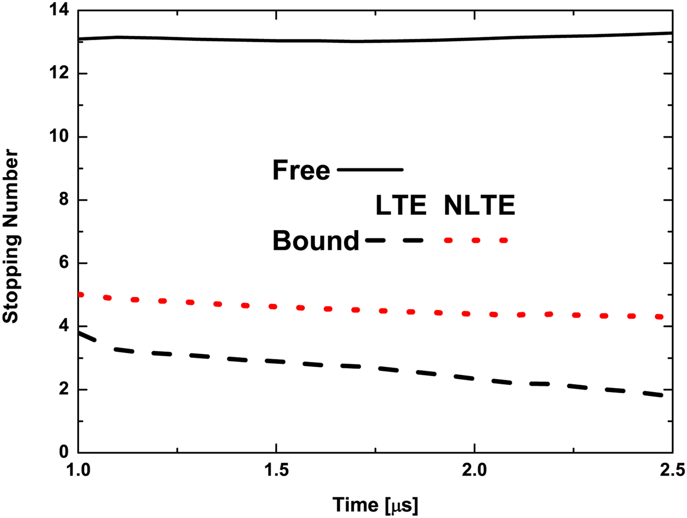
After studing ion abundances, the electron stopping number has been analyzed. This adimensional property provides information about the free, Eq. (9), and the bound, Eq. (10), electron contribution on the stopping power for a given condition of the target plasma, without regard to the properties of the ion beam. Free electron stopping number in LTE or NLTE thermodynamic states is the same, as this stopping number depends on the target by its dielectric function and by its free electron density, and both quantities are the same in both thermodynamic states. On the other hand, bound electron stopping number depends on the normalized abundances of the ions and their mean excitation energies, which at the same time rely upon the thermodynamic state. Therefore, diferences in the total stopping power in LTE and NLTE thermodynamic states are due to the bound electron contribution. From the calculations performed in this work, it has been obtained that the stopping number of free electrons is significantly higher than the one of bound electrons at any time after ignition of the target, see Figure 4. When the time increases, the bound stopping number also decreases, while the free one remains approximately constant. These behaviors are obtained when we consider both the LTE and NLTE thermodynamic states. Moreover, the bound stopping number calculated in NLTE thermodynamic state is always higher than in LTE, 20% at 1 µs and more than 50% at 2.5 µs after ignition. This is because HeI and HeII abundances are higher in NLTE state than in LTE one.

By their side, the experimentalists used the next expression to compute the stopping power (Ogawa et al., Reference Ogawa, Neuner, Kobayashi, Nakajima, Nishigori, Takayama, Iwase, Yoshida, Kojima and Hasegawa2000):
 $$- \displaystyle{{dE} \over {dX}} = \displaystyle{{4\pi Z^2} \over {v_{\rm p}^2}} n_{{\rm at}}\left[ {P\,{\rm ln}\left( {\displaystyle{{2v_{\rm p}^2} \over I}} \right) + Q\,{\rm ln}\left( {\displaystyle{{2v_{\rm p}^2} \over {\omega _{\rm p}}}} \right)} \right],$$
where P is the averaged electronic population for an atom in the target, and ωp = (4πn atQ)1/2 is the plasma frequency. Instead of using the dielectric formalism to estimate the free electron stopping number, the experimentalists use Bethe logarithm valid only for high energies. For bound electron stopping power, experimentalists use again Bethe logarithm, while our Eq. (3) makes an interpolation for high and low velocities. Ogawa et al. also calculated I as an average quantity for all electron shells and ion species, meanwhile in our model every shell of each species is considered.
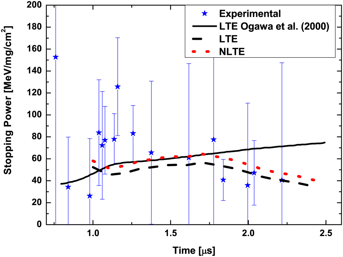
Finally, our total stopping power calculations in LTE or NLTE conditions are shown in Figure 5. It is observed that both curves have the same shape, more similar to the pattern of the measured data and cleary different to the theoretical curve from the experimentalists. First the stopping power decreases, then increases, and finally it decreases again following the experimental curve. In NLTE case, the calculations are higher than in LTE case approaching more to the data for all time mesurements. The main diffrences between the data and our calculations are obtained from 1 to 1.25 µs after ignition. From Figure 1, it is observed that the electron density shows large fluctuations in this tempotal interval, and this fact could explain these differences. Anyway, the experimental error bars are so large that are crossed by calculations in LTE or in NLTE conditions, then it is not easy to say if our model approximates better to experimental data in any of the two thermodynamic cases.

Fig. 5. Stopping power as function of plasma evolution time. Experimental data (blue scatter data) and calculations (black solid line) from Ogawa et al. (Reference Ogawa, Neuner, Kobayashi, Nakajima, Nishigori, Takayama, Iwase, Yoshida, Kojima and Hasegawa2000). Our calculations using Eq. (1) in LTE (black dashed line) or NLTE (red dotted line).
Conclusions
In this work, a comparison has been made between our theoretical method and experimental results for argon projectiles in a partially ionized helium plasma. Moreover, the thermodynamic state of the plasma has been also considered in the calculations through the ionic abundance and ionization of the plasma. For this work, LTE or NLTE has been considered.
About ionization, it can be seen that when LTE case is considered, it is higher than in NLTE case. Concerning ionic abundance, the most important abundance is HeII ion, which is even higher in NLTE case than in LTE one. On the other side, HeI abundance is always much lower than HeII and HeIII abundances, and HeIII abundance increases at large times when HeI and HeII abundances decrease. It is important to estimate correctly HeII and HeI abundances in order to calculate properly the bound stopping power.
Free electron stopping number are the same in both thermodynamic states. On the other hand, bound electron stopping number is higher in NLTE state than in LTE one, because of a lower target ionization and a higher HeII and HeI abundances. Therefore, diferences in the total stopping power in LTE and NLTE thermodynamic states are due to the bound electron contribution. When LTE conditions are assumed, total stopping power is lower than in NLTE conditions, but both curves are similar to the experimental data pattern. When also considering NLTE conditions, our calculations are a bit closer to Ogawa et al. calculations, although the curves do not follow the same direction at large times. Most of our results are within error experimental bars, but as experimental uncertainly is so considerable, it cannot be clearly said in which thermodynamic state the plasma is.
To summarize, it is worth to say that to estimate the stopping power of a plasma, it is important to know its thermodynamic state as it affects the ionization and the ionic abundances, therefore affects the free and bound plasma electron stopping power. In this specific case, experimental uncertainly makes difficult to establish if our model approximates better to experimental data in LTE or NLTE, and therefore to establish in which thermodynamic state the plasma is from an energy loss analysis.
Acknowledgments
L. G-G. is grateful to Ministerio de Educación for the Collaboration Grant to students at the University Departments for 2015–2016 academic year. This work has also been supported by the EUROfusion Consortium TASK AGREEMENT WPENR: Enabling Research IFE, Project No. AWP15-ENR-01/CEA-02 and by the Project of the Spanish Government with reference FIS2016-81019-P.