


1. INTRODUCTION
Simultaneous Q-switching (QS) and mode-locking (ML) of a laser oscillator, also referred to as transient ML or Q-switched mode-locking (QML), yields trains of ultra-short pulses during a Q-switch pulse envelope. Compared to a simple Q-switch, QML lead to considerably higher peak powers, and in contrast to the continuous waves (CW) ML, can still issue pulse energies in the mJ-range. It is thus a very elegant way to combine high pulse energies with ps-pulse durations from a laser oscillator.
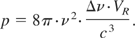
The first report on simultaneous ML and QS was published by Mocker and Collins (1965). They used a saturable absorber to mode-lock and Q-switch a ruby laser. Using saturable absorbers, QML often occurred when CW ML was actually desired, and is also referred to as QS instabilities. Thus the limits that separate the ML from the QML regime are well investigated (Kärtner et al., 1995; Hönninger et al., 1999).
Cr4+:YAG crystals are sometime bonded to the amplifier crystal (Zhang et al., 2005) and semiconductors are often used for QS and simultaneous ML of Nd-lasers (Chen & Tsai, 2001; Chen et al., 2001; Jeong et al., 1999). Also, nonlinear mirrors typically on the basis of second harmonic generation (SHG) and a dichroic mirror can be exploited to provide ML or QML operation (Jeong et al., 1999; Datta et al., 2004). Lamb and Damzen (1996) and Damzen et al. (1991) used a passive external cavity and a regenerative amplifier consisting of a conventional mirror, and a nonlinear mirror on the basis of the stimulated Brillouin scattering (SBS) to generate bandwidth, and to mode-lock the output from a narrow bandwidth pulsed oscillator. The laser discussed in this paper is a self starting SBS-laser oscillator where the SBS-mirror provides passive QS. The reflectivity of a nonlinear SBS-mirror stems from coherent scattering of light at a self-induced acoustic sound wave grating. Due to the movement of the acoustic wave, the reflected light experiences a Doppler-shift to lower frequencies that amounts to the resonance frequency of the acoustic wave, the so-called Brillouin frequency νB. Therefore, for each round trip, new longitudinal modes are generated that are coupled to the original modes. This ML effect of the SBS (Kawasaki et al., 1978; Lugovoi, 1983) was in our setup, supported by acousto optic modulation (AOM) in an additional component. Another feature of an SBS-mirror is its phase conjugating reflection which can be exploited for the compensation of phase distortions for high power master oscillator power amplifier system (MOPA-systems) (Rockwell, 1988) and oscillators (Ostermeyer et al., 1998), as well as for beam combining (Kong et al., 2005a; 2005b).
In this paper, the phase conjugation properties of the SBS-mirror are only of secondary importance. We will focus on the nonlinear reflectivity behavior of the SBS-mirror inside a resonator.
Section 2 of this paper reviews the schematic and the major output characteristics of the mode locked SBS-oscillator. In Sections 3 and 4, two models are presented to understand the dynamics of the laser oscillator better. The first model is a multimode rate equation model whereas the second model describes the laser dynamics with a resonator round trip model. In Section 5, the models are applied to study the influence of parameter variations on the duration of the pulses and the transient spectrum during the Q-switch envelope of the pulse.
The two models presented in Sections 3 and 4 are discussed with regard to their complementary character in the description of the mode locked SBS-oscillator by us in a recent publication (Kappe & Ostermeyer, 2006). There we validated our models by comparing the results of the models to output pulse structures of our realized laser oscillator. In this paper, we will elaborate on the evolution of the typical mode structure of the mode locked SBS-oscillator. Furthermore, we will investigate the impact of the SBS-material parameters phonon lifetime and Brillouin frequency on the mode spectrum, and pulse duration as well as the influence of the amplitude of loss modulation caused by AOM. The models enable us to vary single parameters to study their impact while holding all other parameters constant.
2. SCHEMATIC OF SBS-LASER OSCILLATOR WITH ADDITIONAL LOSS MODULATOR
A schematic of the setup for the SBS-laser to be discussed here is shown in Figure 1. The SBS-laser oscillator consists of two coupled cavities. A conventional start resonator is given by the output coupling mirror (OC) and the start resonator mirror Rstart. In this resonator configuration, the nonlinear SBS-mirror is situated in the middle of the start resonator, together with the OC, they compose the SBS-resonator. The laser oscillation starts in the start resonator when the SBS-mirror is still transparent. With growing intensity in the resonator, the SBS-reflectivity increases rapidly, and the oscillation switches to the SBS-resonator resulting in a Q-switch. The SBS-mirror consists of a gas cell (SF6 at 20 bar). Due to the movement of the accoustic wave, the reflected light experiences a shift to lower frequencies (Stokes-shift) that amounts to the frequency of the acoustic wave.

SBS-laser setup.
For the layout of the resonator, several aspects were considered: As mentioned before, the SBS-reflected light experiences a frequency shift. So if this light should be still accommodated in the resonator, the shift in frequency must be an integer multiple of the resonator's longitudinal mode spacing. In other words, the resonator length has to be a multiple of a fundamental resonator length, the Brillouin length LB which corresponds to the Brillouin frequency νB by LB = c/2·νB. Since the Brillouin frequency for SF6 at 20 bars is 240 MHz, the Brillouin length is 62.5 cm in this case.
The second aspect to be considered relates to the ML. If active ML is desired, the resonator's longitudinal mode spacing has also to be tuned to the modulation frequency of the AOM. In this case, it is 80 MHz, leading to a fundamental ML resonator length according to the ML of 187.5 cm. Since this is exactly three times the Brillouin length, the resonator length tuning for the SBS is always given if the ML condition is fulfilled. For optimal ML, this requirement has to be met by the SBS-resonator as well as the start resonator.
The matching of the longitudinal mode spacing for the start resonator is in this case also vital for the SBS-QS: The SBS-threshold for SF6 is too large to accomplish a self starting SBS-process in an oscillator from the acoustic noise (Meng & Eichler, 1991). An initial sound wave has to be build up in the SBS-material by Brillouin enhanced four wave mixing (BEFWM) (Scott & Ridley, 1989) of the back and forth traveling waves in the start resonator. The result can be a considerable reduction of the SBS-threshold for the incident light if again a multiple the longitudinal mode spacing of the start resonator modes matches the Brillouin frequency of the SBS-material. We chose the optical SBS-resonator length to equal the fundamental ML resonator length of 187.5 cm and the start resonator to have twice this length.
3. LASER SETUP OUTPUT PARAMTERS
A Nd:YAG rod is flash lamp pumped in a double elliptical cavity. The rod dimensions are 100 mm in length and 6.35 mm in diameter, and the doping level is 0.85%. The start resonator is formed by A concave output coupler with a reflectivity of ROC = 70% and a radius of curvature of 500 mm, and the plane start mirror with reflectivity Rstart varying according to the desired start resonator loss. As material for the nonlinear SBS-mirror, we used SF6 at 20 bars. The gas is contained in a 15 cm long brass tube with windows on either ends. Its rear window (farther away from the output coupler) is tilted to an angle of 5 degrees to prevent any interference between the windows and any disturbing back reflections in the region of SBS-reflection. The front window is a lens L1 with a focal length of 100 mm. Together with a second lens L2 of equal focal length that is placed outside the SBS-cell; it forms a telescope that generates a focus inside the SBS-cell (Fig. 1).
The SBS-cell with lens L1, lens L2, and the start resonator mirror are mounted in a way that they can be moved along the axis of the resonator. Thus the SBS-resonator length as well as the start-resonator length can be independently tuned. The distance between L1 and L2 is an additional free parameter that determines the position of the stability region, so that the pump power can be arbitrarily chosen within a range of a few kWs (Ostermeyer & Menzel, 1997; Ostermeyer et al., 1998). The pump power applied to the results presented below was around 3 kW. For these results, the laser head is pumped at a repetition rate of 180 Hz, the pump pulse duration is set to 300 μs. At the focal spot near the output coupler, a pinhole was placed to allow for transverse fundamental mode operation, and to prevent from focusing on the output coupler during buildup of the thermal lens (Menzel & Ostermeyer, 1998).
Figure 2 illustrates the measured intensity distribution of the mode-locked SBS-laser. The top graph shows a typical Q-switch pulse burst. Here the signal of the flash lamp pump pulse is super imposed onto the signal of the pulses. The apparent difference in amplitude of the pulse stems from a digitizing effect in the display of the short pulses on a comparatively long time scale. The bottom graph represents the mode-locked dynamics of a single Q-switch pulse.

Emission dynamics; top: Q-switch pulse train superimposed to flash lamp pump pulse, bottom: mode locked pulse train underneath Q-switch pulse envelope.
Bursts of up to 7 pulses could be generated within a pump pulse duration of 300 μs for an Rstart = 0.88. In this case, the average output power ranged between 2.0 W for one pulse per burst and 2.7 W for 7 pulses. In both cases, transverse fundamental mode operation is achieved. In the latter case, the Q-switch pulse energy was 2.3 mJ, the pulse duration (FWHM) was 117 ns. For Rstart = 0.32, one single pulse was received from each pump pulse. When the output power equals 2 W, Q-switch pulse energy of 11 mJ is achieved. The highest average output power for transverse fundamental mode operation was 6 W. Additional active ML did neither influence the Q-switch-pulse duration nor the Q-switch pulse energy significantly.
The output properties of the laser such as temporal Q-switch pulse spacing, pulse duration, and pulse energy are coupled. By changing the start resonator loss, all of these parameters are altered dependently. But by additionally varying the pump parameters, free parameters are added, and the mentioned output parameters can within boundaries be arbitrarily chosen. The large variability of this laser's temporal output properties was exploited for fundamental research in materials processing (Ostermeyer et al., 2005).
If active loss modulation is applied, we receive trains of ps-pulses with repetition rates of 80 MHz, where the envelope of the pulse train is shaped by the Q-switch (bottom graph in Fig. 2). The pulse energy of the ps-pulses is influenced by the start resonator reflectivity Rstart for two reasons. First, the Q-switch pulse energy increases with decreasing Rstart. Second, the Q-switch pulse width decreases with decreasing Rstart. So the Q-switch pulse energy is split into the smaller number of ps-pulses, the lower Rstart. Both effects lead to an increase in ps-pulse energy with decreasing Rstart. The ps-pulse energy ranges from 0.2 mJ to 2 mJ for start resonator reflectivity of 0.88 down to 0.32, respectively. Figure 3 shows the dependence of the mode-locked pulse energy on Rstart, where the number of mode-locked pulses per Q-switch pulse was gained by dividing the FWHM of the Q-switch pulses by the temporal spacing of the mode-locked pulses.

Pulse energy and number of mode-locked pulses per Q-switch as a function of the start resonator reflectivity Rstart.
The upper limit for the single pulse duration was directly measured with a fast photo diode (Thorlabs SV2) and an oscilloscope with 2 GHz bandwidth (Tectronix TDS 794D) to be 412 ps (see Fig. 2). For the highest achieved pulse energy of 2 mJ, this results in a peak power of almost 5 MW. The M2-number of the laser was determined with a beam propagation analyzer (Spiricon M2-200) to be better than 1.4.
4. MULTI-LONGITUDINAL-MODE RATE EQUATION MODEL
The laser rate equations are coupled differential equations to describe the evolution of the photon density and the inversion density, and their mutual interactions inside the cavity. They are the means of choice to calculate laser output dynamics (Siegman, 1986). However, the obtained photon density as a function of time is in fact the mean photon density inside the resonator. Therefore, dynamics on a time scale shorter than the resonator round trip time cannot be resolved, and additional efforts have to be made in order to display ML behavior in the calculations. The envelope of a mode-locked pulse is, on the one hand, determined by its mode spectrum, and on the other hand, by the phase relations of the respective modes. To comprise the ML dynamics in the simulation laser's spectrum, its transient behavior have to be included in the modeling. The spectrum can be considered by solving the laser rate equation for the photon density for each of the longitudinal modes individually. The laser rate equation for the photon density φn of the n-th mode of a mode-locked four-level laser neglecting the population of the pump band and the lower laser level is
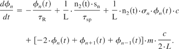
Here τR is the resonator decay time, l is the length of the laser active material, and L is the resonator length, n2 is the population density of the upper laser level, and σn is the frequency dependent stimulated emission cross section of the upper laser level. sn is the fraction of the spontaneous emission into the n-th mode. It contains the emission profile Sn and the total number p of resonant modes possible in the laser resonator volume VR (Koechner, 1999):

with
The first term on the right-hand side of Eq. (1) denotes the resonator losses followed by the terms for the spontaneous emission and the amplification. The fourth term describes an exchange of population between spectrally adjacent modes resulting from the modulation of depth m.
To include the nonlinear SBS-mirror into this model, several aspects have to be considered. First of all with increasing reflectivity of the SBS-mirror the oscillation switches from the start resonator to the SBS resonator. This switch affects on the one hand, the length, and on the other hand, the loss of the resonator that the revolving light experiences. Therefore, we have to substitute the resonator decay time τR and the resonator length L by corresponding expressions that depend on the time-dependent reflectivity of the SBS-mirror RSBS(t):
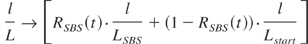
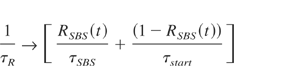
LSBS, Lstart, τSBS, Lstart are the lengths and decay times for the SBS and the start resonator, respectively.
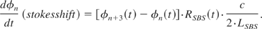
Furthermore, the Stokes shift which the reflected light experiences due to the movement of the reflecting sound wave has to be considered. The Stokes shift for SF6 at a pressure of 20 bars amounts to 240 MHz. This value is exactly three times the spectral spacing of the longitudinal modes of the SBS-resonator. Neglecting anti-Stokes- and higher Stokes-orders, we can describe the Stokes shift as a transfer of energy down the longitudinal mode scale of the SBS-resonator by three steps:
Including Eqs. (3) to (5) into Eq. (1), we obtain the time derivative of the photon density of the n-th mode:

Strictly speaking, this description applies only for those modes which can be accommodated in both resonators equally. The SBS-resonator modes are spaced by 80 MHz whereas the modes of the start-resonator which is twice as long are spaced by 40 MHz. Only every second start resonator mode will fit into the SBS-resonator. For the numerical calculations, the improper start-resonator modes will not be considered at all.
Due to the homogeneously broadened amplification bandwidth of Nd:YAG, the sum over all of the modes can be utilized to calculate the time derivative of the population of the upper laser level:
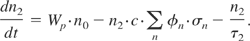
Wp denotes the pump rate and n0 and n2 are the density of dopant atoms and the population density of the upper laser level. It remains to implement the time dependent reflectivity RSBS(t) of the SBS-mirror. There is a model of the sound wave generation and the resulting reflectivity with temporal and spatial resolution for an external SBS-reflection (Menzel & Eichler, 1992; Afshaarvahid et al., 2001; Afshaarvahid & Munch, 2001). But we could not find any published model describing the sound wave generation and reflectivity with spatial resolution for the more complex case of a SBS-mirror inside a cavity. Here, we confine ourselves to a phenomenological description of the generation and decay of overall sound wave amplitude in the SBS-cell and its corresponding reflectivity Rstart(t). It is further assumed that the generation of the sound wave depends linearly on the intensity I(t) of the incident light:
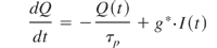
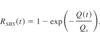
Eq. (9) is a more or less arbitrarily chosen function ranging from zero to unity describing the saturation behavior of the SBS-reflectivity. τp is the phonon lifetime, Q(t) is proportional to the sound wave amplitude, Qs describes the saturation sound wave amplitude, and g* is a Brillouin gain related parameter. g* and Qs will be used to fit the shape of the calculated Q-switch pulse envelopes to the experimental results. Their magnitudes determine if a Q-switch pulse occurs at all and govern the slope of the SBS-reflectivity. The latter influences the leading edge of the Q-switch pulse envelope. They do not influence the time at which the pulse occurs and therefore the pulse duration and pulse energy significantly. Also there is no direct relation to the ML. A third parameter that is used to fit the calculation to the experiment is the linear loss factor V of the SBS-resonator. It governs the resonator decay time and therefore the final edge of the pulse.
The resulting electrical field E(t) is obtained by the summation of the field contributions of all modes (En(t) ∼ [φ(t)]0.5), assuming that the phase factors are identical for all modes and can hence be set to zero. In this case, the intensity I(t) is given by:

The assumption that the phase factors for all modes are zero is identical to assuming perfect ML. In this case, the resulting mode-lock pulse is transform limited by the spectrum. Phase noise due to spontaneous emission and the SBS-bandwidth, as well as a mismatch between longitudinal mode spacing and modulation frequency are being neglected.
Another aspect that is not incorporated in this model is the propagation of light in the resonator. If we would start a calculation according to this model with just one mode occupied, it would yield three modes populated for the next time step due to the exchange term for the modulation. In the next but one time step already five modes would be populated notwithstanding the fact that the light would actually have to do one full round trip until it passes the modulator for a second time. The same argument applies for the Stokes shift as well what becomes most apparent when RSBS becomes unity. In this case, all the light will be shifted by three modes for each round trip, thus the spectrum is expected to be shifted as a whole, and the Stokes shift would not contribute to the generation of bandwidth in reality. In this model however, the Stokes shift is described as an exponential decay and growth where a constant percentage of the population of the respective mode is shifted in each time step. As we will see in Section 5, this description yields a generation of bandwidth even though RSBS approaches unity.
In the following section, we will refer to this model based on spectrally resolved rate equations as the frequency domain model since the ML dynamics are described in the frequency domain.
5. ROUND TRIP MODEL
The description of ML with rate equations for many longitudinal modes as presented in Section 4, yields dynamics on a ps-time scale that are strictly related to the spectrum of the intensity. It is a best case scenario since imperfections such as frequency mismatches and phase noise due to the statistical spontaneous emission process are left out. This section presents a model with a contrary approach by describing all occurring dynamics in the time domain. Spontaneous emission is assumed to be a continuous wave and the ML effect of the AOM is incorporated as a harmonic loss modulation. To display sub-round trip time dynamics, a spatial resolution of the photon density current along the axis of the resonator is introduced. Due to the propagation of the light this is equivalent to a temporal resolution.
The basic idea for this model is to display the photon density current at one certain spot in the resonator i.e., position 0 in Figure 4 in contrast to the mean photon density in the resonator that is considered in the rate equations. In order to compute the photon density current j(t) at a certain time t, we refer to the photon density current j(t − T) that was to be found here one round trip time T ago, and calculate all changes that the light has experienced during this round trip. In order to calculate the changes during this round trip, three intermediate steps will be taken corresponding to the positions 1–3 in the resonator indicated in Figure 4.

Time domain calculation scheme.
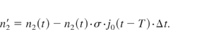
The first step would be to calculate the amplified photon density current j1 and the depleted inversion density n2′ after the first pass of the amplifier:
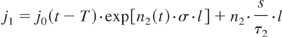
Again s is the fraction of the spontaneous emission into the laser mode. Strictly speaking, we would have to write j1(t − T + Δt01) where Δt01 refers to the delay time corresponding to the propagation from position 0 to position 1 (Fig. 4). But since this is only an intermediate step to illustrate the calculation procedure and since the exact times corresponding to these steps are of no relevance, this distinction is neglected here. Apart from that, the intensity is only recorded and displayed for position 0 anyways and the four calculation steps could just as well be merged into a single step.
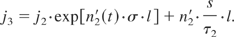
The expression for the inversion depletion is derived from the laser rate equations. Δt refers to the width of the time step that is calculated. The second step describes the harmonic loss modulation and linear resonator as well as output coupling losses:
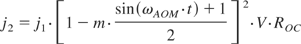
ωAOM is the modulation frequency of the AOM, V is the resonator round trip loss factor, and R0C is the output coupling reflectivity. What follows is a second pass through the amplifier now with the partially depleted inversion density n2′.
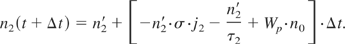
In the calculation of the inversion density for the next time step n2(t + Δt) expressions for the pump process and the spontaneous emission loss must be included:
Now we can obtain the photon density current j0 at the examined position by considering the transmission of the SBS-mirror in both directions:

jstart is the portion of the light that leaks through the SBS-mirror into the start resonator:

An equivalent description of the approach taken in this model is that we consider packages of light of length cΔt and let them propagate through the resonator and register all interactions with the optical devices. By doing this N = T/Δt times for N successive packages of light, we have completed a full resonator round trip and recorded the photon density current in the resonator with a spatial resolution corresponding to cΔt. This data will be the starting condition for the next round trip.
Apparently the propagation described by this model approximates the experimental setup described in Figure 1. This model describes a setup with the amplifier and the modulator situated at the position of the output coupler. So pumping and depletion by other fractions of the revolving light between the first and second pass through the amplifier remain unconsidered. Also the influence of the Stokes shift on the mode-locking is not taken into account.
6. APPLICATION OF THE MODELS
It was already found in one of our earlier publications (Ostermeyer et al., 1999) that longitudinal modes spaced by the Brillouin frequency of the used SBS-material dominate the longitudinal mode pattern. This changes if a loss modulator is used with a modulation frequency ωAOM smaller than the Brillouin frequency of the SBS-material 2πνB, like in our oscillator scheme and if the SBS-resonator in principle allows for mode separation frequencies c/2LSBS that equal this modulation frequency ωAOM. Figure 5 shows two typical mode spectra taken behind a Fabry Perot interferometer (FPI) of the SBS-oscillator with and without additional AOM operation. Figure 6 shows the evaluation of these interferograms. It can be clearly seen that the possible positions on the longitudinal mode grid that remain empty without AOM operation are filled when the AOM is switched on.

Fabry-Perot interferograms for the SBS-laser without (left) and with (right) active ML

Evaluation of longitudinal mode separation for mode structures of Fig. 5.
The rate equation model supports and explains this finding. Two different initial conditions have been considered, first, spontaneous emission into all modes within the line width of Nd:YAG and second, spontaneous emission into just the central longitudinal mode. In the first theoretical scenario, all possible longitudinal modes on the grid start oscillating regardless if the AOM is switched on or off. Whereas in the second scenario, bandwidth develops with time and without AOM, only the modes spaced by the Brillouin frequency get populated. Figure 7 shows the result of such a calculation for the second case for three different modulation amplitudes of the AOM. In this case, the oscillation starts with one longitudinal mode and it can be understood from the calculation that the AOM merely smears up the mode super grid between the positions that have been populated via the Stokes shift in the SBS mirror already. It also illustrates that the bandwidth generation of the mode locked SBS oscillator is mainly caused by the SBS Stokes shift and not by the loss modulation.

Calculated mode spectra according to the rate equation model for different amplitudes of the loss modulation at four different times (50 ns, 150 ns, 250 ns, 350 ns) during the Q-switch envelope.
Thus, it can be expected that the application of an SBS-material with a larger Brillouin frequency νB leads to a broader spectrum after the onset of the Q-switch. This in turn should provide the opportunity to generate shorter mode locked pulses. Figure 8 presents the calculated transient pulse spectra for four different Stokes shifts νB. The AOM loss modulation frequency is fixed at 80 MHz as in our experimental setup and the depth of modulation is 3%. As has been pointed out by us before (Kappe & Ostermeyer, 2006) when the Q-switch sets in the spectrum gets transient. It can be seen that the bandwidth indeed should get larger for SBS-materials with a higher Brillouin frequency νB. If the Brillouin frequency becomes very big as in the case of νB = 960 MHz, an AOM with 80 MHz modulation frequency and a loss modulation depth of 3% will not only be sufficient to fill the mode positions on the frequency grid between the Brillouin super grid. The result will be the occurrence of side pulses at a distance of 1/960 MHz ≈ 1 ns with amplitude of 5% of the main pulse peak intensity in this specific case.

Calculated transient mode spectra according to the rate equation model for four different Brillouin–frequencies νB.
The resulting duration of the mode locked pulses (evaluated at the peak of the Q-switch envelope) is plotted in Figure 9 as a function of the Brillouin frequency and inverse Brillouin frequency. The latter shows that there is a strict inverse linear dependence of the pulse duration and the Brillouin frequency. This is because the growing Brillouin frequency directly causes a proportionally growing bandwidth of the pulses.

Pulse duration evaluated from the calculated spectra from Fig. 8.
This seems to suggest working with SBS-material with a big Brillouin frequency in order to realize short pulse durations. In our theoretical numerical consideration, we have held the phonon lifetime artificially constant. However, if the phonon lifetime becomes too short compared to the SBS-resonator round trip time, the sound wave will decay and SBS will be inhibited. Damzen et al. (1991) found that for phonon lifetimes shorter than the fourth of the cavity round trip time laser action will cease (see Barrientos et al., 1995).
We finally investigate the variation of the phonon lifetime on the pulse duration. Again, in our investigation all other parameters are held constant. We investigated this dependence by using the round trip model, because it allows for faster computing times and contains all the features that are necessary to handle the problem qualitatively. Still, it especially allows for modeling a nonlinear mirror with a varying reflectivity. Since this model is not able to describe the bandwidth generation via the Stokes shift, the bandwidth is reduced and hence the mode locked pulses are somewhat longer in the following example. We learned from the Fabry Perot spectra and the simulations on the basis of the multi-longitudinal-mode rate equations model, that the emission starts from one dominant mode. Accordingly, we assume spontaneous emission into just one mode to be the starting condition for the time-domain model as well. Therefore the fraction s of spontaneous emission into the laser mode, which is in general the ratio between the number of laser modes pL and the number p of resonant modes possible in the laser resonator volume VR, becomes 1/p.
The mode-lock pulse duration is evaluated for different values of the phonon lifetime. A bi-stable like behavior results as can be gathered from the top part of Figure 10. For phonon lifetimes short compared to the resonator round trip time which is 12.5 ns in this example the pulse duration decreases by almost a factor of two.

Impact of Phonon lifetime on pulse duration (top) calculated according to the round trip model. The figures at the bottom show the evolution of the reflectivity of the SBS-mirror for three different phonon lifetimes marked in the top diagram.
The reason for this lies in the direct connection of the decay of the sound wave with the reflectivity of the SBS-mirror. If the phonon lifetime gets short compared to the round trip time the reflectivity varies distinctly. The model allows following up this behavior as depicted in the bottom diagrams of Figure 10. For long phonon lifetimes during the main part of the Q-switch envelope the SBS-reflectivity saturates on a high level. For short phonon lifetimes the SBS-reflectivity decays down to zero before it builds up with the arrival of the next pulse again. This strong variation of the SBS-reflectivity leads to a truncation of the edges of the pulse and hence a pulse shortening. It provides a second loss modulation beside the AOM. If this phase locking effect of the modulation in the SBS-reflectivity provides a perfect synchronization of the modes which are generated by the SBS-Stokes shift the AOM could be set aside. Unfortunately, neither the frequency domain nor the time domain model is presently capable of investigating this issue any further.
7. SUMMARY
Parameter variations of a mode locked SBS-laser oscillator have been investigated theoretically. The basis for this variation is an experimentally realized oscillator using an SBS-mirror based on SF6 at 20 bars that offers a wide variability of pulse structures. This stand alone oscillator is capable of providing pulses of 412 ps duration with average output powers of up to 6 W. The peak power of the pulses is adjustable up to 5 MW. The understanding of the longitudinal mode structure is the key to further improve the pulse parameters. To generate this understanding two complementary models have been considered, a multimode rate equation model and a round trip model.
The mode locked laser oscillator starts to oscillate with one longitudinal mode. Bandwidth in the sense of population of longitudinal modes is mainly generated due to the Stokes shift of the SBS-mirror when the light gets reflected round trip by round trip. The loss modulator (AOM) is merely responsible for the population of longitudinal modes on the frequency grid in between a Brillouin super grid. Shorter phonon lifetimes compared to the resonator round trip time will lead to shorter mode locked pulses and a larger Brillouin frequency also leads to shorter pulses via increased bandwidth generation.
To carry out these modifications in reality to further shorten the pulses though possible is more difficult compared to the direct theoretical treatment. The parameters that could be varied here independently from each other have to be found in a sound combination within the discrete islands of real materials.


