1. INTRODUCTION
As an ideal slow-wave structure with good dispersion characteristics and broad transmission band (Johnson et al., Reference Johnson, Everhart and Siegman1956), the tape helix was first used in the helical-type traveling wave tubes in the late 1940s (Pierce, Reference Pierce1950; Kompfner & Willanms, Reference Kompfner1947). Later, it was also employed in relativistic backward-wave oscillators for beam-wave interaction to excite microwave radiation (Kompfner et al., Reference Kompfner and Willianms1953; Tien, Reference Tien1954; Watkins & Ash, Reference Watkins and Ash1954). In the 1980s, the tape helix was introduced in the field of pulsed power technology to construct electron accelerator based on helical pulse forming line (HPFL), so that the pulse duration of accelerator was scaled up to several hundred ns range while the size of PFL decreased (Friedman et al., Reference Friedman, Limpaecher and Sirchis1988; Shidara et al., Reference Shidara, Akemoto and Yoshidda1991; Korovin et al., Reference Korovin, Gubanov, Gunin, Pegel and Stepchenko2001; Liu et al., Reference Liu, Li and Zhang2006, Reference Liu, Yin and Ge2007a, Reference Liu, Zhan, Zhang, Liu, Feng, Shu, Zhang and Wang2007b, Reference Liu, Cheng, Qian, Ge, Zhang and Wang2009; Cheng et al., Reference Cheng, Liu, Qian and Zhang2009).
Usually, the thin tape helix has deformation, and the tape helix can not be concentric with its metal shields, so that a strong dielectric support for the tape helix with enough thickness should be introduced (Swift-Hook, Reference Swift-Hook1958; Ghosh et al., Reference Ghosh, Jain and Basu1997; Agostino et al., Reference Agostino, Emma and Paoloni1998; Chernin et al., Reference Chernin, Antonsen and Levush1999; Kartikeyan et al., Reference Kartikeyan, Sinha and Bandopadhyay1999). In the tape helix slow-wave system, filling dielectric is also introduced to fill in the space inside the system for the purpose of good insulation (Swift-Hook, Reference Swift-Hook1958; Ghosh et al., Reference Ghosh, Jain and Basu1997; Agostino et al., Reference Agostino, Emma and Paoloni1998; Chernin et al., Reference Chernin, Antonsen and Levush1999; Kartikeyan et al., Reference Kartikeyan, Sinha and Bandopadhyay1999; Lopes & Motta, Reference Lopes and Motta2005). However, the support dielectric and filling dielectric are completely two different kinds of dielectrics, so that the discontinuity of dielectrics can cause obvious effects on the dispersion characteristics. Swift-Hook (Reference Swift-Hook1958) studied the dispersion characteristics of a thick tape helix in a glass tube, and different regions with dielectric characteristics were considered. However, no metal shield condition was considered in glass tube. Agostino et al. (Reference Agostino, Emma and Paoloni1998), Chernin et al. (Reference Chernin, Antonsen and Levush1999), and Kartikeyan et al. (Reference Kartikeyan, Sinha and Bandopadhyay1999) analyzed the effects of vane-loaded and bar-type support dielectrics on the tape helix system with an outer metal shield, but the vane-loaded approximation had an obvious error with experimental results (Kartikeyan et al., Reference Kartikeyan, Sinha and Bandopadhyay1999). Dialetis et al. (Reference Dialetis, Chernin and Antonsen2009), Datta and Kumar (Reference Datta and Kumar2009), and Datta et al. (Reference Datta, Naidu and Rao2010) analyzed the effects of multi-layer dielectrics in radial direction on the dispersion characteristics of the tape helix system, which only had an outer metal shield, and experimental results were in line with theoretical calculations. Furthermore, in order to improve the dispersion characteristics and obtain advantages in geometric size, a concentric inner metal shield should be introduced inside the tape helix in many situations (Ge et al., Reference Ge, Zhong and Qian2010), which causes more complicated boundary conditions. Ge et al. (Reference Ge, Zhong and Qian2010) improved dispersion characteristics and accomplished a more miniaturized relativistic backward-wave oscillator in L band, by introducing an air-core inner metal shield. And the extensively used helical Blumlein pulse forming line also has an inner metal shield (Liu et al., Reference Liu, Li and Zhang2006; Chen et al., Reference Chen, Liu and Zhang2009, Reference Chen, Liu and Zhang2010). By far, however, researches that are involved in the effects of radial dielectric discontinuity on the dispersion characteristics of the tape helix slow-wave system including two metal shields are still not adequate.
In this work, the electromagnetic field distribution of the tape helix slow-wave system of the electron accelerator with radial dielectric discontinuity and two metal shields was analyzed by accurate electromagnetic theory. The effects of dielectric discontinuity on the dispersion characteristics were studied in detail. Phase velocities, slow-wave coefficients, and electric lengths were calculated. The simulation and experimental results attested the theoretical analyses and many valuable conclusions were obtained for the first time, which showed great value on further study of tape helix slow-wave structure in HPFL and long pulse accelerator.
2. ELECTROMAGNETIC FIELDS AND DISPERSION EQUATION OF THE TAPE HELIX SLOW-WAVE SYSTEM
Figure 1 shows geometric structure of the tape helix slow-wave system that consists of an outer shield, tape helix, an inner shield, air-core cylindrical nylon support dielectric, and filling dielectric. The “infinitesimally thin” tape helix approximation is adopted in this work, as it is accurate if the work frequency is not high enough (Sensiper, Reference Sensiper1951, Reference Sensiper1955). Cylindrical coordinates (r × θ × z) are established along the axial direction (z) as Figure 1a shows that r and θ represent the radial and azimuthal direction, and r 1, r 2, r 3 represent the radii of the inner shield, tape helix, and the outer shield, respectively. The inner and outer radii of nylon support are a and r 2. ψ is the pitch angle of tape helix, while the pitch and tape width are p and δ, respectively. l 0 is the length of the infinitesimally thin tape in the axial direction. As Figure 1b shows, the filling dielectric and the nylon support have different relative permittivities as ɛr1 and ɛr2, dielectric discontinuity phenomenon in the radial direction occurs. Considering the different boundary conditions of the slow-wave system, the inner and outer shields are ideal conductors. So, only three regions are separated to analyze the electromagnetic fields distribution, such as region I (r 1 < r < a), region II (a < r < r 2) and region III (r 2 < r < r 3). The permittivity and permeability of free space are ɛ0 and μ0, respectively. The filling dielectric is the same in regions II and III, and its permittivity and permeability are ɛ1 and μ1, while permittivity and permeability of nylon support in region II are ɛ2 and μ2, respectively. Then ɛi = ɛriɛ0 × μi = μriμ0 (I = 1, 2).

Fig. 1. (Color online) The tape helix slow-wave system with a cylindrical support insulator, filling dielectric and two metal shields. (a) Geometric structure of the tape helix slow-wave system. (b) Cross section of the slow-wave system.
The electromagnetic field and its excitation surface current density J are both in periodical distribution, due to the azimuthal periodicity and helical symmetry of the tape helix. If l 0 ≫ r 2, the electromagnetic field and J both consist of their own infinite terms of spatial harmonic components, according to the Floquet theorem (Sensiper, Reference Sensiper1951). In these spatial harmonics, the axial phase constant βn of the n th harmonic has relation with β0 (phase constant of the zero harmonic) as βn = β0 + 2πn/p. By solving the Maxwell equations, the analytical solutions of electromagnetic field in the three specified regions are as follows.
Region I (r 1 < r < a):
![\left\{{\matrix{ \matrix{E_{1z} = e^{ - j\lpar {\rm \beta} _0 z - {\rm \omega} t\rpar } \sum\limits_{n = - \infty }^{ + \infty } {} \hfill \lsqb A_{1n} I_n \lpar {\rm \gamma} _n r\rpar + A_{2n} K_n \lpar {\rm \gamma} _n r\rpar \rsqb e^{ - jn\lpar 2{\rm \pi} z/p - {\rm \theta} \rpar } \hfill} \hfill \cr \matrix{E_{1r} = e^{ - j\lpar {\rm \beta} _0 z - {\rm \omega} t\rpar } \sum\limits_{n = - \infty }^{ + \infty } {} \hfill \Bigg [ \displaystyle{{\,j{\rm \beta} _n } \over {{\rm \gamma} _n }}\lpar A_{1n} I_n^\prime \lpar {\rm \gamma} _n r\rpar + A_{2n} K_n^\prime \lpar {\rm \gamma} _n r\rpar \rpar \hfill \cr \hskip25pt- \displaystyle{{{\rm \omega} {\rm \mu} _1 n} \over {{\rm \gamma} _n^2 r}} \lpar A_{3n} I_n \lpar {\rm \gamma} _n r\rpar + A_{4n} K_n \lpar {\rm \gamma} _n r\rpar \rpar \Bigg ] e^{ - jn\lpar 2{\rm \pi} z/p - {\rm \theta} \rpar } \hfill} \hfill \cr \matrix{E_{1{\rm \theta} } = e^{ - j \lpar {\rm \beta} _0 z - {\rm \omega} t\rpar } \sum\limits_{n = - \infty }^{ + \infty } {} \hfill \Bigg [ \displaystyle{{ - n{\rm \beta} _n } \over {{\rm \gamma} _n^2 r}}\lpar A_{1n} I_n \lpar {\rm \gamma} _n r\rpar + A_{2n} K_n \lpar {\rm \gamma} _n r\rpar \rpar \hfill \cr \hskip25pt- \displaystyle{{\,j{\rm \omega} {\rm \mu} _1 } \over {{\rm \gamma} _n }}\lpar A_{3n} I_n^\prime \lpar {\rm \gamma} _n r\rpar + A_{4n} K_n^\prime \lpar {\rm \gamma} _n r\rpar \rpar \Bigg ] e^{ - jn\lpar 2{\rm \pi} z/p - {\rm \theta} \rpar } \hfill} \hfill \cr \matrix{H_{1z} = e^{ - j\lpar {\rm \beta} _0 z - {\rm \omega} t\rpar } \sum\limits_{n = - \infty }^{ + \infty } {} \hfill \lsqb A_{3n} I_n \lpar {\rm \gamma} _n r\rpar + A_{4n} K_n \lpar {\rm \gamma} _n r\rpar \rsqb e^{ - jn\lpar 2{\rm \pi} z/p - {\rm \theta} \rpar } \hfill} \hfill \cr \matrix{H_{1r} = e^{ - j\lpar {\rm \beta} _0 z - {\rm \omega} t\rpar } \sum\limits_{n = - \infty }^{ + \infty } {} \hfill \Bigg [ \displaystyle{{{\rm \omega} {\rm \varepsilon} _1 n} \over {{\rm \gamma} _n^2 r}}\lpar A_{1n} I_n \lpar {\rm \gamma} _n r\rpar + A_{2n} K_n \lpar {\rm \gamma} _n r\rpar \rpar \hfill \cr \quad \qquad+ \displaystyle{{\,j{\rm \beta} _n } \over {{\rm \gamma} _n }}\lpar A_{3n} I_n^\prime \lpar {\rm \gamma} _n r\rpar + A_{4n} K_n^\prime \lpar {\rm \gamma} _n r\rpar \rpar \Bigg ] e^{ - jn\lpar 2{\rm \pi} z/p - {\rm \theta} \rpar } \hfill} \hfill \cr \matrix{H_{1{\rm \theta} } = e^{ - j\lpar {\rm \beta} _0 z - {\rm \omega} t\rpar } \sum\limits_{n = - \infty }^{ + \infty } {} \hfill \Bigg [ \displaystyle{{\,j{\rm \omega} {\rm \varepsilon} _1 } \over {{\rm \gamma} _n }}\lpar A_{1n} I_n^\prime \lpar {\rm \gamma} _n r\rpar + A_{2n} K_n^\prime \lpar {\rm \gamma} _n r\rpar \rpar \hfill \cr \quad\qquad- \displaystyle{{{\rm \beta} _n n} \over {{\rm \gamma} _n^2 r}}\lpar A_{3n} I_n \lpar {\rm \gamma} _n r\rpar + A_{4n} K_n \lpar {\rm \gamma} _n r\rpar \rpar \Bigg ] e^{ - jn\lpar 2{\rm \pi} z/p - {\rm \theta} \rpar } \hfill} \hfill \cr } } \right..](https://static.cambridge.org/binary/version/id/urn:cambridge.org:id:binary-alt:20160626081037-32595-mediumThumb-S0263034611000826_eqn1.jpg?pub-status=live)
Region II (a < r < r 2):
![\left\{{\matrix{ \matrix{E_{2z} = e^{ - j\lpar {\rm \beta} _0 z - {\rm \omega} t\rpar } \sum\limits_{n = - \infty }^{ + \infty } {} \lsqb G_{1n} I_n \lpar {\rm \gamma} _n r\rpar + G_{2n} K_n \lpar {\rm \gamma} _n r\rpar \rsqb e^{ - jn\lpar 2{\rm \pi} z/p - {\rm \theta} \rpar } \hfill} \hfill\cr \hskip-24pt \matrix{E_{2r} = e^{ - j\lpar {\rm \beta} _0 z - {\rm \omega} t\rpar } \sum\limits_{n = - \infty }^{ + \infty } {} \hfill \Bigg [ \displaystyle{{\,j{\rm \beta} _n } \over {{\rm \gamma} _n }}\lpar G_{1n} I_n^\prime \lpar {\rm \gamma} _n r\rpar + G_{2n} K_n^\prime \lpar {\rm \gamma} _n r\rpar \rpar \hfill \cr \qquad \;\,- \displaystyle{{{\rm \omega} {\rm \mu} _2 n} \over {{\rm \gamma} _n^2 r}}\lpar G_{3n} I_n \lpar {\rm \gamma} _n r\rpar + G_{4n} K_n \lpar {\rm \gamma} _n r\rpar \rpar \Bigg ] e^{ - jn\lpar 2{\rm \pi} z/p - {\rm \theta} \rpar } \hfill} \cr \hskip-24pt \matrix{E_{2{\rm \theta} } = e^{ - j\lpar {\rm \beta} _0 z - {\rm \omega} t\rpar } \sum\limits_{n = - \infty }^{ + \infty } {} \hfill \Bigg [ \displaystyle{{ - n{\rm \beta} _n } \over {{\rm \gamma} _n^2 r}}\lpar G_{1n} I_n \lpar {\rm \gamma} _n r\rpar + G_{2n} K_n \lpar {\rm \gamma} _n r\rpar \rpar \hfill \cr \quad\quad\;\,- \displaystyle{{\,j{\rm \omega} {\rm \mu} _2 } \over {{\rm \gamma} _n }}\lpar G_{3n} I_n^\prime \lpar {\rm \gamma} _n r\rpar + G_{4n} K_n^\prime \lpar {\rm \gamma} _n r\rpar \rpar \Bigg ] e^{ - jn\lpar 2{\rm \pi} z/p - {\rm \theta} \rpar } \hfill}\cr {H_{2z} = e^{ - j\lpar {\rm \beta} _0 z - {\rm \omega} t\rpar } \sum\limits_{n = - \infty }^{ + \infty } }\hfill {\Bigg [ G_{3n} I_n \lpar {\rm \gamma} _n r\rpar + G_{4n} K_n \lpar {\rm \gamma} _n r\rpar \rsqb e^{ - jn\lpar 2{\rm \pi} z/p - {\rm \theta} \rpar } } \hfill \cr \matrix{H_{2r} = e^{ - j\lpar {\rm \beta} _0 z - {\rm \omega} t\rpar } \sum\limits_{n = - \infty }^{ + \infty } {} \hfill \Bigg [ \displaystyle{{{\rm \omega} {\rm \varepsilon} _2 n} \over {{\rm \gamma} _n^2 r}}\lpar G_{1n} I_n \lpar {\rm \gamma} _n r\rpar + G_{2n} K_n \lpar {\rm \gamma} _n r\rpar \rpar \hfill \cr \hskip28pt + \displaystyle{{\,j{\rm \beta} _n } \over {{\rm \gamma} _n }}\lpar G_{3n} I_n^\prime \lpar {\rm \gamma} _n r\rpar + G_{4n} K_n^\prime \lpar {\rm \gamma} _n r\rpar \rpar \Bigg ] e^{ - jn\lpar 2{\rm \pi} z/p - {\rm \theta} \rpar } \hfill} \cr \matrix{H_{2{\rm \theta} } = e^{ - j\lpar {\rm \beta} _0 z - {\rm \omega} t\rpar } \sum\limits_{n = - \infty }^{ + \infty } {} \hfill \Bigg [ \displaystyle{{\,j{\rm \omega} {\rm \varepsilon} _2 } \over {{\rm \gamma} _n }}\lpar G_{1n} I_n^\prime \lpar {\rm \gamma} _n r\rpar + G_{2n} K_n^\prime \lpar {\rm \gamma} _n r\rpar \rpar \hfill \cr \hskip28pt - \displaystyle{{{\rm \beta} _n n} \over {{\rm \gamma} _n^2 r}}\lpar G_{3n} I_n \lpar {\rm \gamma} _n r\rpar + G_{4n} K_n \lpar {\rm \gamma} _n r\rpar \rpar \Bigg ] e^{ - jn\lpar 2{\rm \pi} z/p - {\rm \theta} \rpar } \hfill} \cr } }. \right.](https://static.cambridge.org/binary/version/id/urn:cambridge.org:id:binary-alt:20160626081135-22891-mediumThumb-S0263034611000826_eqn2.jpg?pub-status=live)
Region III (r 2 < r < r 3)
![\left\{{\matrix{ \matrix{E_{3z} = e^{ - j\lpar {\rm \beta} _0 z - {\rm \omega} t\rpar } \sum\limits_{n = - \infty }^{ + \infty } {} \hfill \big [ B_{1n} I_n \lpar {\rm \gamma} _n r\rpar + B_{2n} K_n \lpar {\rm \gamma} _n r\rpar \rsqb e^{ - jn\lpar 2{\rm \pi} z/p - {\rm \theta} \rpar } \hfill} \cr \hskip-1.6pc\matrix{E_{3r} = e^{ - j\lpar {\rm \beta} _0 z - {\rm \omega} t\rpar } \sum\limits_{n = - \infty }^{ + \infty } {} \hfill \Bigg [ \displaystyle{{\,j{\rm \beta} _n } \over {{\rm \gamma} _n }}\lpar B_{1n} I_n^\prime \lpar {\rm \gamma} _n r\rpar + B_{2n} K_n^\prime \lpar {\rm \gamma} _n r\rpar \rpar \hfill \cr \hskip27pt - \displaystyle{{{\rm \omega} {\rm \mu} _1 n} \over {{\rm \gamma} _n^2 r}}\lpar B_{3n} I_n \lpar {\rm \gamma} _n r\rpar + B_{4n} K_n \lpar {\rm \gamma} _n r\rpar \rpar \Bigg ] e^{ - jn\lpar 2{\rm \pi} z/p - {\rm \theta} \rpar } \hfill} \cr \hskip-1pc\matrix{E_{3{\rm \theta} } = e^{ - j\lpar {\rm \beta} _0 z - {\rm \omega} t\rpar } \sum\limits_{n = - \infty }^{ + \infty } {} \hfill \Bigg [ \displaystyle{{ - n{\rm \beta} _n } \over {{\rm \gamma} _n^2 r}}\lpar B_{1n} I_n \lpar {\rm \gamma} _n r\rpar + B_{2n} K_n \lpar {\rm \gamma} _n r\rpar \rpar \hfill \cr \hskip25pt - \displaystyle{{\,j{\rm \omega} {\rm \mu} _1 } \over {{\rm \gamma} _n }}\lpar B_{3n} I_n^\prime \lpar {\rm \gamma} _n r\rpar + B_{4n} K_n^\prime \lpar {\rm \gamma} _n r\rpar \rpar \Bigg ] e^{ - jn\lpar 2{\rm \pi} z/p - {\rm \theta} \rpar } \hfill} \cr \hskip-1pt \matrix{H_{3z} = e^{ - j\lpar {\rm \beta} _0 z - {\rm \omega} t\rpar } \sum\limits_{n = - \infty }^{ + \infty } {} \hfill \big [ B_{3n} I_n \lpar {\rm \gamma} _n r\rpar + B_{4n} K_n \lpar {\rm \gamma} _n r\rpar \rsqb e^{ - jn\lpar 2{\rm \pi} z/p - {\rm \theta} \rpar } \hfill} \cr \hskip-1pc\matrix{H_{3r} = e^{ - j\lpar {\rm \beta} _0 z - {\rm \omega} t\rpar } \sum\limits_{n = - \infty }^{ + \infty } {} \hfill \Bigg [ \displaystyle{{{\rm \omega} {\rm \varepsilon} _1 n} \over {{\rm \gamma} _n^2 r}}\lpar B_{1n} I_n \lpar {\rm \gamma} _n r\rpar + B_{2n} K_n \lpar {\rm \gamma} _n r\rpar \rpar \hfill \cr \hskip28pt + \displaystyle{{\,j{\rm \beta} _n } \over {{\rm \gamma} _n }}\lpar B_{3n} I_n^\prime \lpar {\rm \gamma} _n r\rpar + B_{4n} K_n^\prime \lpar {\rm \gamma} _n r\rpar \rpar \Bigg ] e^{ - jn\lpar 2{\rm \pi} z/p - {\rm \theta} \rpar } \hfill} \cr \hskip-1pc\matrix{H_{3{\rm \theta} } = e^{ - j\lpar {\rm \beta} _0 z - {\rm \omega} t\rpar } \sum\limits_{n = - \infty }^{ + \infty } {} \hfill \Bigg [ \displaystyle{{\,j{\rm \omega} {\rm \varepsilon} _1 } \over {{\rm \gamma} _n }}\lpar B_{1n} I_n^\prime \lpar {\rm \gamma} _n r\rpar + B_{2n} K_n^\prime \lpar {\rm \gamma} _n r\rpar \rpar \hfill \cr \hskip28pt - \displaystyle{{{\rm \beta} _n n} \over {{\rm \gamma} _n^2 r}}\lpar B_{3n} I_n \lpar {\rm \gamma} _n r\rpar + B_{4n} K_n \lpar {\rm \gamma} _n r\rpar \rpar \Bigg ] e^{ - jn\lpar 2{\rm \pi} z/p - {\rm \theta} \rpar } \hfill} \cr } }. \right.](https://static.cambridge.org/binary/version/id/urn:cambridge.org:id:binary-alt:20160626081148-29576-mediumThumb-S0263034611000826_eqn3.jpg?pub-status=live)
In Regions I–III, j is the unit of the imaginary number, n is the order number of the spatial harmonic, and ω is the angular frequency of the n th harmonic. Usually, condition βn ≫ ω is satisfied in the low frequency band, so that the phase constant γn of the transverse direction in different regions can be considered as the same. A 1n-A 4n, G 1n-G 4n, and B 1n-B 4n are 12 field coefficients that need to be calculated. I n and K n are the modified Bessel functions of the first and second kind, respectively. k i is the angular wave number (subscript i = 1, 2, 3) that corresponds to the three specified regions, and k i2 = ω2ɛi μi, γn2 = βn2 − k i2.
In Figure 1a, if δ ≪ p, the surface current that flows through the tape helix almost has the same distribution in the direction along the tape width (Sensiper, Reference Sensiper1951, Reference Sensiper1955). As the source of the electromagnetic field, the excitation surface current on the tape helix has many distribution models. In this work, the current model in reference (Sensiper, Reference Sensiper1951, Reference Sensiper1955) is adopted. That is to say, (1) the amplitude of surface current density (J 0) keeps the same on the tape helix; (2) in the gaps between the tape turns, J 0 = 0; (3) the phase constant plane of the helical surface current density is normal to the axial direction; (4) no current flows normal to the helical direction. The surface current density consists of two components, of which one is in parallel with the helical direction (J ‖) and the other is normal to the helical direction (J ⊥ = 0). Then, J ‖ can also be calculated by Floquet theorem as (Sensiper, Reference Sensiper1951)
If the inner and outer shields are ideal conductors, and the nylon support and filling dielectric are both ideal dielectrics (no losses need to be considered), the boundary conditions of the tape helix slow-wave system are as

By use of Eqs. (1)–(3) and the first 12 conditions in Eq. (5), the 12 field coefficients can be calculated as
![\left\{\matrix{G_{1n} = \displaystyle{j{\rm \gamma}_n J_{\parallel n} \over \rm \omega} \hfill \cr \qquad \qquad \displaystyle{[\cos \lpar {\rm \psi} \rpar - {\rm \beta}_n n\sin \lpar {\rm \psi} \rpar /\lpar {\rm \gamma} _n^2 r_2 \rpar] \lpar I_{n2} K_{n3} - I_{n3} K_{n2} \rpar \over \matrix{{\rm \varepsilon}_2 \lpar I_{n2}^{\prime} + a_1 K_{n2}^{\prime} \rpar \lpar I_{n2} K_{n3} - I_{n3} K_{n2} \rpar \hfill \cr - {\rm \varepsilon}_1 \lpar I_{n2} + a_1 K_{n2} \rpar \lpar I_{n2}^{\prime} K_{n3} - I_{n3} K_{n2}^{\prime} \rpar}} \hfill \cr G_{3n} = {\matrix{J_{\parallel n} \sin \lpar {\rm \psi} \rpar \lpar I_{n2}^{\prime} K_{n3}^{\prime} - I_{n3}^{\prime} K_{n2}^{\prime} \rpar} \over \matrix{\lpar I_{n2} + a_2 K_{n2} \rpar \lpar I_{n2}^{\prime} K_{n3}^{\prime} - I_{n3}^{\prime} K_{n2}^{\prime} \rpar \hfill \cr - {{\rm \mu}_2 \over {\rm \mu}_1} \lpar I_{n2}^{\prime} + a_2 K_{n2}^{\prime} \rpar \lpar I_{n2} K_{n3}^{\prime} - I_{n3}^{\prime} K_{n2} \rpar \hfill}} \hfill \cr G_{2n} = a_1 G_{1n} \comma \; G_{4n} = a_2 G_{3n} \hfill \cr A_{1n} = {G_{1n} I_{na} + G_{2n} K_{na} \over I_{na} - I_{n1} K_{na} /K_{n1}}\comma \; \hfill \cr A_{3n} = {{\rm \mu}_2 \over {\rm \mu}_1} {\lpar G_{3n} I_{na}^{{\prime}} + G_{4n} K_{na}^{{\prime}} \rpar \over \lpar I_{na}^{{\prime}} - I_{n1}^{\prime} K_{na}^{\prime} /K_{n1}^{\prime} \rpar} \hfill \cr A_{2n} = - A_{1n} I_{n1} /K_{n1} \comma \; A_{4n} = - A_{3n} I_{n1}^{\prime} /K_{n1}^{\prime} \hfill \cr B_{1n} = {I_{n2} + a_1 K_{n2} \over I_{n2} - I_{n3} K_{n2} /K_{n3}} G_{1n} \comma \; \hfill \cr B_{3n} = {{\rm \mu}_2 \over {\rm \mu}_1} {\lpar I_{n2}^{\prime} + a_2 K_{n2}^{\prime} \rpar \over \lpar I_{n2}^{\prime} - I_{n3}^{\prime} K_{n2}^{\prime} /K_{n3}^{\prime} \rpar} G_{3n} \hfill \cr B_{2n} = - {I_{n3} \over K_{n3}} B_{1n} \comma \; B_{4n} = { - I_{n3}^{\prime} \over K_{n3}^{\prime}} B_{3n} \hfill} \right..](https://static.cambridge.org/binary/version/id/urn:cambridge.org:id:binary-alt:20160626081033-84557-mediumThumb-S0263034611000826_eqn6.jpg?pub-status=live)
In Eq. (6), I n1, I n2, I na, and I n3 are the simplified forms of I n(γnr 1), I n(γnr 2), I n(γna), and I n(γnr 3), respectively, so do K n1, K n2, K na, and K n3. I n2′ represents the derivative of I n(γnr) to γnr when r = r 2, so does K n2′. At last, the transmitted slow waves in the slow-wave system are determined by the electromagnetic fields shown as Eqs. (1)–(3). In Eq. (6), a 1 and a 2 are parameters for simplification and their forms are as

According to Eqs. (2) and (5), the dispersion equation of the tape helix slow-wave system with dielectric discontinuity and two metal shields can be obtained as

In Eq. (8), J ‖nJ ‖n* can be substituted by sin2(nπδ/p)/(nπδ/p)2 (Sensiper, Reference Sensiper1951). The dispersion equation consists of infinite terms of Bessel functions.
3. DISPERSION RELATION AND SLOW-WAVE COEFFICIENT
Usually, the tape helix slow-wave structure is used for pulse forming line (PFL). The helical Blumlein PFL has the same structure as shown in Figure 1, and it is a device that outputs square (or quasi-square) voltage pulses for the accelerator with pulse duration ranging from dozens of ns to several hundred ns. These square pulses correspond to a work band that is less than 10 MHz. Under this low-frequency condition, the zero harmonic determines the dispersion characteristics of the helical Blumlein PFL. Select the zero term in Eq. (8) and equate it to 0, and the dispersion equation of the zero spatial harmonic can be obtained. Two different kinds of independent roots are obtained by solving this dispersion equation. And these roots just correspond to the dispersion relation of the zero harmonic as shown in Eq. (9).

In Eq. (9), a 10 and a 20 are parameters for simplification, and γ02 = β02(γ0) − ω02(γ0)ɛi μi. If the pitch angle ψ is large enough, the slow-wave coefficient p li = v ph/c i << 1 (c i is the light speed in different dielectric regions), and βn >> k, so that the approximation γ02 = β02 is accurate. As the periodical slow-wave structure has periodical dispersion curve, we employ ω~βp as the coordinates to explain the dispersion curve of the system. Actually, dispersion relation Eq. (9) shows the dispersion characteristics of the helical slow-wave system in the first ‘Brillouin zone’ (−π < β0p < π). Because βn = β0 + 2πn/p, the periodical dispersion relation of the helical slow-wave system is as
As the dispersion characteristics are almost determined by the zero harmonic at low frequency band, the parameters of the zero spatial harmonic such as phase velocity v ph0, slow-wave coefficient p l0, group velocity v g0 and electric length τ0′, are shown as Eq. (11) according to Eq. (9).
![\left\{{\matrix{ {v_{\,ph0} \lpar {\rm \gamma} _0 \rpar =\displaystyle{{{\rm \omega} _0 \lpar {\rm \gamma} _0 \rpar } \over {{\rm \beta} _0 \lpar {\rm \gamma} _0 \rpar }}=\displaystyle{{\cot \lpar {\rm \psi} \rpar } \over {\sqrt {{\rm \varepsilon} _i {\rm \mu} _i } }}\Big [ \displaystyle{g \over {T_0 \lpar {\rm \gamma} _0 \rpar }}+g^2 \cot \lpar {\rm \psi} \rpar ^2 \Big ] ^{1/2} } \cr {v_{g0} \lpar {\rm \gamma} _0 \rpar =\displaystyle{{d{\rm \omega} _0 \lpar {\rm \gamma} _0 \rpar } \over {d{\rm \beta} _0 \lpar {\rm \gamma} _0 \rpar }} \comma \; {\rm \tau} _0^{\prime}=l_0 /v_{\,ph0} \lpar {\rm \gamma} _0 \rpar } \cr {\,p_{l0} \lpar {\rm \gamma} _0 \rpar =v_{\,ph0} \lpar {\rm \gamma} _0 \rpar \sqrt {{\rm \varepsilon} _i {\rm \mu} _i }\comma \; \lpar i=1\comma \; 2\comma \; 3\rpar } \cr } } \right..\eqno\lpar 11\rpar](https://static.cambridge.org/binary/version/id/urn:cambridge.org:id:binary:20151021100151072-0360:S0263034611000826_eqn11.gif?pub-status=live)
In Eq. (11), factor g = ɛiμi/ɛ2μ2. Obviously, v ph0, p l0 and τ0′ are functions to γ0 in the first Brillouin zone of the dispersion curve, which show the effects of dispersion of helical slow-wave system on these important parameters. If the dielectric inside the system is continuous, the homogeneous dielectric corresponds to g = 1, otherwise, g ≠ 1. Factor g shows the effects of dielectric discontinuity on the phase velocity and dispersion characteristics of the tape helix slow-wave system.
4. EFFECTS OF SUPPORT DIELECTRIC ON THE DISPERSION CHARACTERISTICS OF THE TAPE HELIX SLOW-WAVE SYSTEM
In order to study the effects of dielectric discontinuity on the dispersion characteristics, a tape helix slow-wave system was produced, according to the geometric structure in Figure 1. The unifilar tape helix and its nylon support are shown as Figure 2. The Helix was formed by a copper tape (thickness at 0.2 mm) winding around the cylindrical nylon support. The geometric parameters of the slow-wave system including two metal shields are shown in Table 1. De-ionized water filled in the PFL as filling dielectric, and its relative permittivity and permeability were ɛr1 = 81.5 and μr1 = 1, respectively. The relative permittivity and permeability of nylon were ɛr2 = 4.5 and μr2 = 1. The thickness of the support dielectric d = r 2-a.

Fig. 2. (Color online) Helical slow-wave structure based on tape helix.
Table 1. Geometric parameters of the produced tape helix slow-wave system with nylon support
4.1. Dispersion Characteristics of the Spatial Harmonics
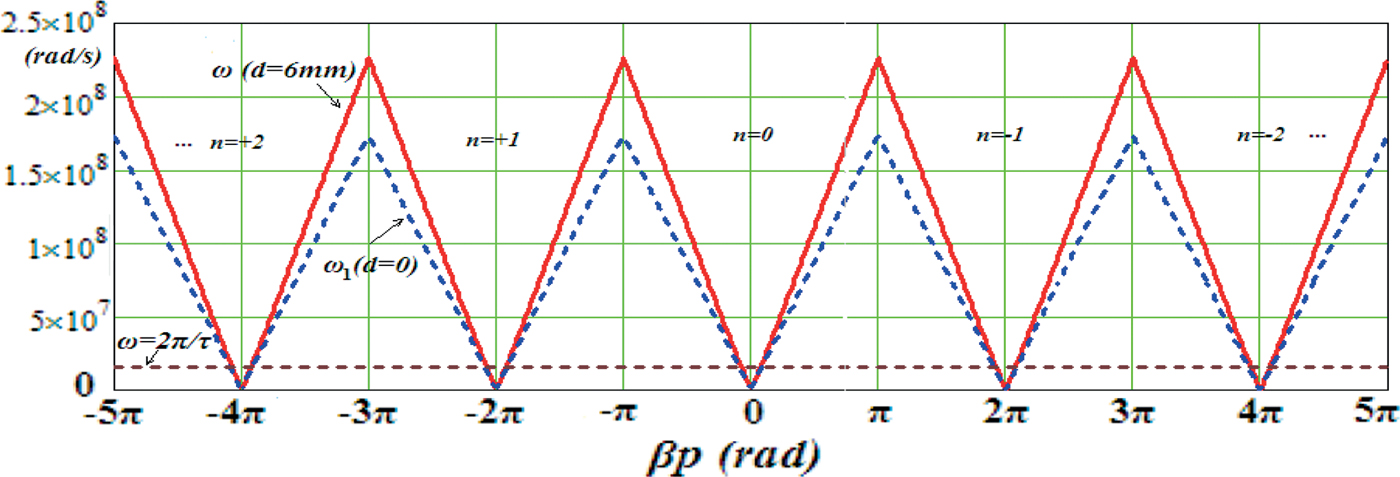
The periodical helical Blumlein type slow-wave system has periodical dispersion curve. Eq. (9) shows the dispersion relation in the first Brillouin zone when –π < β0p < π. By periodical displacements of the abscissa β0p, Eq. (10) presents the dispersion relation ω ~ βp of all the spatial harmonics as Figure 3 shows. When -π < β0p < π, the dispersion curve of the zero harmonic consists of two symmetric lines that pass through the cross point of the coordinates. When the abscissa βp reaches ±π, ω reaches its upper limit 2.263 × 10⁸ rad/s. So, the pass frequency band of the designed helical Blumlein PFL is about (0, 36 MHz). When (2n-1)π < βp < (2n + 1)π, the dispersion curve in Figure 3 corresponds to the n th spatial harmonic, which has the same geometric characteristics as which of the zero harmonic.

Fig. 3. (Color online) Effects of nylon support on the dispersion relation of the spatial harmonics in the slow-wave system.
In order to analyze the effect of the dielectric discontinuity on the dispersion relation, the dispersion curve ω1 ~ βp when d = 0 is also presented in Figure 3 for comparison. Geometric structure of the curve ω1~βp is almost the same as ω ~ βp. However, the slope of curve ω1 ~ βp is smaller than which of the curve ω ~ βp. Pass band of the helical Blumlein PFL with no support dielectric (d = 0) is about (0, 27.6 MHz). So, the conclusion is that dielectric discontinuity increases the frequency of the electromagnetic wave, and the pass band of the helical Blumlein PFL with dielectric discontinuity was also increased by a large extent. The effect of the dielectric discontinuity on dispersion relation of the helical Blumlein PFL is too obvious to be neglected.
For a 400 ns range PFL, the work band of ω is about (0 × 5π × 106 rad/s). The upper limit of the work band 2π/τ = 5π × 106rad/s is plotted in Figure 3 for comparison. Obviously, 2π/τ is much less than the upper limit (36 MHz) of pass band of the PFL with 6 mm-thickness nylon support. As curve ω = 2π/τ intersects with the dispersion curve ω ~ βp in every Brillouin zone, these spatial harmonics may contribute to the electromagnetic field in the PFL. However, the contributions of these harmonics are different from one another. Field coefficient G 1n in Eq. (6) can be selected as spatial harmonic coefficient to measure the proportion of the n th harmonic in the electromagnetic field. By normalizing G 1n to G 10 (coefficient of the zero harmonic), the normalized coefficient of the n th harmonic is defined as k e(n) = G1n/ G10. Especially, k e(0) = 1 corresponds to the zero harmonic. By comparison of these normalized coefficients of spatial harmonics, we can select out the largest ones for analysis.
Actually, through calculating the normalized coefficient k e(n), |k e(n)| < 5 × 10⁻⁴ << k e(0) = 1 when n ≠ 0 in the work band of the PFL. It shows that the electromagnetic wave almost only consists of the zero harmonic. So the conclusion is that, the dispersion characteristics of the PFL are almost determined by the zero harmonic in the first Brillouin zone.
Figure 4 shows the phase velocities of spatial harmonics in the tape helix slow-wave system when d = 0 and d = 6 mm, respectively. The phase velocities of the zero harmonic almost keep constant when abscissa βp increases in the first Brillouin Zone (-π < βp < π). The phase velocities of the higher order harmonic are far smaller than which of the zero harmonic. In the first Brillouin zone, phase velocity of the helical Blumlein PFL with 6 mm-thickness nylon support is much larger than the situation when there is no support dielectric (d = 0). When the 6 mm-thickness nylon support is added to the system, phase velocity of the zero harmonic increases from 5.796 × 10⁶ m/s to 7.573 × 10⁶ m/s (βp = π).

Fig. 4. (Color online) Effects of nylon support on the phase velocity of the spatial harmonics in the slow-wave system
So the conclusions are as follows. (1) When the support dielectric with smaller permittivity (ɛ r2 < ɛr1) is introduced to the tape helix slow-wave system, the angular frequencies and phase velocities of spatial harmonics become much larger than the situation without a support, the “slow” wave effect of the system is weakened, and the electric length of the system is cut down. (2) When ɛr2 > ɛr1, the angular frequencies and phase velocities decrease, the “slow” wave effect of the system is strengthened, and the electric length of the system increases.
4.2. Effects of Dielectric Discontinuity on the Zero Harmonic
As the dispersion characteristics of the designed tape helix slow-wave system are completely determined by zero harmonic at the low frequency band in the first “Brillouin zone,” the dispersion characteristics of the zero harmonic should be analyzed in detail. In order to describe the dispersion characteristics of the zero harmonic in the first “Brillouin zone” more conveniently, ω~γ0 coordinates are employed. By use of Eq. (9) and the parameters in Table 1, the dispersion curves of the zero harmonic are shown in Figure 5 when d ranges from 0 to 6 mm. All of the ω~γ0 curves pass through the cross point of the coordinates. Obviously, when d increases, the angular frequency ω and the slope of ω~γ0 curves also increase. It proves that the dispersion characteristics of the zero harmonic are sensitive to the thickness of nylon support. When f < 10 MHz (ω < 62.8 MHz), γ0 ranges form −10–10 in Figure 5. And this low frequency band just corresponds to the work band of the square pulse accelerator (100 ns range) based on tape helix slow-wave system.

Fig. 5. (Color online) Dispersion curves of the zero spatial harmonic when the thickness of the nylon supports changes.
Figure 6 shows the v ph0~γ0 curves of the zero harmonic in the slow-wave system with de-ionized water as filling dielectric. In Figure 6a, v ph0 is almost a constant at the low frequency band when γ0 changes. That is to say, the intrinsic dispersion of the system determines that v ph0 keeps constant to ω and β0 at low frequency band, which corresponds to good dispersion characteristics. However, when d changes form 0 to 6 mm, v ph0 changes from 5.8 × 10⁶ m/s to 7.08 × 10⁶ m/s. Large increment of v ph0 shows that v ph0 and dispersion characteristics of the zero harmonic are both sensitive to the thickness of nylon support. The conclusion is that support dielectric with larger thickness weaken the “slow” wave effect of the system more effectively.

Fig. 6. (Color online) Effects of support dielectric on the phase velocity of the zero spatial harmonic in the slow-wave system. (a) v ph0vs. γ0 when the thickness of the nylon support changes. (b) v ph0vs. γ0 when the factor g changes (d=6 mm).
In the designed tape helix slow-wave system with 6 mm thickness support, if the relative permittivity ɛr2 of support dielectric changes, then factor g in Eq. (11) also changes, so that phase velocity of the zero harmonic changes. Figure 6b shows the v ph0~γ0 curves when ɛr2 = 1, 2.33, 4.5, 40, 81.5, and 100 (or g = 80, 35, 18, 2, 1, and 0.8). Although v ph0 still almost keeps constant to γ0, it is sensitive to ɛr2 (or the support dielectric categories). When ɛr2 < ɛr1 = 81.5, v ph0 is far larger than the situation without a support dielectric, and smaller ɛr2 corresponds to larger v ph0. On the other hand, v ph0 is smaller than the situation without a support dielectric when ɛr2 > ɛr1 = 81.5. So, the conclusion is that when the permittivity of support dielectric is smaller than that of the filling dielectric, phase velocity of the system is raised, and the “slow” wave effect is weakened. The reverse condition also corresponds to the reverse results.
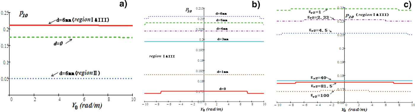
Because the light speed c i is different in different dielectrics, the slow-wave coefficient p l0 (k l0 = v ph0/c i) of the zero harmonic is also different in the three specified regions of the system. Figure 7a shows the p l0~γ0 curves in different regions when the thickness of nylon support is 6 mm. p l0 also keeps constant to γ0 at low frequency band, which proves the dispersion has few effects on p l0. In the de-ionized water (region I and III), p l0 = 0.215; in nylon support (region II), p l0 = 0.05; and when there is no support dielectric (d = 0), p l0 = 0.174. Figure 7b shows the effects of dielectric thickness of nylon on p l0. Obviously, p l0 in region I and III increases from 0.174 (d = 0) to 0.211(d = 6 mm) when d increases from 0 to 6 mm. The “slow” wave effect can be weakened by a large extent, though the increment of d is only 6 mm. If the category of support dielectric changes, p l0 also changes obviously as shown in Figure 7c. When ɛr2 = 1, 2.33, 4.5, 40, 81.5, and 100, p l0 in region I and III decreases from 0.229 to 0.169. It proves that when ɛr2 > ɛr1 = 81.5, the “slow” wave effect of the tape helix system can be strengthened.

Fig. 7. (Color online) Effects of the support dielectric on the slow-wave coefficient p l0 of the zero harmonic. (a) k l0 in different regions of the slow-wave system when the thickness of nylon support d = 6 mm. (b) k l0 in regions I and III when the thickness of the nylon support changes. (c) k l0 in regions I and III when the support dielectric changes (d = 6 mm).
According to Eq. (11), the electric length of the zero harmonic in the system is shown in Figure 8 when d changes. In the low frequency band, electric length τ′0 that also describes the dispersion of the zero harmonic almost keeps the same when γ0 increases. It proves that the intrinsic dispersion of the zero harmonic has few effects on τ′0. However, the thickness of nylon support d does this job. τ′0 decreases from 240 ns to about 198 ns when d increases from 0 to 6 mm. When d = 6 mm, 3 mm and 0, τ′0 = 198 ns, 211 ns, and 240 ns, respectively. For the HPLF (several hundred ns range) based on the tape helix slow-wave system, its pulse duration τ 0 = 2 τ′0. Then τ 0 = 396 ns, 422 ns, and 480 ns when d = 6 mm, 3 mm and 0, respectively. So the conclusion is that, nylon support in the tape helix system with filling dielectric as de-ionized water can bring in a similar “pulse shortening” effect to the HPLF.

Fig. 8. (Color online) Electric length of the slow wave system based on the zero spatial harmonic when d changes.
5. ELECTROMAGNETIC SIMULATION AND EXPERIMENT
5.1. Electromagnetic Wave Simulation
Codes of CST microwave studio suite can be employed to simulate the electromagnetic waves traveling in the tape helix slow-wave system. According to the geometric structure in Figure 1 and parameters in Table 1, electromagnetic wave simulation model was set up as shown in Figure 9a to simulate voltage waves transmitting along the tape helix system. In order to calculate the electric lengths of the voltage waves in regions I and II (r 1 < r < r 2) and in region III (r 2 < r < r 3) simultaneously, port 1 (r 2 < r < r 3, z = 0) and port 2 (r 1 < r < r 2, z = 0) were set on one side of the tape helix system as two voltage input ports as shown in Figure 9a. On the other side of the system, port 3 (r 2 < r < r 3, z = l 0) and port 4 (r 1 < r <r 2, z = l 0) were set as two impedance ports to absorb the electric power. A trapezoid excitation voltage signal with rise time and fall time as 20 ns, flat top time as 100 ns and amplitude as 300 kV, was set to ports 1 and 2 to simulate the quasi-square pulse voltage wave. The time when the front edge of the excitation signal began was set as 0. The impedances of ports 3 and 4 were both set as 16 Ω. The relative permittivity of filling dielectric in the system (de-ionized water, r 1 < r <a, r 2 < r <r 3) is 81.5, and the nylon support thickness d was adjustable. The loss of conductors and dielectrics were neglected, for the PFL was short.

Fig. 9. (Color online) Microwave simulation model and its results of electric lengths. (a) Geometric model. (b) Output voltage signal of the two impedance ports.
The electromagnetic waves excited by the voltage source in ports 1 and 2 transmitted through the tape helix system to ports 3 and 4, and then were absorbed completely if the impedances were matched. By calculating the intervals between the source voltage signal in ports 1 and 2 and output voltage signals in ports 3 and 4, the electric lengths of the pulse voltage waves in regions I and II and region III can be obtained. Electric length is the crucial parameter which expresses the phase velocity and dispersion characteristics of the slow-wave system. So the theoretical analyses in this paper can be demonstrated by the demonstration of electric length.
In simulation, the thickness d of nylon support was set as 6 mm and 3 mm orderly, and the simulation results are shown in Figure 9b. Curve 1 represents the excitation voltage signal in ports 1 and 2, curves 2 and 3, represent the output voltage signals in ports 3 and 4 respectively, when d = 6 mm. Through the comparison with curve 1, the times when the flat top started in curves 2 and 3 were about 180 ns and 190 ns later than the counterpart in curve 1, respectively. That is to say, the electric lengths of the system were about 180 ns and 190 ns in region III and region I and II, respectively. These results basically corresponded to the theoretical result 198 ns in Figure 8. When d = 3 mm, the electric lengths of the system were about 200 ns and 215 ns in region III and regions I and II, respectively, as shown in curves 4 and 5 in Figure 9b. These two results were also basically corresponded to theoretical result 211 ns in Figure 8.
Simulation results proved that thickness of the nylon support and the dielectric discontinuity does have obvious impacts on the electric length and dispersion characteristics of the tape helix slow-wave system.
5.2. Experiment
In order to testify the theoretical calculation and simulation result of the electric length, which describes the dispersion characteristics of the tape helix slow-wave system at low frequency band, the experimental platform system of a pulse accelerator was set up, and its structure is shown in Figure 10a. The accelerator platform system consisted of a primary capacitor, a trigger, a pulse transformer, a spark gap, tape-helix Blumlein PFL, a dummy load and capacitive voltage dividers. Actually, the tape-helix Blumlein PFL was an electromagnetic wave transmission line based on the tape helix slow-wave system, which was very suitable for tests on electric length.

Fig. 10. (Color online) Experimental platform and results. (a) Experimental platform for the helical Blumlein PFL based on the tape helix slow-wave system. (b) Output voltage pulse signal of the 32 Ω dummy load formed by the tape helix slow-wave system (d = 6 mm). (c) Output voltage and current pulse signals of the 32 Ω dummy load formed by the tape helix slow-wave system (d = 3 mm).
The work principle of the accelerator platform system is as follows. The primary capacitor and pulse transformer with a closed amorphous core charged the tape helix slow-wave system to 10–20 kV, and the charge time was about 10–12 µs. The self-breakdown spark gap with two spherical electrodes broke down when the charge voltage of the PFL reached its breakdown voltage. Then, the tape helix slow-wave system as an electromagnetic wave transmission line discharged to the dummy load through the spark gap, and the formed high-voltage quasi-square pulse voltage signal can be obtained on the dummy load.
In order to study the effects of support dielectric thickness on the electric length of the tape helix slow-wave system, two air-core cylindrical nylon supports with thickness of 6 mm and 3 mm were used in the experiments. When d = 6 mm, the voltage signal of the 32 Ω dummy load in experiment is shown in Figure 10b. The amplitude of the formed voltage pulse was 15 kV, flat top was 180–190 ns, and the pulse width at half maximum was 377 ns. The front edge of the formed pulse was long, due to the parasitic inductance and spark inductance in the platform system. Because the pulse duration of the tape-helix Blumlein PFL is twice as the electric length of the tape helix slow-wave system, the electric length was about 188.5 ns when d = 6 mm. When d = 3 mm, Figure 10c shows the voltage and current pulse signals of the 32 Ω dummy load formed by the tape-helix Blumlein PFL. Waveform of the 0.4 kA current pulse was in line with the 12 kV voltage pulse. The voltage pulse duration was about 400 ns (pulse width at half maximum) in experiment, so the electric length was 200 ns when d = 3 mm. By Fourier transformation, the spectrum of the quasi-square voltage pulses shown in Figures 10b and 10c were in the band f < 3 MHz, which satisfied the low frequency band condition f < 10 MHz adopted in Figures 5 to 8.
When d = 6 mm and 3 mm, theoretical calculation of electric lengths of the tape helix slow-wave system was 198 ns and 211 ns, while the experimental results showed that the electric lengths were 188.5 ns and 200 ns, respectively. The theoretical calculation had relative errors as 5% and 5.5%, respectively.
Generally speaking, according to Eq. (11), the electric length is an important parameter which directly describes phase velocity and the dispersion characteristics (ω~γ0) of the tape helix slow-wave system. The correspondence of experimental result and theoretical calculation of electric length demonstrated that, the dispersion analysis of the effects of dielectric discontinuity on the slow-wave system was correct and reasonable. The nylon support in the tape helix slow-wave system with filling dielectric as de-ionized water did bring in a similar “pulse shortening” effect to the HPLF.
6. CONCLUSIONS
In this work, the tape helix slow-wave system, including an inner and an outer metal shield, tape helix, nylon support, and de-ionized water as filling dielectric, was studied. Effects of radial dielectric discontinuity caused by the support dielectric and filling dielectric on the dispersion characteristics were analyzed in detail for the first time. The dispersion relations, phase velocities, slow-wave coefficients and electric lengths of the spatial harmonics in the system were calculated. Results showed that, if the permittivity of support dielectric was smaller than that of filling dielectric, frequencies of the spatial harmonics in the system rose, phase velocities and slow-wave coefficients increased, the slow-wave effect of the system was weakened so that the previous electric length was shortened. The reverse condition corresponded to the reverse results, and the electromagnetic simulation also proved it. By use of the HPLF platform based on the studied tape helix slow-wave system, the electric lengths of the system were tested as 188.5 ns and 200 ns in experiment, when the thicknesses of nylon support were 6 mm and 3 mm, respectively. The theoretical calculation results 198 ns and 211 ns basically corresponded to experimental results, which only had relative errors as 5% and 5.5%. Experimental results demonstrated the similar “pulse shortening” effect in the tape helix slow-wave system caused by the dielectric discontinuity.
ACKNOWLEDGMENTS
This work was supported by the National Science Foundation of China under Grant No.51177167. It's also supported by the Fund of Innovation, Graduate School of National University of Defense Technology under Grant No. B100702.