
The traditional approach to data analysis in regional dialectology involves three steps (Kurath, Reference Kurath1949; Labov, Ash, & Boberg, Reference Labov, Ash and Boberg2006). First, the values of numerous linguistic variables are analyzed to identify individual patterns of regional linguistic variation. This is accomplished by mapping the values of each variable across a set of locations and then plotting an isogloss—a line that divides a map into regions where the different values of the variable predominate (Chambers & Trudgill, Reference Chambers and Trudgill1998; Kretzschmar, Reference Kretzschmar1992, Reference Kretzschmar2003). For example, Kurath (Reference Kurath1949:Figure 134) mapped three terms for cornhusks on the American East Coast. The map shows that shucks predominates in the Carolinas and much of Virginia; husks predominates in New England, New York, New Jersey, and Pennsylvania; and both forms occur in West Virginia and the Delmarva Peninsula, where caps also occurs. To represent this pattern, Kurath plotted an isogloss separating Pennsylvania from Virginia. As is common in regional dialectology, the isogloss did not represent a limit of occurrence, as there were numerous husk locations on the shuck side of the isogloss and vice versa, but rather the approximate location of the border separating the region where husk predominated from the region where shuck predominated. As is also common, Kurath determined the location of the isogloss based on his own judgment. He analyzed the map and drew a line. Replicable algorithms for plotting isoglosses have been developed (e.g., Labov, Ash, & Boberg, Reference Labov, Ash and Boberg2006), but they are still only formalizations of the judgments of the dialectologists who designed them. Because these methods are not statistically justified, plotting an isogloss does not test if a regional pattern is present. A pattern is assumed to exist, and then an isogloss is plotted.
In the second step of data analysis, linguistic variables that exhibit similar patterns of regional variation are identified by searching for bundles of isoglosses—isoglosses for different variables that follow similar paths (Chambers & Trudgill, Reference Chambers and Trudgill1998). For example, in addition to plotting an isogloss for cornhusks, Kurath (Reference Kurath1949:Figure 30) also plotted isoglosses for wheat bread and the second-person plural pronoun. Based on these maps, Kurath concluded that the isoglosses for all three variables were similar enough to constitute an isogloss bundle, indicating that an important boundary between two dialect regions ran along the southern border of Pennsylvania. Once again, this step is usually based on a simple subjective analysis. A more complex approach to aggregation, called the schematic participation method, was employed by Carver (Reference Carver1987), who classified locations into dialect layers based on the percentage of shared lexical variants. For example, a primary dialect layer might be plotted to demarcate a region containing locations that use 100% of the same variants and a secondary dialect layer might be plotted to demarcate a region containing locations that use 70%–99% of those variants. Carver defined different dialect layers based on different sets of lexical variables, including a layer that split Pennsylvania from Virginia. However, whereas the schematic participation method is a quantitative procedure for aggregating the values of multiple linguistic variables, the crucial step of selecting the variables that define a particular layer is still based on the judgment of the dialectologist.
In the third step of data analysis, dialect regions are identified based on an analysis of the relationship between the various bundles of isoglosses. Once again, this step is usually achieved through a subjective analysis, with the dialectologist identifying dialect regions based on how the various isogloss bundles section the map into subregions. For example, based on the isogloss bundles for dozens of lexical variables, Kurath (Reference Kurath1949:Figure 3) split the eastern United States into three primary dialect regions: the North, the Midland, and the South. This three-way division on the East Coast has since become the standard mapping in American dialectology (see Wolfram & Schilling-Estes, Reference Wolfram and Schilling-Estes2006) and has recently been replicated by Labov, Ash, and Boberg (Reference Labov, Ash and Boberg2006) based on an analysis of phonetics and phonology. Carver (Reference Carver1987), however, identified only two major regions on the American East Coast: the North and the South. The number of dialect regions on the East Coast of the United States is perhaps the biggest debate in American dialectology (e.g., see Davis & Houck, Reference Davis and Houck1992); however, it is difficult to choose between these competing theories because these theories have been based on the subjective analysis of linguistic data.
Whereas American dialect studies are traditionally based on subjective analyses, a quantitative approach to the analysis of regional linguistic variation has been developed in the largely European approach to dialectology known as dialectometry (Goebl, Reference Goebl1982, Reference Goebl1984, Reference Goebl2006; Heeringa, Reference Heeringa2004; Nerbonne, Reference Nerbonne2006; Nerbonne & Kleiweg, Reference Nerbonne and Kleiweg2003, Reference Nerbonne and Kleiweg2007; Nerbonne & Kretzschmar, Reference Nerbonne and Kretschmar2003, Reference Nerbonne and Kretschmar2006; Séguy Reference Séguy1971, Reference Séguy1973a, Reference Séguy1973b). There are two primary advantages to a statistical approach. First, a statistical approach allows patterns to be identified objectively, unbiased by the assumptions of the dialectologist. Adopting a statistical approach not only avoids the identification of spurious regional patterns, but it also allows for the identification of regional patterns that may have gone unnoticed in a traditional analysis. Second, a statistical approach is replicable, allowing analyses to be reproduced and to be conducted consistently across different datasets. However, whereas dialectometry provides a statistical method for the analysis of regional linguistic variation, it does not follow the same steps as a traditional analysis, forgoing the analysis of individual linguistic variables and the identification of subsets of linguistic variables that exhibit similar regional patterns. In standard dialectometry, the first step of data analysis involves calculating the linguistic distance between all pairs of locations in the dataset based on the values of the complete set of variables (although see Rumpf, Pickl, Elspass, Koenig, & Schmidt, 2009, 2010). For example, similar to the schematic participation method, the linguistic distance between two locations is often measured as the percentage of shared vocabulary items or pronunciations. The resultant linguistic distance matrix can then be analyzed using multivariate statistics to identify dialect regions, but because the complete set of variables is aggregated first, it is impossible to identify regional patterns in the values of individual variables or to determine if different subsets of variables exhibit different regional patterns.
The goal of this paper is to present a statistical approach to the analysis of regional linguistic variation that is based on the same series of steps as a traditional analysis. The traditional approach identifies regional linguistic variation in a straightforward and logical manner, but this approach has never been implemented using statistical methods. This paper shows how these same basic goals can be achieved through a quantitative analysis based on a combination of three statistical techniques: spatial autocorrelation, factor analysis, and cluster analysis. To introduce this method and illustrate its application, this paper presents an analysis of regional lexical variation in written English, based on the values of 40 lexical alternation variables in a 26-million-word corpus of letters to the editor representing 206 cities from across the United States. Before describing the method in detail and presenting the results of the analysis, the corpus and the lexical variables are introduced.
CORPUS COMPILATION
The corpus analyzed in this study consists of 26 million words representing the letter to the editor register as written in 206 cities from across the United States. The corpus was originally compiled to analyze regional linguistic variation in written American English (Grieve, Reference Grieve2009). Although dialect surveys are usually based on data gathered through linguistic interviews (although see, e.g., Inhalainen, Reference Ihalainen and Thomas1988, Reference Ihalainen, Aarts and Meijs W1990, Reference Inhalainen, Aijmer and Altenberg1991; Kortmann, Herrmann, Pietsch, & Wagner, Reference Kortmann, Herrmann, Pietsch and Wagner2005; Szmrecsanyi, Reference Szmrecsanyi2008), a corpus-based approach was adopted because it greatly facilitated the collection of large amounts of written data from informants from across the United States.
The letter to the editor register was selected for analysis for numerous reasons. First, it was necessary to select a variety of language that allowed for geographical information about the informants to be retrieved. The place of residence of an author of a letter to the editor is usually identified in the byline. Second, it was necessary to select a variety of language that is produced by a large number of people from across the United States. Letters to the editor are published daily in newspapers from cities and towns in every state. Furthermore, many newspapers make archives of letters to the editor available online, allowing the data to be collected with ease. Finally, letters to the editor were selected because focusing on this variety of language allows for register and temporal linguistic variation to be controlled. Register variation is limited because the letter to the editor is a common, specific, and highly conventionalized register, which ensures that the vast majority of letters in the corpus are written in a very consistent form with very similar communicative purposes. Temporal linguistic variation is limited because letters to the editor are published very frequently, which allows a large corpus to be compiled that spans a relatively short period. Controlling for both of these factors is standard practice in traditional dialect surveys, where data is collected over a limited number of years through carefully conducted interviews.
Unlike traditional dialect surveys, however, analyzing letters to the editor does not allow for length of residence to be controlled. In the final corpus, informants were classified as representing the city in which they currently live, as listed in the byline of the letter, regardless of how long they have lived at that location. Although focusing on the language of lifelong residents has facilitated the identification of regional linguistic variation in traditional dialect studies, controlling for length of residence is not a requirement for a dialect study. In fact, to analyze synchronic regional linguistic variation, the language of both short- and long-term residents must be available for analysis, as both are members of the speech community at that specific point in time. To identify current and pervasive patterns of regional linguistic variation, it is necessary to analyze the language of the entire population, not just a sample of the population that represents a historical speech community. It would be ideal to know the length of residence of every informant so that the significance of this factor could be analyzed directly. However, not knowing this information does not invalidate the dataset, just as it does not invalidate datasets used in geographic analyses of demographic, economic, and political patterns, where length of residence is almost never controlled by default.
In addition, analyzing letters to the editor does not allow for the demographic background of informants to be controlled. Aside from gender, which can usually be inferred from the name of an informant, the age, race, and socioeconomic status of letter writers are usually unknown. The gender of the informants in the final corpus was not found to exhibit a significant regional pattern, based on an analysis of global spatial autocorrelation as introduced in this paper. This is not surprising, given the fact that gender does not exhibit much regional variation across the United States; however, it is almost certain that other social variables are regionally patterned in the final corpus. For example, there is a higher percentage of Hispanic people in the Southwest, and therefore there is presumably a higher percentage of Hispanic letter writers in Southwestern newspapers. Though such regional demographic patterns will undoubtedly affect regional linguistic variation, the demographic background of informants does not need to be kept stable across locations in a dialect study (e.g., see Labov, Ash, & Boberg, Reference Labov, Ash and Boberg2006) because demographic background is a property of the speech communities under analysis. Furthermore, in the final corpus analyzed here, the demographic background of the informants from each city is representative of the demographic background of the population that participates in that register in that city, because letters were almost always sampled exhaustively from a newspaper over a given period. Again, it would be ideal to have access to more social information, but it is not necessary to know the demographic background of every informant to conduct a principled analysis of regional linguistic variation.
It is also important to note that even though letters to the editor can be edited by newspaper staff, it does not appear that editing will confound the results of an analysis of regional linguistic variation in this register. Based on discussions conducted through email with editorial pages editors from various newspapers represented in the corpus, it is clear that letters to the editor are edited to a certain degree, but mainly for length. Although it is relatively common for passages to be deleted from long letters by the editorial staff of a newspaper, given a large enough corpus, such deletions should have no affect on the values of linguistic alternation variables. Letters are also edited for grammatical, typographical, punctuation, and content errors, but according to the editorial page editors, grammatically correct sentences are rarely altered. Indeed, reading over letters to the editor, it is clear that letters with grammatical errors are published frequently, offering further evidence that editing is relatively limited. For these reasons, it is assumed that editing will not confound the analysis of many linguistic variables—including those variables under analysis in this study, which mostly involve the alternation between function words that are both acceptable in written Standard American English.
The corpus was compiled by downloading letters to the editor published by major newspapers from across the contiguous United States. The 206 cities represented in the corpus, which are mapped in Figure 1, were selected to include most of the major cities in the United States, while also representing the major subregions within each state. According to the 2000 census, the top 30 metropolitan areas in the United States are represented in the corpus and the top 50 metropolitan areas are represented in the corpus except for Providence, Rhode Island, and Birmingham, Alabama. These cities were excluded because suitable archives were not available for the major newspapers in these cities, although smaller cities nearby were sampled in their place. In addition, smaller cities and towns were also sampled to fill in other regional gaps in the corpus. As is clear in Figure 1, however, the distribution of the cities in the corpus is not entirely even. Sampling is denser in the Northeast and sparser in the North Central States, reflecting general patterns of population density. The result of this uneven distribution is that dialect patterns can be identified with greater confidence and resolution in regions with better coverage. In each city, only major daily newspapers were targeted for download. In those few cities where more than one major newspaper exists, letters were taken from all of the major newspapers for which suitable archives were available. Whenever possible, letters from the years 2005–2008 were targeted for download; however, when necessary, letters from 2000–2010 were sampled in order to increase the size of the corpus.

Figure 1. City Subcorpora.
Once downloaded, each letter was sorted into a city subcorpus based on its author's current place of residence.Footnote 1 To maximize the size of the corpus, most letters were sorted into core-based statistical areas (CBSA). The U.S. Census Bureau uses CBSA to denote a region consisting of a county containing a core urban area with a population of at least 10,000 people and any adjacent counties with a high degree of socioeconomic integration—essentially a city and its suburbs. Letters were sorted by CBSA rather than by municipality to increase the size of the corpus by allowing letters from the area surrounding a city to be included in the corpus. However, in order to increase the number of city subcorpora, whenever a sufficient number of letters were available, letters were sorted by metropolitan division—one or more counties that constitute a distinct employment region within a CBSA. For example, city subcorpora were formed for both San Francisco and Oakland because a sufficient number of letters were downloaded from each of these metropolitan divisions. In addition, one subcorpus was compiled containing letters written by the residents of Brattleboro, Vermont, even though this municipality is not a part of any CBSA (due to its isolation and small population), because a sufficient number of words were obtained from this town.
After the letters were sorted into city subcorpora, each city subcorpus containing at least 35,000 words was retained for analysis. A 35,000 word cutoff was selected because this gave a sufficient number of words in a city subcorpus to obtain reasonable estimates of the values of the 40 function word alternation variables under analysis (i.e., at least 10 total tokens of each variable on average per city subcorpus). Although there is a great deal of variation in the size of the individual city subcorpora (from 37,228 words for Aberdeen, South Dakota, to 317,592 words for Nashville, Tennessee), each of the variables is measured as a proportion, and as such, the values of the variables are normalized. Assuming that the token frequency for each variable is sufficient in each corpus, the variation in the size of the subcorpora is largely irrelevant. In total, the final corpus contains 26,573,826 words, spread across 159,181 letters, written by 130,659 authors, representing 206 cities from across the contiguous United States (see Figure 1).
CORPUS ANALYSIS
As in variationist sociolinguistics, dialect studies often focus on linguistic alternation variables, which consist of a set of variant linguistic forms that have the same meaning (Chambers & Trudgill, Reference Chambers and Trudgill1998; Geeraerts, Grondelaers, & Bakema, Reference Geeraerts, Grondelaers and Bakema1994; Labov, Reference Labov1966a, Reference Labov1966b, Reference Labov1972; Wolfram, Reference Wolfram1969, Reference Wolfram1991). In regional dialectology, the linguistic alternation variables most often analyzed consist of sets of equivalent pronunciations or synonymous words. Alternation variables are also usually measured categorically, where each informant or location is associated with just of one of the variants of the variable. However, as is common in variationist sociolinguistics, alternation variables can also be measured continuously in dialectology (e.g., Bloch, Reference Bloch, Allen and Underwood1971), where each informant or location is associated with a quantitative value representing the frequency of one of the variants of the variable relative to all of the variants of the variable in a discourse sample. Modern dialect surveys (Labov, Ash, & Boberg, Reference Labov, Ash and Boberg2006) have also analyzed the values of acoustic variables, especially vowel formant variables, which are also measured quantitatively but do not involve alternations. The basic method being introduced here can be used to analyze any of these types of linguistic variables, but in this paper, the method is used specifically to analyze the values of 40 continuously measured lexical alternation variables.
To compute the value of an alternation variable with two variants in a city subcorpus, the proportion of one variant was measured by dividing the total tokens of that variant (V a) in the subcorpus by the total tokens of the variable in the subcorpus: that is, the total number of tokens of both the first (V a) and the second (V b) variant (Equation 1). It does not matter relative to which of the two variants the proportion is measured.
This formula is the basis of all of the function word alternation variables analyzed in this study, where, in the simplest cases, the proportion of one word is measured relative to one other synonymous word.
High-frequency lexical alternations, primarily function word alternations, were chosen for analysis because they are some of the few alternation variables that are sufficiently frequent and variable in letters to the editor to warrant analysis. It was, however, difficult to compile a list of function word alternations for analysis, as alternation variables are not usually analyzed in written English. Most nonphonological alternation variables that have been analyzed in dialectology and sociolinguistics (e.g., double negation, agreement error, content word alternations) are not suitable for analysis in letters to the editor because they are insufficiently frequent and/or variable in written English, as they often involve a highly nonstandard variant, which almost never occurs in published written English. As such, it was necessary to compile a list of suitable lexical alternation variables by hand. This was accomplished by looking through lists of high frequency function words and adverbs and then manually identifying words that have the same or nearly the same meaning in at least certain contexts. In addition, selections of the letters to the editor were read in order to identify common function word alternations in this register, which is a standard method for the identification of variables in sociolinguistic research (Wolfram, Reference Wolfram and Preston1993).
The 40 linguistic variables analyzed in this study are introduced in Table 1, which is organized by part-of-speech and which lists the two variants under analysis. Although most of the variants are vocabulary items that are equivalent or nearly equivalent in almost every case, a few variables involve alternations that are only equivalent in certain environments (such as pairs of prepositions that only alternate following certain nouns). The contexts in which these pairs of variants were counted are described in the final column of the table. Although none of the variables can be measured with perfect accuracy, the algorithms used to count these variables were each tested on hundreds of sentences drawn at random from the corpus, and in all cases, the algorithms were found to correctly identify tokens of the variables over 90% of the time and usually over 95% of the time. Furthermore, one of the advantages of the method being introduced here is that regional patterns can be identified in the presence of noise, such as variation in the value of a linguistic variable caused by minor inaccuracies in the algorithms used to count these variables.
Table 1. Lexical alternation variables

aIf and whether were only counted following forms of the following verbs: wonder, care, question, determine, see, consider, ask, know, debate, tell, and decide.
bAbout and on were only counted following forms of the following nouns: research, comment, article, impact, letter, report, information, story, debate, opinion, column, view, editorial, and book.
cTo and toward(s) were only counted following forms of the following nouns: contribution, gratitude, threat, respect, responsibility, commitment, devotion, donation, and courtesy.
Finally, before conducting a statistical analysis, the raw values of the 40 lexical variables were mapped individually across the cities represented in the corpus. The maps for anyone/anybody alternation and though/although alternation are presented in Figures 2 and 3.Footnote 2 Upon close inspection, regional patterns can be discerned in many of these maps, such as the relative frequency of anybody in the West and of although in the Northeast. In every case, however, the patterns are far from absolute, and their statistical significance is thus unclear.

Figure 2. Anyone/anybody alternation.

Figure 3. Though/although alternation.
STATISTICAL ANALYSIS
The statistical approach to the analysis of regional linguistic variation being introduced in this paper consists of three steps, which correspond to the three basic steps of a traditional analysis of regional linguistic variation. First, the individual linguistic variables are subjected to an analysis of spatial autocorrelation to identify significant patterns of regional linguistic variation, which is similar to plotting isoglosses. Second, the results of the spatial autocorrelation analysis are subjected to a factor analysis to identify common patterns of regional linguistic variation, which is similar to identifying bundles of isoglosses. Third, the results of the factor analysis are subjected to a cluster analysis to identify dialect regions, which is similar to identifying dialect regions based on how bundles of isoglosses divide a region into subregions. To demonstrate the application of the method, it was used to analyze regional linguistic variation in the dataset described, which consists of the values of 40 lexical alternation variables measured across 206 American cities.Footnote 3
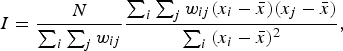
Spatial autocorrelation analysis
To identify significant patterns of regional variation in the values of the 40 individual linguistic variables, each variable was tested independently for patterns of global and local spatial autocorrelation. Spatial autocorrelation is a measure of spatial dependency that allows for the degree of spatial clustering in the values of a variable measured across a series of locations to be gauged (Cliff & Ord, Reference Cliff and Ord1973, Reference Cliff and Ord1981). To test if the values of a variable exhibit an overall pattern of spatial clustering, global spatial autocorrelation was analyzed using global Moran's I (Moran, Reference Moran1948; Odland, Reference Odland1988). To identify the location of high- and low-value clusters in the distribution of an individual variable, local spatial autocorrelation was analyzed using local Getis-Ord Gi* (Ord & Getis, Reference Ord and Getis1995). Although basic global spatial autocorrelation statistics were introduced to regional dialectology in Lee and Kretzschmar (Reference Lee and Kretzschmar1993) and Kretzschmar (Reference Kretzschmar1996), measures of spatial autocorrelation have not been used in regional dialectology since, despite their obvious application and their frequent use in other fields.
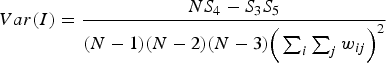
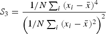
Global Moran's I (Moran, Reference Moran1948; Odland, Reference Odland1988) was used to test each linguistic variable for significant levels of positive global spatial autocorrelation to determine if each variable exhibits an overall pattern of regional clustering. The value of Moran's I usually ranges from –1 to +1, where a significant negative value indicates that nearby locations tend to have different values, a nonsignificant value approaching 0 indicates that nearby locations tend to have random values, and a significant positive value indicates that nearby locations tend to have similar values (Odland, Reference Odland1988). The formula for calculating global Moran's I is provided in Equation 2 (Odland, Reference Odland1988).
where N is the total number of locations, x i is value of the variable at location i, x j is value of the variable at location j, ![]() is the mean for the variable across all locations, and w ij is the value of the spatial weighting function for the comparison of locations i and j.
is the mean for the variable across all locations, and w ij is the value of the spatial weighting function for the comparison of locations i and j.
The spatial weighting function is a set of rules that assigns a weight (w ij) to the comparison of every pair of locations in the distribution of a variable so that comparisons between locations that are close together are given greater weight than comparisons between locations that are far apart (Odland, Reference Odland1988).Footnote 4 The simplest and most common spatial weighting function is a binary weighting function, which assigns a weight of 1 to all pairs of locations within a certain distance and a weight of 0 to all other pairs of locations (Odland, Reference Odland1988). The cutoff distance essentially sets the level of resolution for the analysis. A smaller cutoff is better for identifying smaller clusters, whereas a larger cutoff is better for identifying larger clusters. Setting the cutoff distance is problematic, however, because it is possible for different linguistic variables to exhibit regional patterns at different levels of resolution. To identify spatial clustering in the values of individual variables as accurately as possible, it is important to fit the spatial weighting function for each variable. This was accomplished by calculating global Moran's I for each variable for a range of different cutoffs and by then selecting the cutoff that identified the most significant spatial clustering for that variable.
To interpret the significance of Moran's I, a standardized z-score was obtained under the assumption of randomization (Odland, Reference Odland1988).Footnote 5 Because numerous linguistic variables were being analyzed for regional patterns, the level of statistical significance was adjusted using a Bonferroni correction to correct for multiple comparisons. A variable was deemed to exhibit significant global autocorrelation if the computed z-score was larger than or equal to 3.02, corresponding to a one-tail .00125 significance level, which was selected based on a Bonferroni correction for 40 variables (.05/40 = .00125). A Bonferroni correction controls for the fact that every time a variable is added to the analysis, the likelihood that a significant pattern will be found by chance increases. A one-tail test of significance (Odland, Reference Odland1988) was used instead of a two-tail test because the goal of the analysis was to detect spatial clustering by testing for positive global autocorrelation. As opposed to other quantitative methods used to analyze regional patterns in the values of individual linguistic variables (e.g., Rumpf et al., Reference Rumpf, Pickl, Elspass, Koenig and Schmidt2009, Reference Rumpf, Pickl, Elspass, Koenig and Schmidt2010), one of the major advantages of Moran's I is that it allows for statistically significant regional patterns to be identified.
Based on this adjusted significance level, five variables were found to exhibit significant positive spatial autocorrelation using a 500-mile binary spatial weighting function, indicating that some variables exhibit significant regional clustering when analyzed using an arbitrary spatial weighting function. Similar results were obtained for a range of arbitrary cutoff distances, although different subsets of variables were found to exhibit significant autocorrelation at different cutoffs, justifying the use of fitted spatial weighting functions. The results of the final global autocorrelation analysis using the fitted spatial weighting functions are presented in Table 2, which lists the mean value, the cutoff distance for the spatial weighting function, Moran's I, the corresponding z-score, and the one-tailed p value (significant at .00125) for each variable. Using the fitted spatial weighting functions, 10 variables were found to exhibit significant levels of positive global spatial autocorrelation, including anyone/anybody alternation (Figure 2) and though/although alternation (Figure 3).
Table 2. Global spatial autocorrelation results

In addition to measuring global spatial autocorrelation, which tests whether the values of a variable exhibit significant spatial clustering, local spatial autocorrelation was measured to identify the location of high- and low-value clusters. Unlike a measure of global spatial autocorrelation, which returns one value for a variable indicating the degree of clustering across the entire distribution of that variable, a measure of local spatial autocorrelation returns one value for each location for a variable indicating the degree to which that particular location is part of a high- or low-value cluster. The results of the local spatial autocorrelation analysis can then be mapped to identify the specific locations of high- and low-value clusters for each variable, which may not have been obvious based on an analysis of the raw values of the variable. This procedure is essentially a quantitative analog to the identification of isoglosses in traditional dialectology.
To measure local spatial autocorrelation, local Getis-Ord Gi* (Ord & Getis, Reference Ord and Getis1995) was calculated for each location for each variable using Equations 3 and 4.
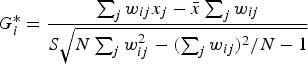
Local Getis-Ord Gi* returns a z-score indicating the degree to which a location is surrounded by locations with similar values. A significant negative Getis-Ord Gi* z-score indicates that the location is part of a low-value cluster, whereas a significant positive Getis-Ord Gi* z-score indicates that the location is part of a high-value cluster. A Getis-Ord Gi* z-score was interpreted as significant if it was larger than or equal to ±3.23 because this z-score corresponds to a two-tail .00125 alpha level, which was selected based on a Bonferroni correction of the standard .05 alpha level for 40 variables (.05/40 = .00125). A two-tail test of significance was used instead of a one-tail test because the goal of the analysis was to identify both high- and low-value clusters.
By plotting the Getis-Ord Gi* z-scores, it is possible to identify the location of spatial clusters in the values of a variable. For example, local spatial autocorrelation maps for anyone/anybody alternation and though/although alternation are presented in Figures 4 and 5. In these maps, a positive z-score (i.e., light shades) indicates that the first variant occurs relatively frequently in that region, whereas a highly negative z-score (i.e., dark shades) indicates that the second variant occurs relatively frequently in that region. Figure 4 shows that anyone is relatively common in the Midwest and the South, whereas anybody is relatively common in the West. Figure 5 shows that although is relatively common in the Northeast, whereas though is relatively common in the South Central states. By comparing the raw maps to the corresponding autocorrelation maps it is possible to see how the Getis-Ord Gi* analysis identifies underlying regional signals in the values of a linguistic variable. It should also be noted that whereas the global autocorrelation analysis only identified 10 variables that exhibit significant global patterns, due primarily to the conservativeness of the Bonferroni correction, the local autocorrelation analysis identified clear patterns in many other variables.

Figure 4. Anyone/anybody local autocorrelation.

Figure 5. Though/although local autocorrelation.
Factor analysis
To identify common patterns of regional linguistic variation, the results of the local spatial autocorrelation analysis were subjected to a factor analysis. A factor analysis is a multivariate statistic that identifies common patterns of variation in a set of variables measured over a large number of observation points, by generating a series of factors that represent a common pattern of variation in the set of variables (Hair, Black, Babin, Anderson & Tatham, Reference Hair, Black, Babin, Anderson and Tatham2006; Tabachnick & Fidell, Reference Tabachnick and Fidell2007). Because the local Getis-Ord Gi* z-scores computed in the previous stage of the analysis represent the location of spatial clusters in the values of the individual linguistic variables, subjecting this dataset to a factor analysis identifies common patterns of spatial clustering.Footnote 6 By plotting the factor scores, it is possible to map these common patterns of regional linguistic variation. This procedure is essentially a quantitative analog to the identification of isogloss bundles in traditional dialectology.
A factor analysis was used to analyze the Getis-Ord Gi* z-scores rather than the raw values of the linguistic variables (cf. Labov, Ash & Boberg, Reference Labov, Ash and Boberg2006; Nerbonne, Reference Nerbonne2006; Shackleton, Reference Shackleton2005) in order to focus the analysis on regional linguistic variation. If the raw values were subjected to a factor analysis, many patterns of spatial clustering that were identified by the analysis of local spatial autocorrelation would be lost. As such, it is necessary to apply the local spatial autocorrelation analysis first to extract the underlying spatial pattern from the values of each variable. The Getis-Ord Gi* z-scores can then be subjected to a factor analysis to identify common patterns of spatial clustering. If the original variables had exhibited clearer regional patterns, then it would not have been necessary to apply the local spatial autocorrelation analysis. However, it would seem that in raw natural language data, linguistic variables are rarely distributed in clear regional patterns (e.g., see Labov, Ash, & Boberg, Reference Labov, Ash and Boberg2006:77–118), presumably because there are many other factors that affect linguistic variation. These factors may be stronger than regional linguistic variation and often are very difficult to control, such as variation in data collection procedures, idiosyncratic variation, temporal variation, register variation, topical variation, and variation in the age, gender, socioeconomic status and ethnicity of informants. By analyzing the smoothed variables generated by the local autocorrelation analysis, it is possible to ignore these other forms of linguistic variation and focus instead on identifying common underlying patterns of regional linguistic variation.
The factor analysis was set to extract three factors using varimax rotation. A three-factor solution was selected because the first three factors accounted for 54% of the variance in the set of 40 variables (with Factor 1 accounting for 24% of the variance, Factor 2 accounting for 18%, and Factor 3 accounting for 12%), whereas adding a fourth factor would have only accounted for an additional 6% of the variance in the dataset. The fact that three factors account for over 50% of the regional variation in a set of 40 variables shows that there are consistent regional patterns in the dataset. Varimax rotation was used to limit the number of factors onto which each variable loads, which causes the factors to more clearly reflect the spatial patterns visible in the local autocorrelation maps of the individual linguistic variables. Varimax rotation is also in line with the goals of a traditional analysis, where variables are usually only indentified as being part of one bundle of isoglosses.Footnote 7
Table 3 lists the variable loadings (larger than or equal to .300) for the three factors, which describe the degree to which the regional pattern exhibited by each of the variables is represented by each of the factors. Despite rotation, a variable can load on more than one factor because different factors can represent different parts of the regional pattern exhibited by a variable, although, in this case, most variables load very strongly on only one factor. The sign of a loading only reveals which variant characterizes the common high- and low-value clusters identified by the factor analysis, which was an arbitrary decision. Table 3 also lists the uniqueness value for each of the variables, where a high value (especially larger than .800) indicates that the pattern exhibited by that variable is not represented well by the complete three-factor solution. In this case, the three-factor solution represents all of the variables well. To identify the regional patterns represented by the three factors, the factor scores were mapped (Figures 6–8).

Figure 6. Factor 1.

Figure 7. Factor 2.

Figure 8. Factor 3.
Table 3. Factor analysis uniqueness values and loadings

Factor 1 (Figure 6) contrasts the Northeast and to a lesser extent the West Coast with the Central states. Most of the variables loading on Factor 1 involve variants that contrast in terms of formality (e.g., due to/because of, in addition to/as well as, until/till, although/though, will/be going to, must/have to, whom/who, whatsoever/at all), with the first and more formal variant being relatively more common in the Northeast. Factor 2 (Figure 7) contrasts the Midwest and to a lesser extent the Northeast with the West and to a lesser extent the Southeast. Two linguistic patterns are apparent in the variables loading on Factor 2. First, stereotypically British variants such as amongst, towards, amidst, and whilst are relatively more common in the West. Second, other informal American variants including ‘em, anybody, everybody, somebody are relatively more common in the West. Alternatively, all of the Standard American English variants are relatively more common in the Midwest. Factor 3 (Figure 8) contrasts the Southeast with the rest of the United States. There is, however, no clear linguistic pattern that unites the variables loading on this factor. This is not particularly surprising because as the factor number increases, the number of variables loading on the factor decreases, making it harder to explain why that set of variables has a similar regional distribution. Had a larger number of variables been analyzed, it seems likely that an explanation for the variables loading on this factor would have emerged. Nonetheless, the factor was retained because it accounted for a relatively large amount of the variance and because it reveals a clear regional pattern when mapped. Furthermore, in regional dialectology, variables that exhibit similar patterns need not share any linguistic properties, as illustrated by the examples from Kurath (Reference Kurath1949) cited in the introduction.
Cluster analysis
Each factor extracted by the factor analysis represents a different common pattern of spatial clustering in the set of linguistic variables. To identify dialect regions, it is necessary to combine the patterns represented by each factor to form a single classification of the locations. This was accomplished by clustering locations based on their factor scores using an agglomerative hierarchical cluster analysis (Hair, et al., Reference Hair, Black, Babin, Anderson and Tatham2006). This procedure is essentially a quantitative analog to the identification of dialect regions in traditional dialectology, which is based on the interaction between bundles of isoglosses. Cluster analysis is commonly used in dialectometry to identify dialect regions (e.g., Goebl, Reference Goebl, Nerbonne, Ellison and Kondrak2007; Nerbonne & Heeringa, Reference Nerbonne, Heeringa, Schmidt and Auer2009; Prokic & Nerbonne, Reference Prokic and Nerbonne2008; Shackleton, Reference Shackleton2005; Wieling & Nerbonne, Reference Wieling and Nerbonne2010), although because it is used here to analyze factor scores based on the smoothed variables, it can identify clearer and more complex patterns than is possible in standard dialectometry. The use of a cluster analysis to identify varieties of language based on factor scores is also very similar to a text type analysis (Biber, Reference Biber1989).Footnote 8
A cluster analysis is a statistical technique that identifies groups of similar observations based on the values of a set of variables. A hierarchical cluster analysis begins by assigning each observation to its own cluster and then proceeds by combining the two most similar clusters to form larger and larger clusters until all of the observations have been combined. Various methods exist for measuring the similarity between clusters consisting of multiple observations, but Ward's method (Ward, Reference Ward1963) was adopted here because it is a very common approach to clustering based on an analysis of variance, which has been found to perform well in dialectometry (Prokic & Nerbonne, Reference Prokic and Nerbonne2008) and which tends to produce clear and compact clusters. The results of the cluster analysis are represented by a tree diagram called a dendrogram, which shows the order in which the clusters were formed and which can be used to identify clusters and subclusters of observations in the dataset.
The dendrogram generated by the cluster analysis is reproduced in Figure 9. Five primary clusters are clearly visible. These five clusters are mapped in Figure 10 and are labeled as Northeast, Midwest, Southeast, Central, and West. These five dialect regions are clearly derived from the three common patterns of regional linguistic variation identified by the factor analysis. By analyzing the internal structure of the five primary clusters, it is also possible to identify subregions. Three divisions stand out as being particularly important. First, the Southeast is divided into a South Atlantic region and a Deep South region. Second, the Midwest is divided into Northern and Southern subregions. Third, the Central region is divided into Great Plains and Rocky Mountain subregions. To investigate the ramifications of conducting the cluster analysis based on a different number of extracted factors, a second cluster analysis was conducted based on a five-factor solution, which was selected because there was a second smaller drop in the amount of variance explained after the fifth factor. Overall, the cluster analysis based on five factors (Figure 11) is very consistent with the cluster analysis based on three factors. In particular, the two analyses identify almost the exact same five primary dialect regions, showing that the analysis is relatively consistent for different factor solutions, which is indicative of a strong underlying pattern. The main difference between the two analyses is that the five-factor cluster solution identifies more clearly defined subclusters within the five primary clusters, including northern and southern subregions within the Northeast dialect region.

Figure 9. Hierarchical cluster analysis (based on three factors).

Figure 10. Dialect regions.

Figure 11. Hierarchical cluster analysis (based on five factors).
DISCUSSION
This paper has introduced a quantitative approach to the analysis of regional linguistic variation that follows the same series of steps as a traditional analysis. However, unlike a traditional analysis, which is based on the judgment of the dialectologist, the method introduced here is based on statistical analysis. The method takes as input a set of linguistic variables measured over a set of locations and identifies individual and common patterns of spatial clustering, and then uses this information to identify dialect regions. To demonstrate the application of this method, it was used to analyze regional variation in a dataset consisting of 40 continuous lexical alternation variables measured across 206 American cities, based on a 26-million-word corpus of letters to the editor. Despite the lack of clear regional patterns in the maps plotting the raw values of the 40 linguistic variables, the statistical analysis identified numerous variables that exhibit significant levels of spatial autocorrelation, and three common patterns of regional linguistic variation that together defined five dialect regions. The standard approach to regional dialectology being introduced in this paper has thus been successfully applied to the analysis of regional lexical variation in written American English.
There are numerous advantages to the quantitative approach introduced here. Most important, the method has allowed for statistically significant patterns of regional variation to be identified in the values of individual linguistic variables—patterns that would have presumably gone unnoticed in a traditional analysis, as the individual linguistic variables analyzed here do not exhibit the type of clear regional patterns that are often observed in traditional dialect studies. Nonetheless, the use of spatial autocorrelation statistics has allowed significant regional patterns to be identified in the values of these individual linguistic variables. A standard dialectometry analysis would also have been incapable of identifying statistically significant patterns of regional variation in the values of the individual linguistic variables, because the first step in dialectometry involves computing a linguistic distance matrix based on the complete set of linguistic variables, making it impossible to identify individual patterns of regional linguistic variation (although, see Rumpf et al., Reference Rumpf, Pickl, Elspass, Koenig and Schmidt2009, Reference Rumpf, Pickl, Elspass, Koenig and Schmidt2010). Unlike the traditional method, the approach introduced here also allows for common patterns of regional linguistic variation to be identified in an objective manner by conducting a factor analysis based on the results of the local autocorrelation analysis. This approach to aggregation is also superior to the standard approach to dialectometry, where the linguistic distance matrix is analyzed using multivariate statistics such as multidimensional scaling. Because a factor analysis is based on a correlation matrix, as opposed to a distance matrix, it is possible to identify subsets of variables that exhibit similar patterns.
Although the goal of this paper is to introduce a statistical method for the analysis of regional linguistic variation, the results of applying the method are important as well, although the results cannot be generalized past the letter to the editor register or to other types of linguistic variation. Most important, the analysis has shown that significant regional linguistic variation exists in the letter to the editor register of the English language, and by extension in written Standard English, where regional linguistic variation and sociolinguistic variation in general are often assumed not to exist (Schneider, Reference Schneider, Chambers, Trudgill and Schilling-Estes2002). This finding shows that regional linguistic variation is more prevalent than is commonly assumed. The specific regional patterns identified by the analysis are also important. The five primary dialect regions seem highly plausible as they are very similar to established regions of the United States, including census, cultural, and topographical regions, as well as the dialect regions identified in perceptual dialectology (e.g., Preston, Reference Preston, Chambers, Trudgill and Schilling-Estes2002). These dialect regions are also quite similar to the regions identified in previous American dialect surveys (Carver, Reference Carver1987; Kurath, Reference Kurath1949; Labov, Ash, & Boberg, Reference Labov, Ash and Boberg2006), although there are also some important differences that warrant discussion.
The most important difference between the dialect regions identified here and the dialect regions identified in previous surveys is in the Northeast quarter of the country. Kurath (Reference Kurath1949); Carver (Reference Carver1987); and Labov, Ash, and Boberg (Reference Labov, Ash and Boberg2006) divide the region between the North and the Midland—although Carver sees both as subregions of the North, whereas Labov and Kurath identify the Midland as a distinct dialect region. Although the statistical analysis presented here does offer support for Carver's view of a simple North/South distinction on the East Coast, it differs from both analyses because no strong Midland region is identified and because the Northeast is separated from the Midwest. The Midwest, in particular, has never been identified as a distinct dialect region in previous American dialect surveys, despite the fact that the Midwest is considered one of the basic cultural regions of the United States (Zelinsky, Reference Zelinsky1973). Aside from these differences, however, the basic results of this study are largely in line with previous research. The Southeast in particular is very similar to the Southeast as defined by Carver and Labov. The main difference is that the Southeast cluster identified here does not extend as far north, which seems to reflect a recent and perhaps ongoing change, possibly caused by the southern migration of northerners (Perry, Reference Perry2003). If this is the case, then it would appear that this change has been detected here because the analysis is based on a large corpus of modern American English, which is not restricted to informants who have lived in one region for their entire lives. The Southeast cluster identified here also differs from Labov's Southeast dialect region in that Texas is separated from the Southeast, anchoring its own Central dialect region instead. This Central region is a unique finding of this study, as it splits up the West, which is generally considered a single dialect region; however, when combined, these two regions are very similar to the West as defined by both Carver and Labov. These two regions are also geographically plausible. The Central region stretches from west of the Mississippi to the Rocky Mountains, and the West stretches from the Rocky Mountains to the Pacific Ocean.
The identification of distinct Midwest and Northeast dialect regions and the division of the West into two dialect regions along the Rocky Mountains are important findings that challenge and expand traditional taxonomies of American dialect regions. It is possible that these dialect regions were not present in the datasets analyzed in previous studies, because these studies analyzed different registers, eras, and linguistic variables. However, it is also possible that at least some of these patterns were present in these datasets but went unnoticed because they were not sufficiently clear or because they disagreed with assumptions about where dialect regions should lie. For example, even though the Northeast and Midwest dialect regions identified in this study correspond closely to commonly acknowledged cultural regions of the United States, it is possible that these regions have not been identified in previous dialect studies because they are not consistent with the theory that American dialect regions correspond to historical settlement patterns, which is used to explain the tertiary division between the North, the Midland, and the South identified in most previous American dialect surveys. In fact, there is some evidence for a weak Midland region in the subregions identified by the cluster analysis, which identified northern and southern subregions in both the Midwest and the Northeast, corresponding roughly to the traditional division between the Midland and the North in these regions (Allen, Reference Allen1973; Carver, Reference Carver1987; Labov, Ash, & Boberg, Reference Labov, Ash and Boberg2006; Marckwardt, Reference Marckwardt1957). However, these Midland subregions are clearly subordinate to the Midwest and Northeast regions identified by the cluster analysis. On the other hand, unlike many other traditional American dialect surveys (Carver, Reference Carver1987; Kurath, Reference Kurath1949; Pederson, Reference Pederson1986; although cf. Labov, Ash, & Boberg, Reference Labov, Ash and Boberg2006), no evidence is found for a Midland or Upland region in the South, which was divided here instead into the South Atlantic and the Deep South.
Finally, although the method introduced here has been successfully applied, there is additional methodological research that should be conducted. Of particular importance is determining methods for selecting the number of factors to extract in a straightforward and maximally informative manner. This is the one point in the analysis where the judgment of the dialectologist will often come into play. The informal comparison between the dialect regions identified by a cluster analysis of the three- and five-factor solutions showed that this decision was not particularly important in this analysis, as five almost identical dialect regions were identified by both analyses. It is unclear, however, if this result would be obtained consistently. The selection of the spatial weighting function is also an important issue that deserves further investigation. In addition, it would be very useful to experiment with fuzzy clustering to identify dialect regions, as it would allow for areas where two patterns identified by the factor analysis overlap, such as in Virginia and Kentucky, to be identified as part of two clusters. Finally, it is important to investigate how demographic variables can be incorporated into a quantitative analysis of regional linguistic variation in order to develop a more complete method for sociolectometric research (Speelman, Grondelaers, & Geeraerts, Reference Speelman, Grondelaers and Geeraerts2003). Nonetheless, the method introduced here has successfully allowed for a traditional analysis of regional linguistic variation to be conducted using a quantitative and replicable procedure. It is our hope that this multivariate spatial analysis will be adopted in future dialect surveys, as we believe that it allows for patterns of regional linguistic variation to be identified with greater accuracy than is possible using existing methods.