


1 Introduction
With the development of robot technology, there are many corresponding applications that have also been developed in the world. In the robotic field, obstacle avoidance is an important issue. Wherever robots go, they must avoid obstacles and dangers during their movements. So in order for them to avoid obstacles or dangers, there are many path planning algorithms that have been designed to solve this problem.
The potential field navigation (PFN) (Koren & Borenstein, Reference Koren and Borenstein1991; Shimoda et al., Reference Shimoda, Kuroda and Iagnemma2005; Tu & Baltes, Reference Tu and Baltes2006; Kuo & Li, Reference Kuo and Li2011) method is one of the traditional methods used in the path planning issue. This method provides a dynamic vector field to guide the robot, and it can also be executed in real time. However, the generated path may not always be the shortest one. Another method is the deterministic improved Q-learning method (Konar et al., Reference Konar, Chakraborty, Singh, Jain and Nagar2013), which gives good results for the path planning of a mobile robot. Nevertheless, because of the increment of the calculated amount, this method is not useful in high-resolution image data. Another approach is multi-robot sensor-based coverage path planning (Yazici et al., Reference Yazici, Kirlik, Parlaktuna and Sipahioglu2014), which considers the remaining energy capacities in calculating the optimal path for the robot in narrow environments. However, the environmental map must be completely defined before the calculating process. In other words, this method may not be performed in an unknown environment. Then there is O(n log n) shortest-path algorithm (Jan et al., Reference Jan, Sun, Tsai and Lin2014), which gives good results and has a high calculating speed, but the obtained path may not be a safer path. Lastly, the integrated sensor path planning method (Lu et al., Reference Lu, Zhang and Ferrari2014) performs well in an unknown environment, but some additional sensor information is necessary to be adopted in the algorithm. In this paper, the path planning algorithm is mainly established on a vision-based system.
In nature, magnetic information will affect the migration direction of birds (Weindler et al., Reference Weindler, Wiltschko and Wiltschko1996), so this concept is adopted for the designed particle swarm optimization (PSO) (Kennedy & Eberhart, Reference Kennedy and Eberhart1992; Campos et al., Reference Campos, Krohling and Enriquez2014; Zhigang et al., Reference Zhigang, Aimin, Changyun and Zuren2014) path planning algorithm in this paper. PSO is an intelligent algorithm which is inspired by the collective behaviors of birds, and robots can obtain the best path by utilizing the PSO path planning algorithm. However, the vector field of the PFN method can be treated as a geomagnetic field in the environment. Therefore, the proposed hybrid particle swarm optimization (H-PSO) algorithm also considers the effect of the PFN method. Moreover, a fuzzy logic controller (FLC) is designed to determine the dominant ratio of the PSO algorithm and the PFN method. The simulation and experimental results demonstrate the good performance of the proposed H-PSO algorithm. Comparisons with the genetic algorithm (Holland, Reference Holland1992; Chen et al., Reference Chen, Liu and Chou2013; Sun et al., Reference Sun, Gong, Jin and Chen2013; Yoon & Kim, Reference Yoon and Kim2013) and the gravitational search algorithm (GSA) (Rashedi et al., Reference Rashedi, Nezamabadi-Pour and Saryazdi2009; Duman et al., Reference Duman, Güvenç, Sönmez and Yörükeren2012; Shaw et al., Reference Shaw, Mukherjee and Ghoshal2012) are also given in this paper. Finally, in order to verify the feasibility and practicality of the proposed method, the FIRA HuroCup Obstacle Run Event (FIRA Homepage), which is performed in a random environment, has been chosen for the validation.
The major contributions of this paper are as follows: (1) the proposal of a migrant-inspired path planning algorithm for the obstacle run; (2) the design of an FLC to adjust the dominant ratio of the PSO algorithm and the PFN method for improving the convergence speed; (3) the demonstration of the performance of H-PSO in comparison with other methods in the simulation results; (4) the verification of the feasibility and practicality of the simulation, experimental, and FIRA HuroCup competition results.
This paper is organized as follows. In Section 2, the PFN method is introduced. The attractive forces generated by the finish line are also clearly defined. The basic knowledge of PSO, the fitness function, and the details of the proposed H-PSO algorithm are addressed in Section 3. Section 4 gives the simulation, experimental, and competition results. Comparisons with other methods are also completely denoted in this section. Section 5 concludes the paper.
2 The potential field navigation method
In order to speed up the execution time of the obstacle avoidance task, the PFN method is applied in the proposed algorithm. In the potential field method, there are two types of electric charges: positive charge and negative charge. The electric charge is attracted to a charge with a different type of charge but is repulsive to a charge with the same type of charge. The attractive force makes the two different types of charges move toward each other, while the repulsive force makes charges with the same type of charge move away from each other.
In order to generate a repulsive force, the robot and obstacles are charged by the same type, while the finish line is charged by a different type. In so doing, the robot will tend to approach the finish line and avoid the obstacles. In this paper, the obstacles and robots are set by a positive electric charge, while the finish line is set by a negative electric charge.
2.1 The repulsive force
In this paper, the robot is charged by positive electric charge
q
R
, and the obstacles are charged by positive charge q
O
. As shown in Figure 1, a repulsive
force
 $$\mathop{{F_{{_{{OR}} }} }}^{\vskip -3pt \hskip -12pt -\!\rightharpoonup}$$
is generated by the charge of the obstacle and the robot. The
arrow denotes the direction of the repulsive force and the length of the arrow
denotes the magnitude of the repulsive force.
$$\mathop{{F_{{_{{OR}} }} }}^{\vskip -3pt \hskip -12pt -\!\rightharpoonup}$$
is generated by the charge of the obstacle and the robot. The
arrow denotes the direction of the repulsive force and the length of the arrow
denotes the magnitude of the repulsive force.

Figure 1 Repulsive force generated by the obstacle
In the Obstacle Run Event, there are several obstacles on the field. Therefore, each obstacle is assigned a unique index I. The direction of the repulsive force can be defined from the following equations:
 $$\mathop{{R_{{_{{\rm ID}} }} }}^{\vskip 3pt-\!\rightharpoonup}\,{\equals}\,\left. {\left( {x_{{_{R} }} {\minus}x_{{_{I} }} ,} \right.\,y_{R} {\minus}y_{{_{I} }} } \right)$$
 $$\left\Vert {\mathop{{R_{{_{{\rm ID}} }} }}^{\vskip 3pt-\!\rightharpoonup}} \right\Vert{\equals}\sqrt {(x_{{_{R} }} {\minus}x_{{_{I} }} )^{2} {\plus}(y_{{_{R} }} {\minus}y_{{_{I} }} )^{2} } $$
 $$\mathop{{R_{{_{{\rm ID, Unit}} }} }}^{\vskip 3pt-\!-\!-\!-\!\rightharpoonup}{\equals}{{\mathop{{R_{{_{{\rm ID}} }} }}^{\hskip -12pt\vskip -2.5pt-\!\rightharpoonup}} \over {\left\Vert {\mathop{{R_{{_{{\rm ID}} }} }}^{\hskip -12pt\vskip -2.5pt-\!\rightharpoonup}} \right\Vert}}$$
where (x
I
, y
I
) is the center coordinates of the obstacle with index I
and (x
R
, y
R
) is the center coordinates of the robot.
 $\mathop{{R_{{_{{\rm ID}} }} }}^{\hskip -12pt\vskip -2.5pt-\!\rightharpoonup}$
represents the vector from the obstacle to the robot.
$\mathop{{R_{{_{{\rm ID}} }} }}^{\hskip -12pt\vskip -2.5pt-\!\rightharpoonup}$
represents the vector from the obstacle to the robot.
 $\left\Vert {\mathop{{R_{{_{{\rm ID}} }} }}^{\hskip -12pt\vskip -2.5pt-\!\rightharpoonup}} \right\Vert$
is the distance between the robot and the obstacle. Finally,
$\left\Vert {\mathop{{R_{{_{{\rm ID}} }} }}^{\hskip -12pt\vskip -2.5pt-\!\rightharpoonup}} \right\Vert$
is the distance between the robot and the obstacle. Finally,
 $\mathop{{R_{{_{{\rm ID ,Unit}} }} }}^{\hskip -21pt\vskip -2.5pt-\!-\!-\!\rightharpoonup}$
is a unit vector of
$\mathop{{R_{{_{{\rm ID ,Unit}} }} }}^{\hskip -21pt\vskip -2.5pt-\!-\!-\!\rightharpoonup}$
is a unit vector of
 ${\rm }\mathop{{R_{{_{{\rm ID}} }} }}^{\hskip -12pt\vskip -2.5pt-\!\rightharpoonup}$
. And the repulsive force is defined by the following
equations:
${\rm }\mathop{{R_{{_{{\rm ID}} }} }}^{\hskip -12pt\vskip -2.5pt-\!\rightharpoonup}$
. And the repulsive force is defined by the following
equations:
 $$q_{{_{I} }} {\equals}{{A{{{{_{I} }} }} } \over {K{{_{{{\rm Region}}} }} }}$$
 $$\mathop{{R_{{_{I} }} }}^{\vskip 3pt-\!\rightharpoonup}{\equals}\left\{ {\matrix{ {q_{R} {\times}q_{{_{I} }} {\times}\mathop{{R_{{_{{{\rm ID,Unit}}} }} }}^{\hskip -21pt\vskip -2.5pt-\!-\!-\!\rightharpoonup}}, \hfill & {{\rm }\left\Vert {\mathop{{R_{{_{{{\rm ID}}} }} }}^{\hskip -12pt\vskip -2.5pt-\!\rightharpoonup}} \right\Vert\leq \tau } \hfill \cr {q_{{_{R} }} {\times}q_{{_{I} }} {\times}\mathop{{R_{{_{{{\rm ID,Unit}}} }} }}^{\hskip -21pt\vskip -2.5pt-\!-\!-\!\rightharpoonup}{\times}e^{{{\minus}K_{{_{{{\rm Decay}}} }} {\times}{{\left\Vert {\mathop{{R_{{{\rm ID}}} }}^{\hskip -8pt\vskip -2.5pt-\!\rightharpoonup}} \right\Vert{\minus}\,\tau } \over \tau }}} }, \hfill & {{\rm }\left\Vert {\mathop{{R_{{_{{{\rm ID}}} }} }}^{\hskip -12pt\vskip -2.5pt-\!\rightharpoonup}} \right\Vert\,\gt\,\tau } \hfill \cr } } \right.$$
where A I is the area of the obstacle. q I is the quantity of the electric charge on the obstacle. K Region is a constant and denotes the unit area. Within the same distance, the robot can receive a more powerful repulsive force from the obstacle that has a large quantity of electric charge.
The safety distance τ controls the influence region and is related to the robot’s size. In addition, the decay parameter K Decay controls the decrease rate. When the robot is far from the obstacle, the repulsive force can be neglected to reduce the computation cost. The difference between a strong charge and a weak charge is illustrated in Figure 2. Because the quantities of electric charge on the obstacles are not the same, the magnitudes at the center of the obstacle are also different. Figure 3 shows the repulsive vector. The influence regions from each obstacle are marked with colored rectangles. The influence region is related to the area of the obstacle region; the bigger obstacle produces a wider influence region.

Figure 2 Comparison of the effective distance between a strong charge and a weak charge

Figure 3 The repulsive vector field
2.2 The attractive force
The robot is charged by a positive electric charge q
R
, and the finish line is charged by a negative charge q
L
. As shown in Figure 4, attractive force
 ${\rm }\mathop{{F_{{_{{RL}} }} }}^{\hskip -12pt\vskip -2.5pt-\!\rightharpoonup}$
is generated by the finish line. The arrow denotes the
direction of the attractive force.
${\rm }\mathop{{F_{{_{{RL}} }} }}^{\hskip -12pt\vskip -2.5pt-\!\rightharpoonup}$
is generated by the finish line. The arrow denotes the
direction of the attractive force.

Figure 4 Attractive force generated by the finish line
In this paper, the successive negative charges are charged on the finish line. The idea of the parallel vector field is derived by an infinitely long line charge. Figure 5 shows a positive electric charge and a negative infinite line charge. The attractive force on the positive electric charge can be divided into two parts: a right part and a left part. The x component of the attractive forces (F xL and F xR ) are in opposite directions at any midway point and they cancel each other out. After the cancellation, the y component of the attractive forces (F yL and F yR ) still remain. However, the direction of the remaining force is orthogonal to the line. For simplicity, although the actual finish line is not an infinity line, the direction of the parallel vector can be set to be orthogonal to the finish line.

Figure 5 The positive electric charge in the parallel vector field
Figure 6 shows an illustration of the attractive direction of the finish line. Line T depicts the finish line as well as the lines. N 1 and N 2 are the orthogonal lines which intersect with line T at the endpoints of the finish line. Lines T, N 1, and N 2 divide the entire attractive vector field into four regions. Region A and region B are the parallel vector field, and region C and region D are the radial vector field.

Figure 6 Illustration of the attractive direction of the finish line
2.3 The net force
Figure 7 shows the combined forces by
attractive force
 $\mathop{{F_{{_{A} }} }}^{\hskip -10pt\vskip -2.5pt-\!\rightharpoonup}{\rm }$
as well as the repulsive force
$\mathop{{F_{{_{A} }} }}^{\hskip -10pt\vskip -2.5pt-\!\rightharpoonup}{\rm }$
as well as the repulsive force
 ${\rm }\mathop{{F_{{_{R} }} }}^{\hskip -10pt\vskip -2.5pt-\!\rightharpoonup}{\rm }$
from the obstacle. The net force
${\rm }\mathop{{F_{{_{R} }} }}^{\hskip -10pt\vskip -2.5pt-\!\rightharpoonup}{\rm }$
from the obstacle. The net force
 $\mathop{{F{{_{{{\rm net}}} }} }}^{\hskip -14pt\vskip -2.5pt-\!-\!\rightharpoonup}{\rm }$
consists of all the attractive forces and the repulsive forces,
as shown in the following equation:
$\mathop{{F{{_{{{\rm net}}} }} }}^{\hskip -14pt\vskip -2.5pt-\!-\!\rightharpoonup}{\rm }$
consists of all the attractive forces and the repulsive forces,
as shown in the following equation:
 $$\mathop{{F{{_{{{\rm net}}} }} }}^{\hskip -2pt\vskip -2.5pt-\!-\!\rightharpoonup}\,{\equals}\,{{\mathop{{F_{{_{A} }} }}^{\hskip -10pt\vskip -2.5pt-\!\rightharpoonup}{\plus}\mathop{\sum}\limits_{I\,{\equals}\,1}^O {\mathop{{F_{{_{{RI}} }} }}^{\hskip -12pt\vskip -2.5pt-\!\rightharpoonup}} } \over {\left\Vert {\mathop{{F_{{_{A} }} }}^{\hskip -10pt\vskip -2.5pt-\!\rightharpoonup}{\plus}\mathop{\sum}\limits_{I\,{\equals}\,1}^O {\mathop{{F_{{_{{RI}} }} }}^{\hskip -12pt\vskip -2.5pt-\!\rightharpoonup}} } \right\Vert}}$$
where
 $\mathop{{F{{_{{{\rm net}}} }} }}^{\hskip -14pt\vskip -2.5pt-\!-\!\rightharpoonup}{\rm }$
is a vector with a unity magnitude and I is
the index of the obstacles. O is the number of obstacles. The
robot can move from its present position to the next position along the vector
field.
$\mathop{{F{{_{{{\rm net}}} }} }}^{\hskip -14pt\vskip -2.5pt-\!-\!\rightharpoonup}{\rm }$
is a vector with a unity magnitude and I is
the index of the obstacles. O is the number of obstacles. The
robot can move from its present position to the next position along the vector
field.

Figure 7 The vector field built by the obstacles and the finish line
The main advantage of the PFN method is its low computation cost. When the map of the playing field is obtained by the vision system, the vector field can be calculated immediately. However, the estimated path generated by the vector field may not always be the shortest path. Therefore, the PSO algorithm for the obstacle avoidance issue is proposed in the following section.
3 Proposed hybrid particle swarm optimization algorithm
PSO is a heuristic optimization algorithm which is inspired by animal swarm behaviors. The update rule of each particle can be defined as the following equations:
 $$\mathop{{V_{i} }}^{\hskip -1pt\vskip 3.5pt-\!\rightharpoonup}(t{\plus}1)\,{\equals}\,w{\times}\mathop{{V_{i} }}^{\hskip -1pt\vskip 3.5pt-\!\rightharpoonup}(t){\plus}c_{1} {\times}\varphi _{1} {\times}\left( {X_{{i,{\rm }L{\rm Best}}} {\minus}X_{i} (t)} \right){\plus}c_{2} {\times}\varphi _{2} {\times}\left( {X_{{G{\rm Best}}} {\minus}X_{i} (t)} \right)$$
 $$X_{i} (t{\plus}1)\,{\equals}\,X_{i} (t){\plus}\mathop{{V_{i} }}^{\hskip -1pt\vskip 3.5pt-\!\rightharpoonup}(t{\plus}1)$$
where
 $$\mathop{{V_{i} {\rm }}}^{\hskip -9pt\vskip -3.5pt-\!\rightharpoonup}\left( t \right)$$
is the velocity which controls the moving direction of
ith particle at time t. X
i,LBest is the local best location for
each particle and X
GBest is the global best location among all particles.
w is the inertia weight. c
1 is the cognition parameter and c
2 the social parameter. The random parameters φ
1 and φ
2 are the random numbers within [0,1]. In this paper, the
number of turning points N is set to be 8, the population size
M is set to be 10, and the iteration number E
is set to be 300.
$$\mathop{{V_{i} {\rm }}}^{\hskip -9pt\vskip -3.5pt-\!\rightharpoonup}\left( t \right)$$
is the velocity which controls the moving direction of
ith particle at time t. X
i,LBest is the local best location for
each particle and X
GBest is the global best location among all particles.
w is the inertia weight. c
1 is the cognition parameter and c
2 the social parameter. The random parameters φ
1 and φ
2 are the random numbers within [0,1]. In this paper, the
number of turning points N is set to be 8, the population size
M is set to be 10, and the iteration number E
is set to be 300.
The shortest path can be obtained by the PSO algorithm. However, in the PSO algorithm, the computation cost is higher than that of the potential field method. In the FIRA HuroCup Obstacle Run competition, the robot must walk to the finish line (without touching any obstacle) within a specific time. Therefore, the PSO algorithm and the PFN method are combined for this work.
3.1 The particle swarm optimization path definition
There are two goals for this optimization: one is to obtain the shortest path and the other is to achieve obstacle avoidance. Figure 8 shows the PSO path definition. First, the start point and the end point must be defined. Neither the start point nor the end point is unique. In this work, the start point is set on the start line or on the bottom edge of the robot vision. However, the end point needs to be set on the finish line or on the upper edge where the robot needs to approach. The number of paths is set to be M and the path is denoted as P. One path P can be separated into N line segments L. Besides, there are also some turning points included in the path. The PSO algorithm can adjust the location of these turning points Q and generate the path by connecting all the turning points in order. The number N of turning points influences the performance of the algorithms. More turning points may generate smoother paths. However, the increment of N of turning points may also increase the computation cost. Moreover, the safety width is defined by the width of the robot. The safety region is used to ensure that the robot can walk toward the finish line without touching obstacles. For example, in Figure 8, path P 2 is safer than path P 1 because there are some overlapping regions between the obstacle region and the safety margin region of path P 1 (the blue rectangle region).

Figure 8 The particle swarm optimization path definition
3.2 Behavior identification for the proposed algorithm
In order to identify the behavior mode of exploration and exploitation, the divergences of all the particles are considered. Figure 9 explains the divergences of all the particles. Initially, the distribution is like Figure 9(a) for searching all the given space with exploration behavior. After a period of time, the particles start to converge with a distribution as in Figure 9(b). In this work, the summation of standard deviation of the particle’s turning points is used to judge the divergence of the particle distributions.

Figure 9 The divergence for path distribution. (a) The more scattered divergence. (b) The closer divergence
Besides, if the current standard deviation is larger than the previous one, this
means that the particles become more decentralized. On the contrary, when the
current standard deviation is smaller than the previous one, this means that the
particles become closer. The variation of the standard deviation at time
t is defined by
 $\dot{\sigma }(t)$
, as shown in the following equation:
$\dot{\sigma }(t)$
, as shown in the following equation:
 $$\dot{\sigma }(t)\,{\equals}\,\sigma (t)\,{\minus}\,\sigma (t{\minus}1)$$
3.3 Fuzzy logic controller for the proposed algorithm
In order to apply the FLC in the proposed algorithm, the membership functions are
defined in Figures 10 and 11. The input variables are all decomposed
into three fuzzy partition terms. S (small), M (medium), and B (big) are defined
for the standard deviation σ; N (negative), Z (zero),
and P (positive) are defined for the variation of the standard deviation
 $\dot{\sigma }$
.
$\dot{\sigma }$
.

Figure 10 The membership function of σ

Figure 11 The membership function of
 $\dot{\sigma }$
The output of the FLC is defined as W field, and it controls the weighting value between the potential field method and the PSO method. If W field is >0.5, the dominant method is the potential field method; if W field is <0.5, the dominant method is PSO. The membership function of the output variable is also decomposed into three fuzzy partition terms: B (big), M (medium), and S (small). Figure 12 shows the output membership function μ output for the output variable W field, and the fuzzy rule table is shown in Table 1.

Figure 12 The membership of the output W field
Table 1 The rule table of the fuzzy logic controller

N=negative; Z=zero; P=positive; S=small; M=medium; B=big.
Moreover, the effect of the potential field vector on the turning point is shown
in Figure 13, where Q
i,j
is the jth turning point of the ith
particle. L
i,j
is the line segment of the path connected by Q
i,j
and Q
i,j+1; the direction of
vector
 $$\mathop{L}^{\hskip -8pt\vskip -2.5pt-\!\rightharpoonup}{\rm }$$
is from Q
i,j
to Q
i,j+1. The vector
$$\mathop{L}^{\hskip -8pt\vskip -2.5pt-\!\rightharpoonup}{\rm }$$
is from Q
i,j
to Q
i,j+1. The vector
 $\mathop{{s{{{{_{{i,j}} }} }} }}^{\hskip -10pt\vskip -2.5pt-\!\rightharpoonup}$
depicted in red is the potential field unit vector on turning
point Q
i,j
. The vector
$\mathop{{s{{{{_{{i,j}} }} }} }}^{\hskip -10pt\vskip -2.5pt-\!\rightharpoonup}$
depicted in red is the potential field unit vector on turning
point Q
i,j
. The vector
 $\mathop{{s_{{_{{i,j}} }} }}^{\hskip -10pt\vskip -2.5pt-\!\rightharpoonup}{\rm }$
is multiplied with the length of line segment
L
i,j
to generate the vector
$\mathop{{s_{{_{{i,j}} }} }}^{\hskip -10pt\vskip -2.5pt-\!\rightharpoonup}{\rm }$
is multiplied with the length of line segment
L
i,j
to generate the vector
 $\mathop{S}^{\hskip -5pt\vskip -2.5pt\rightharpoonup}$
. One end point of vector
$\mathop{S}^{\hskip -5pt\vskip -2.5pt\rightharpoonup}$
. One end point of vector
 $\mathop{S}^{\hskip -5pt\vskip -2.5pt\rightharpoonup}$
is Q
i,j
, the other one is denoted as
$\mathop{S}^{\hskip -5pt\vskip -2.5pt\rightharpoonup}$
is Q
i,j
, the other one is denoted as
 $$Q'_{{i,j{\plus}1}} $$
. Therefore, the vector
$$Q'_{{i,j{\plus}1}} $$
. Therefore, the vector
 ${\rm }\mathop{U}^{\hskip -8pt\vskip -2.5pt-\!\rightharpoonup}{\rm }$
can be obtained by
${\rm }\mathop{U}^{\hskip -8pt\vskip -2.5pt-\!\rightharpoonup}{\rm }$
can be obtained by
 $$\mathop{U}^{\hskip -8pt\vskip -2.5pt-\!\rightharpoonup}{\equals}\mathop{S}^{\hskip -8pt\vskip -2.5pt-\!\rightharpoonup}{\minus}\mathop{L}^{\hskip -8pt\vskip -2.5pt-\!\rightharpoonup}$$
. The unit vector of
$$\mathop{U}^{\hskip -8pt\vskip -2.5pt-\!\rightharpoonup}{\equals}\mathop{S}^{\hskip -8pt\vskip -2.5pt-\!\rightharpoonup}{\minus}\mathop{L}^{\hskip -8pt\vskip -2.5pt-\!\rightharpoonup}$$
. The unit vector of
 $$\mathop{U}^{\hskip -8pt\vskip -2.5pt-\!\rightharpoonup}$$
,
$$\mathop{U}^{\hskip -8pt\vskip -2.5pt-\!\rightharpoonup}$$
,
 $\mathop{{u_{{_{{i,j}} }} }}^{\hskip -12pt\vskip -2.5pt-\!\rightharpoonup}$
is an important component of tuning the turning points and is
called the potential field adjustment vector. Then, the PSO update rule can be
rewritten as the following equations:
$\mathop{{u_{{_{{i,j}} }} }}^{\hskip -12pt\vskip -2.5pt-\!\rightharpoonup}$
is an important component of tuning the turning points and is
called the potential field adjustment vector. Then, the PSO update rule can be
rewritten as the following equations:
 $$W_{{{\rm pso}}} \,{\equals}\,(1{\minus}W_{{{\rm field}}} )$$
 $$\mathop{{\alpha _{{{\rm pso}}} }}^{\hskip -1pt\vskip -2.5pt-\!-\!\rightharpoonup}\,{\equals}\,w\mathop{{V_{i} }}^{\hskip -1pt\vskip -0.5pt-\!\rightharpoonup}(t){\plus}c_{1} \varphi _{1} \left( {X_{{i,{\rm }L{\rm Best}}} \,{\minus}\,X_{i} (t)} \right){\plus}c_{2} \varphi _{2} \left( {X_{{G{\rm Best}}} \,{\minus}\,X_{i} (t)} \right)$$
 $$\mathop{{u_{{i,j}} }}^{\hskip -1pt\vskip -2.5pt-\!\rightharpoonup}\,{\equals}\,{{\left\Vert {\mathop{{L_{{i,j}} }}^{\hskip -13pt\vskip -2.5pt-\!-\!\rightharpoonup}} \right\Vert\mathop{{s_{{i,j}} }}^{\hskip -10pt\vskip -2.5pt-\!\rightharpoonup}{\minus}\mathop{{L_{{i,j}} }}^{\hskip -13pt\vskip -2.5pt-\!-\!\rightharpoonup}} \over {\left\Vert {\mathop{{L_{{i,j}} }}^{\hskip -13pt\vskip -2.5pt-\!-\!\rightharpoonup}} \right\Vert}}$$
 $$\mathop{{\alpha _{{{\rm pot}}} }}^{\hskip -1pt\vskip -2.5pt-\!-\!\rightharpoonup}\,{\equals}\,\left\Vert {\mathop{{L_{{i,j}} }}^{\hskip -1pt\vskip -2.5pt-\!\rightharpoonup}} \right\Vert\mathop{{u_{{i,j}} }}^{\hskip -2pt\vskip -2.5pt-\!\rightharpoonup}{\rm }$$
 $$\mathop{{V_{i} }}^{\hskip -1pt\vskip -0.5pt-\!\rightharpoonup}(t{\plus}1)\,{\equals}\,W_{{{\rm field}}} \mathop{{\alpha _{{{\rm pot}}} }}^{\hskip -1pt\vskip -2.5pt-\!-\!\rightharpoonup}{\plus}W_{{{\rm pso}}} \mathop{{\alpha _{{{\rm pso}}} }}^{\hskip -1pt\vskip -2.5pt-\!-\!\rightharpoonup}$$
where α pso and α pot are the tuning components of the PSO algorithm and potential field, respectively. W field controls the behavior of the proposed hybrid algorithm. Figure 14 shows the flowchart of the proposed H-PSO algorithm. This flowchart can be divided into five partitions: vision system, PFN method, PSO algorithm, FLC, and motion control system. These partitions will be executed in order during the process of the proposed algorithm. However, if there is no acceptable path for the robot, this algorithm will be restarted from the PFN method.

Figure 13 The effect of the potential field vector on the turning point

Figure 14 Flowchart for the proposed hybrid particle swarm optimization algorithm. (a) Vision system, (b) potential field navigation method, (c) PSO algorithm, (d) fuzzy logic controller (FLC) system, and (e) motion control system
3.4 The fitness function
Finally, the fitness function must be defined to judge the quality of the path. The fitness function of the proposed method is defined as the following equations:
 $$T_{i} \,{\equals}\,\mathop{\sum}\limits_{(x,y)\,{\rm }\in\,\,{\rm safety}\,{\rm region}\,{\rm of}\,P_{i} } {t_{{(x,y)}} } $$
 $$t_{{(x,y)}} \,{\equals}\,\left\{ {\matrix{ {1000}, \hfill & {{\rm }(x,y)\,{\rm is}\,{\rm a}\,{\rm turn}\,{\rm point,}\,{\rm and}\,{\rm it}\,{\rm is}\,{\rm in}\,{\rm the}\,{\rm obstacle}\,{\rm region}} \hfill \cr 1, \hfill & {{\rm }(x,y)\,{\rm is}\,{\rm not}\,{\rm a}\,{\rm turn}\,{\rm point,}\,{\rm and}\,{\rm it}\,{\rm is}\,{\rm in}\,{\rm the}\,{\rm obstacle}\,{\rm region}} \hfill \cr 0, \hfill & {{\rm Otherwise}} \hfill \cr } } \right.$$
 $$fitness_{i} \,{\equals}\,\left\{ {\matrix{ {K_{{{\rm Touch}}} {\times}e^{{{{{\minus}T_{i}^{2} } \over {2\sigma ^{2} }}}} }, \hfill & {{\rm }T_{i} {\rm \,\gt\, 0}} \hfill \cr {K_{{{\rm Bias}}} {\plus}K_{{{\rm Clear}}} {\times}e^{{{{D_{i}^{2} } \over {2\sigma ^{2} }}}} }, \hfill & {{\rm }T_{i} {\rm {\equals} 0}} \hfill \cr } } \right.{\rm }$$
where T represents the path’s degree of danger. All the points in the safety region of the path will be checked. If the point at (x, y) is a turning point and it is in the obstacle region, t (x, y) will be set to 1000. On the other hand, if the point at (x, y) is not a turning point and it is in the obstacle region, t (x, y) will be set to 1. Otherwise, t (x, y) will be set to 0. Besides, D is the distance of the entire path. In this work, σ is set to be 800×(N−1)/3 by the heuristic method. K Bias, K Touch, and K Clear are the parameters for adjusting the boundary values of the fitness function. The fitness function is depicted in Figure 15.

Figure 15 The fitness function
4 Simulation and experimental results
4.1 Simulation results
In order to validate the performance of the proposed algorithm, the proposed method will be compared with other methods in this subsection. In this simulation, the obstacle distribution maps are input by the bitmap files for all the algorithms. The start point and the finish line are also defined before the process of the simulation. Table 2 shows the basic parameter setting for the computer simulations. Besides, the PFN method and the FLC are applied into GSA, PSO method, as illustrated in Table 3. Table 4 shows the parameter settings for all the methods.
Table 2 Basic settings for each standard algorithm

GA=genetic algorithm; GSA=gravitational search algorithm; PSO=particle swarm optimization.
Table 3 Methods for comparison

GA=genetic algorithm; GSA=gravitational search algorithm; PSO=particle swarm optimization; PFN=potential field navigation; H-GSA=gravitational search algorithm; H-PSO=hybrid particle swarm optimization.
Table 4 Settings for the potential navigation method and the fuzzy logic controller (FLC)

GA=genetic algorithm; GSA=gravitational search algorithm; PSO=particle swarm optimization; PFN=potential field navigation.
Figure 16 shows the convergence process of the proposed algorithm. Figure 16(a) shows the initial state of the particles. In this situation, all the paths are randomly generated. In Figure 16(b), the turning points are moved downward by the forces of the potential vector field. The red line denotes the best path. After that, the proposed algorithm continuously makes the paths shorter, as shown in Figure 16(c). Finally, in Figure 16(d), all the candidate paths converge.

Figure 16 Convergence process of the proposed algorithm. The convergence progress is listed sequentially in (a)~(d)
The simulation results of the path planning are represented in Figure 17. There are 100 testing times for each algorithm with one map. The average values of the learning curves are also depicted in Figure 18, and the analysis results are illustrated in Table 5. The success ratio of 100 test runs is the most important index. The final averaged fitness value is also affected by the success ratio. Besides, the convergence rate is one of the important items in the performance. When the fitness value reaches 95% of the final averaged fitness value, the iteration number will be recorded for comparison. ‘Run time’ denotes the total time of 100 tests. In this work, an optimal path can be obtained within about 0.21 seconds by utilizing the proposed method. It is fast enough for a real-time robot application.

Figure 17 Simulation result of the path planning. PSO=particle swarm optimization; H-PSO=hybrid particle swarm optimization; PFN=potential field navigation; GSA=gravitational search algorithm; GA=genetic algorithm

Figure 18 Learning curve for each algorithm
Table 5 Analysis of the simulation result

PSO=particle swarm optimization; PFN=potential field navigation; GSA=gravitational search algorithm; GA=genetic algorithm.
The bold values represent the performance of Hybrid PSO with wB =1.0. As shown in figure 18, the convergence speed of Hybrid PSO with wB =1.0 is the highest one. In this work, wB is suggested to be set to 1.0.
The simulation results show that the advantages of the proposed H-PSO algorithm are a higher success ratio, higher averaged fitness value, faster convergence rate, and acceptable computation time. The computation cost of H-PSO is indeed higher than PSO-Native. However, the convergence speed and the success rate of H-PSO are higher than PSO-Native. Furthermore, the computation time of these two methods are still almost the same, as shown in Table 5. If the fitness value is larger than K Bias, the path is free from obstacles. Therefore, Table 5 also contains the iteration number when the fitness value is over K Bias. Although the computation cost slightly increases when the PFN method is added, the success ratio and the performance are significantly improved. The proposed FLC also provides a good performance. In this work, w B is suggested to be set to 1.0 because the convergence speed of H-PSO with w B =1.0 is the highest one. The proposed algorithm, the H-PSO algorithm, not only generates the highest quality path but also provides a fast convergence speed. These two advantages are what the robot needs in the obstacle run completion.
4.2 Experimental results
Figure 19 shows the experimental results for the humanoid robot. The robot uses the proposed H-PSO algorithm to plan a path for the obstacle avoidance task. In Figure 19, the first column is the vision system of the robot, the second column shows the generated path by the proposed algorithm, and the third column denotes the real environment. When the path is generated, the decision-making system will decide on the appropriate motion and send the command to the motion control system. By utilizing the proposed method, the robot can walk toward the finish line without touching an obstacle.
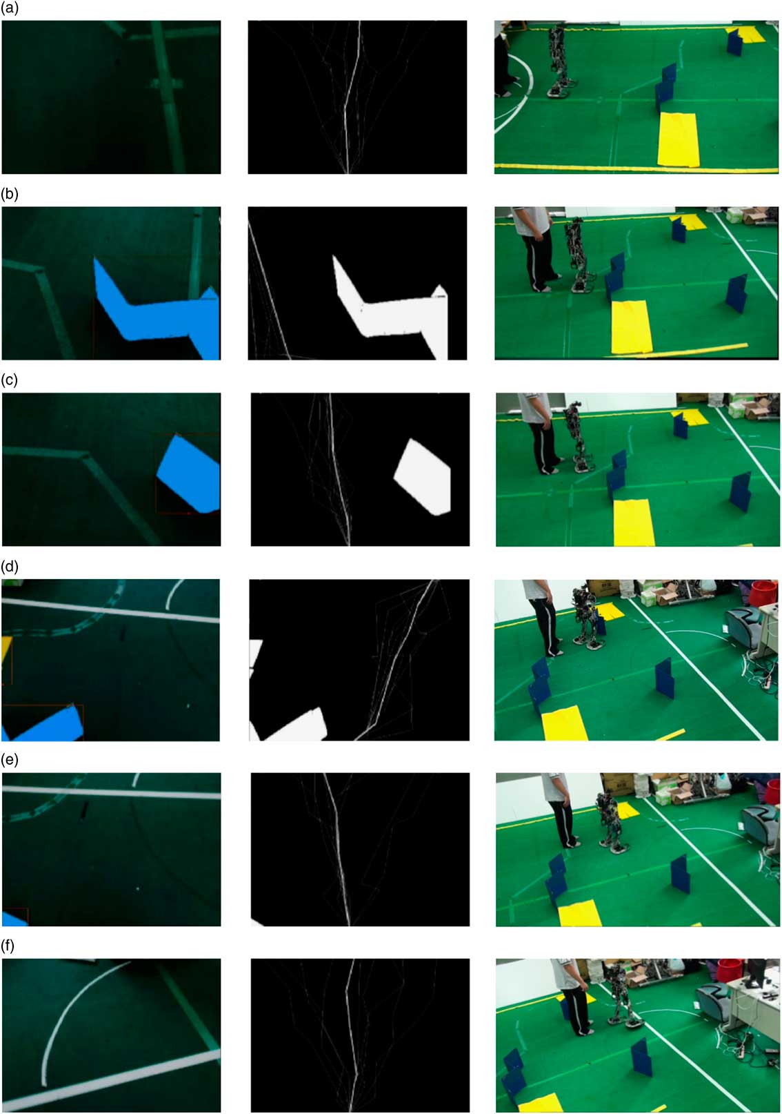
Figure 19 Experimental results. The obstacle run progress is listed sequentially in (a)~(f)
4.3 Competition results
Figure 20 shows the competition results from FIRA HuroCup 2015. According to the rules, all the obstacles are randomly placed on the field. By using the proposed method, the robot accomplished the obstacle run event in real time. Moreover, the robot also won the championship at the FIRA HuroCup Obstacle Run Event 2015 in South Korea.

Figure 20 Competition results at FIRA HuroCup 2015. The competition progress is listed sequentially in (a)~(i)
5 Conclusions
In this paper, the migrant-inspired path planning algorithm (H-PSO) is designed and implemented for the humanoid robot to accomplish the FIRA HuroCup Obstacle Run Event. The PFN method, the PSO, and the FLC are designed and combined in the proposed algorithm. By adopting the generated forces of the PFN method, the convergence speed is increased for this issue. The feasibility and the performance of the proposed method are also validated by the simulation, experimental, and competition results. Compared with other methods, the proposed algorithm provides fastest convergence speed and obtains the highest fitness values in the simulation results. Eventually, the proposed method produced good results in the 2015 FIRA HuroCup Obstacle Run Event.
Acknowledgments
This work was supported in part by the Ministry of Science and Technology, Taiwan, ROC, under grants MOST 103-2221-E-006-252 and MOST 104-2221-E-006-228-MY2, and in part by the Ministry of Education, Taiwan, within the Aim for the Top University Project through National Cheng Kung University, Tainan, Taiwan.


