2.1 Bayesian networks

BNs are an efficient tool for reasoning probabilistically (Pearl, Reference Pearl1988). A BN B = (N, V, E, P_N) provides a factorized joint probability distribution on a set N of RVs. The network has a directed acyclic graph (V, E), where each vertex v_i ∈ V (also called a node) represents a specific RV n_i ∈ N. A directed edge e_j ∈ E represents a conditional dependency between two RVs. Each RV n_i has two or more mutually exclusive and comprehensively exhaustive states. For each RV n_i, there is a set of zero or more RVs called the parent set of n_i, Pa(n_i), each having a directed edge to n_i. An RV with parents is also called a child RV. A PC is the assignment of a specific state to each RV in the parent set. Finally, there is a collection P_N of probability functions that assigns each RV a conditional probability P(n_i |Pa(n_i)) to each state of n_i for every PC in the parent set. The joint probability distribution for a set of specific RV states in (N, P_N) is

(1)\begin{align}\mathop \prod\nolimits_{{n_i} \in N} P(\left( {{n_i}} \right)|Pa\left( {{n_i}} \right)) \end{align}

2.2 Key knowledge representation concepts

The RVs in a BN model knowledge representation concepts. Following Brachman and Levesque, we use five basic concepts to define the elements of a knowledge base that describes some domain. The first is entity or named individual. These are the domain elements. Each entity is typed, using a unary predicate that assigns each entity to a class. The features of an entity are described by attributes (also called datatype properties), each one assigned by a unary predicate. Relationships between entities are described by n-ary predicates. Finally, functions are a special form of relationship, in which a specific entity is assigned from a mutually exclusive collectively exhaustive class of entities (Brachman & Levesque, Reference Brachman and Levesque2004). For a specific domain, one can develop an ontology to define the domain’s entities, attributes, and relationships (Gruber, Reference Gruber2009). The Web Ontology Language (OWL) is a standard and widely used ontology language (McGuinness & van Harmelen, Reference McGuinness and Van Harmelen2004; Consortium, 2012). A specific BN has propositional expressivity—both the number of RVs and parent set of each RV are fixed. If the number of entities can vary, the model must be restructured to account for the change. This limits a BN’s applicability because it cannot model most dependencies between a variable number of domain entities (Milch & Russell, Reference Milch and Russell2010). BN modeling capabilities that can automatically restructure a BN as the number of involved entities change are said to have first-order expressivity.

2.3 First-order expressive probabilistic logics

Development of first-order BN capabilities has been part of a larger effort to develop probabilistic logics with first-order expressivity. These logics combine first-order logic (or a fragment of first-order logic) with uncertainty reasoning (Poole, Reference Poole2011; Russell, Reference Russell2015). Modeling capabilities for first-order probabilistic logics developed along three tracks: probabilistic description logics (DLs), probabilistic logic programming, and probabilistic graphical models.

DLs are fragments of first-order logic with an emphasis on computational tractability and decidability. DLs are strongly associated with knowledge representation and reasoning efforts (Baader et al., Reference Baader, McGuinness, Nardi and Patel-Schneider2003). They provide a semantic and reasoning basis for variants of the OWL. Early work in extending DLs probabilistically started with P-Classic (Koller et al., Reference Koller, Levy and Pfeffer1997). Probabilistic versions of the most expressive DL languages used in OWL are P-SHOQ and P-SHOIN (Lukasiewicz, Reference Lukasiewicz2008). The logic programming track extended the concepts of expressive logical programming languages like Prolog by adding the ability to address probabilistic uncertainty. Examples include Independent Choice Logic (Poole, Reference Poole1997), Bayesian Logic (Milch et al., Reference Milch, Marthi, Russell, Sontag, Ong and Kolobov2007), and Church (Goodman et al., Reference Poole2008). The third track, probabilistic graphical models, extended graphical models from a fixed-entity or limited variable entity count propositional logic level to a first-order level. It is divided into two subtracks: Markov networks and BNs. Markov networks, in contrast to BNs, use undirected graphs, allowing them to model cycles. This is useful in domains such as visual recognition, social network analysis, and object identification. The downside is that the potential functions must be specified globally, so changing any part of the network requires a respecification of all the potentials assigned to every node (Koller & Friedman, Reference Koller and Friedman2009). Markov networks have propositional expressivity and their extension to first-order logic is known as Markov logic networks (Richardson & Domingos, Reference Richardson and Domingos2006; Domingos & Lowd, Reference Domingos and Lowd2009). First-order BNs are an active research area that has resulted in diverse modeling frameworks, such as object-oriented Bayesian networks (Koller & Pfeffer, Reference Koller and Pfeffer1997), probabilistic relational models (PRMs) (Getoor et al., Reference Getoor, Friedman, Koller, Pfeffer and Taskar2007), probabilistic entity-relationship models (Heckerman et al., Reference Heckerman, Meek and Koller2007), object-oriented probabilistic relational modelling language (OPRML) (Howard, Reference Howard2010), and MEBN (Laskey, Reference Laskey2008).

First-order modeling frameworks based on BNs have three primary characteristics beyond a BN. First, they have a template structure that identifies the RVs and the dependencies between RVs in a model. There is a basic requirement that the set of templates be logically consistent. Second, there is a database that identifies the entities in a specific instance of the model and has findings (evidence) on zero or more RVs of specific entities. Third, they have a specification for how the LPD is created for each RV, given a varying number of parent entities for each RV. In addition, a first-order BN representation requires a corresponding inferencing approach. One approach is to create a grounded Bayesian network for a given template structure, database, and LPD specification. The grounded BN is an ordinary BN. It can be queried and updated using standard BN inference algorithms (Mahoney & Laskey, Reference Mahoney and Laskey1998) (Pfeffer, Reference Pfeffer1999). Grounded BNs can be very large and may be computationally intractable. Another approach is lifted inference, which limits the degree of grounded modeling required (Kersting, Reference Kersting2012; Kimmig et al., Reference Kimmig, Mihalkova and Getoor2015). This paper adopts the grounding approach, as it aids in visualizing the patterns.

A recent review of first-order BN modeling frameworks found three viable implementations: PRMs, MEBNs, and OPRML (Howard & Stumptner, Reference Howard and Stumptner2014). A review of probabilistic reasoning methods for use in automated driving situational awareness identified MEBN, with a fuzzy logic extension, as the most broadly capable approach for probabilistic first-order logic modeling (Golestan et al., Reference Golestan, Soua, Karray and Kamel2016).

There are three common assumptions made regarding multiple entity instances of an RV in any first-order probabilistic logic: nonuniqueness, exchangeability, and nonattribution. Nonuniqueness is a strong requirement that any set of instances of an RV modeled with a template has the same set of states and LPDs. This assumption is core to any template-based approach. Exchangeability means that the order of a set of parent RVs has no effect on the child RV’s probability distribution. If ordering is important, the template design, database, and/or the LPD specification require additional features to address this. Nonattribution means that the child RV’s LPD only depends on the numbers of parent RVs in each of their possible states and does not depend on which specific parent instances are in which state. In our patterns, several will violate nonattribution, which places an extra requirement on the LPD specification.

3.1 Multi-entity Bayesian networks

Although the patterns presented in this paper are generic to first-order probabilistic representations, we adopt MEBN constructs as visualization tools. MEBN represents the world as a collection of inter-related entities, with relationships between them. Entity and relationship knowledge are modeled as a collection of reusable knowledge elements, called MEBN Fragments (MFrags). A MEBN Theory (MTheory) is a set of well-defined MFrags that collectively satisfy first-order logical constraints ensuring a unique joint probability distribution (Costa & Laskey, Reference Costa and Laskey2005). Formally, an MFrag F = (C, I, R, G, D) consists of a finite set C of context value assignment terms; a finite set I of input RV terms; a finite set R of resident RV terms; a fragment graph G; and a set D of LPDs, one for each member of R. The sets C, I, and R are pairwise disjoint. The fragment graph G is an acyclic directed graph whose nodes are in one-to-one correspondence with the RVs in I∪R, such that RVs in I correspond to root nodes in G. LPDs in D specify the conditional probability distributions for the resident RVs (Laskey, Reference Laskey2008).

Figure 1 shows an example MFrag. This simplified example models the informal statement that a student’s performance in a course partially depends on a professor’s teaching ability. In a MEBN, ordinary variables (OVs) are placeholders for entities from some domain. The pentagonal nodes are context nodes. They represent the conditions that must be met for the MFrag to be applicable. In this example, the two IsA context nodes identify the domain class from which an OV takes entities. The context node is an RV specified in another MFrag and stipulates the conditions under which the MFrag is used. Teaches(p, s) is a context node requiring that a specific professor entity must teach a specific student entity for this MFrag to have meaning. The rounded node is a resident node. Each RV is a resident node in one MFrag, which defines its states and provides a LPD defining the probability of each state depending on the state(s) of its parent(s). The trapezoidal node is an input node, signifying that an RV defined in another MFrag is aparent RV of a resident node. An MFrag must have at least one resident node. It can have as many resident, input, and context nodes as a designer wants to incorporate. However, small MFrag sizes facilitate knowledge reuse. An introduction to MEBN can be found in P. C. G. Costa and Laskey (Reference Costa and Laskey2005).

A complete MEBN theory also includes a database of known entities and facts. In the example above, this could be that ‘Kathy is a professor’, ‘Paul is a student’, ‘Kathy teaches Paul’, and ‘Kathy has good teaching abilities’. The implemented MEBN tool (UnBBayes MEBN, Matsumoto, Carvalho, Ladeira, et al., Reference Matsumoto, Carvalho, Ladeira, da Costa, Santos, Silva, Onishi, Machado and Cai2011) uses a MEBN-based probabilistic extension of OWL to support part of the overall knowledge base design (Costa, Reference Costa2005; Matsumoto, Carvalho, Costa, et al., Reference Matsumoto, Carvalho, Costa, Laskey, Santos, Ladeira and Fung2011; Carvalho, Laskey, and Costa, Reference Carvalho, Laskey and Coasta2017).

The MFrags are templates for the grounded BNs. In MEBN, grounded BNs are known as situation-specific BNs. The grounding approach is query specific, in which only the network required to address a specific query about a specific set of entities is instantiated. RVs that add no information are not instantiated (or are pruned prior to network compilation). This results in the minimum network size to address the query. But it requires constructing a new grounded network if the query changes. Section 4.2 provides the specifics of model grounding required to understand our patterns. An alternate approach used in PRMs is a global approach, in which every RV applicable to every entity in the database is instantiated, creating large grounded networks. It has the advantage that any query about any entity in the database can be addressed without recreating the network. A full description of construction algorithms in use can be found in Mahoney and Laskey (Reference Mahoney and Laskey1998) for query-specific construction and Pfeffer (Reference Pfeffer1999) for global construction algorithms.

3.2 Local probability distributions

A key feature of our patterns is that they constrain the choices for the LPD associated with that pattern. Every RV in a BN has an LPD that defines a probability for each RV state, conditional on the states of the parents. In a propositional BN, where each RV has a fixed number of parents, the LPD is most often expressed as a conditional probability table (CPT). As a first-order expressive probabilistic model can vary in the number of parents, the LPD is instead a function that specifies, for each instantiated RV, how to assign a conditional probability based on the number of parents and their specific states. Where the number of possible entities is small, or where the effective influence of the number of parents can be capped (such as ‘for 5 or more parents with state = X’), the LPD can be explicitly defined as a CPT. Otherwise, the LPD must have a functional form that defines the conditional probabilities. The LPD can be specified using a scripting language.

A significant problem in first-order expressive probabilistic models is the exponential growth in the number of probabilities required as the number of parents increases. This creates problems for probability development, whether via expert elicitation or machine learning. If the LPD involves a complex degree of interactions among the parents, the problem is unavoidable. But for many problems, the LPD can be simplified by exploiting one or more independence conditions. These are context-specific independence (CSI), independence of causal influence (ICI), and aggregators. Taking full advantage of these independence conditions requires specific capabilities for developing a specific LPD.

CSI occurs in an LPD when only a portion of the PC is needed to establish the child RV’s probabilities. For example, the following conditional probability exhibits CSI. Although each has five parents, the state of parent A limits the influence of the other parents to only one other parent, such as

(2)\begin{align} {\text{P}}\left( {{\text{child RV | A = state1, BCDE}}} \right)\!{\text{ = P}}\left( {{\text{child RV | A = state 1, B}}} \right){\text{ (depends only on state of B)}}\end{align}

ICI requires that two or more parent RVs do not have synergistic interactions with each other in the child RV’s LPD. That is, the influence of each parent on the child RV’s state probabilities does not depend on the state of any other parent. ICI models can be expressed using combining rules. Figure 2(a) shows the structure of an ICI model using a combining rule approach. The parents are the X_is. Each X_i stochastically influences the state of a Y_i. As there are no arcs from any X_i to Y_j, i ≠ j, each Y_i is conditionally independent of all parents except X_iFootnote ¹. The states of the Y_is are then combined using some type of deterministic functional equation. The first combining rule model (noisy-or) used the logical OR as the deterministic equation (Pearl, Reference Pearl1988). Other commonly used combining rules are the noisy-and, noisy-max, and noisy-min. ICI models can be built using any Boolean function—see Lucas (Reference Lucas2005) or van Gerven et al. (Reference Gerven, van Lucas and van der Weide2008). Some Boolean ICI models can be extended to multiple state models by exchanging the Boolean deterministic function for its algebraic extension (e.g. using Max instead of Or). ICI models are widely used, especially in the medical domain. See Bermejo et al. (Reference Bermejo, Díez, Govaerts and Vaerenberg2013), Magrini et al. (Reference Magrini, Luciani and Stefanini2016), or Anand and Downs (Reference Anand and Downs2008) for examples and recent extensions. There also has been some work on allowing a limited degree of LPD-level interaction between parents. This is especially the case in the medical domain, where drugs may have positive or negative synergy when used together (Woudenberg et al., Reference Woudenberg, van der Gaag and Rademaker2015).

Figure 2 Independence of causal influence-based combining rule model and aggregator model

In an aggregator, the states of the PCs are first combined via one or more deterministic functions, and the results are used to create a deterministic RV. This RV then interacts stochastically with the child RV (see Figure 2(b)). A very simple example is to estimate a student’s likelihood of success in a graduate program based on her performance in her undergraduate courses. An aggregator would average the grades in all courses (the X_is) to obtain a single value (the grade point average, in the Y RV). Then, there would be a probabilistic correlation between GPA and success in a graduate program. Both ICI models and aggregator models depend heavily on the use of deterministic functions. Where the deterministic function produces a fixed or limited number of states, the stochastic function can be a CPT. If the aggregator produces a variable number of states, a functional probability model is often used. Here, the aggregation output (variable Y) provides the parameters of the function. This model is either a standard probability distribution (e.g. binomial, logistic, Poisson, etc.) or a custom-built probability model, usually based on some form of machine learning or expert elicitation. There are several examples in Kazemi et al. (Reference Kazemi, Fatemi, Kim, Peng, Tora, Zeng, Dirks and Poole2017). Kazemi et al. (Reference Kazemi, Buchman, Kersting, Natarajan and Poole2014) discuss the sensitivity of various probability models to different aggregator functions as the size of the underlying aggregated population changes. The patterns described below often use aggregation at the PC level. A good introduction to both ICI and aggregator models (called simple canonical models) is by Dıez and Druzdzel (Reference Dıez and Druzdzel2006).

Under conditions of nonuniqueness, where all P(Y_i|X_i) are identical, it is possible to implement a combining rule as an aggregator. It can be done even when the X_is are uncertain. Because of this feature, it has become common to group both aggregators and combining rules as aggregators, especially in the PRM community (e.g. Raedt et al., Reference Raedt, Kersting, Natarajan and Poole2016). However, combining rules can also be applied to models where nonuniqueness holds, that is, the P(Y_i|X_i) are not identical, while aggregators cannot.

3.3 Constraints

Often the problem environment has constraints among the attribute and/or relationship instances that must be captured to accurately model the problem. They fall into two categories: restrictions on the state of one or more parents, based on the state of other parent nodes, and restrictions on the state of a child RV based on the state of one or more other child RVs. Constraints between parents and a child RV are enforced in the child RV’s LPD. The relationship modeled between two OVs in an RV is not inherently constrained by the form of the RV. But in the intended understanding of the relationship, there may be a constraint on the states among the entities instantiating a particular RV. There are three ways to enforce constraints in a BN: direct parent dependency, constraint node, or embedded constraint, as shown in Figure 3.

Figure 3 Constraint modeling options

The first approach is to add dependencies among the parent RVs that implement the constraint. Figure 3(a) shows a grounded model with parent dependencies. To do this requires a total order on the entities in the classes affected by the constraints. The order may be natural (e.g. greater than, less than, etc.) or arbitrary. While a natural ordering is limited to one class, an arbitrary ordering can extend across multiple classes. In this approach, dependencies among the parents are used to enforce constraints. For a one-of constraint, the core LPD is that any instance of the Constrained_Entity RV type will have state False if any of its parents have state True. Assuming a uniform prior probability across all the instances of that RV type is appropriate, the probability that each entity in the order has the constrained condition is

(3)\begin{align}{\text{P}}\left( {{\text{Constrained_Entity - X}}\,{\text{ = }}\,{\text{True}}} \right){\text{ = 1 /}}\left( {{\text{cardinality}}\left( {{\text{entity set}}} \right){\text{ -- Order number + 1}}} \right)\end{align}

While this example is simple, more complex constraints can require a more complex LPD, which is harder to understand. Constraint nodes provide an easier approach. These are nodes added to the BN specifically to implement the constraint(s). Constraint nodes can be used to enforce constraints among any set of nodes. Figure 3(b) above shows the basic pattern for a global constraint node. There is a Boolean node, called the constraint node, with arcs from the nodes on which the constraint(s) are enforced. In the constraint node LPD, the conditions for which a PC meets the constraint(s) maps to Allowed (e.g. in the example, exactly one Constrained_Entity RV has state = True). Otherwise, it maps to False. The constraint node has a database finding that the state of the constraint node must be Allowed. This enforces the constraint. The constraint nodes and direct parent options are functionally equivalent, and if the constraint node is absorbed into its parents, then one converts Figure 3(b) into Figure 3(a). It is generally easier to specify the LPD in terms of allowable and unallowable PCs, making the constraint node easier to implement. This is especially the case when a constraint applies across multiple classes or multiple types of RVs. A constraint node may be total or partial. The first is illustrated in the figure above, in which a single node applies the constraint to all nodes of one or more RV types as a groupFootnote ². A partial constraint node applies to a subset of the nodes, and there may be multiple such nodes to enforce the overall constraint. Constraints can also be applied to a set of child RVs, using either approach. For instance, if each entity that instantiates a child RV must have a unique state, then a global or set of partial constraint nodes can be used to implement the constraint.

When a constraint node is used, it adds additional nodes to the BN and increases the complexity of the network. For constraints among parent nodes (including subsets of parent nodes), it is possible to embed the constraints into the LPD of the child RV. This is done in the patterns described in Section 4 below when a constraint is necessary. The set of states of the child RV is augmented with a new state whose purpose is to implement one or more constraints among the parent RVs. The patterns below use NA (for ‘Not Allowed’) when a constraint exists. For each child RV instance that has an NA, there is a finding that the NA state must be False, for example, it is not allowed. Figure 3(c) above shows the use of an embedded constraint. The LPD is constructed in two parts. First, all the PCs that have constraint violations are mapped to NA (same approach as for a constraint node). Then the remaining PCs are mapped to the child RV states with the conditional probability appropriate to that PC.

The above approaches have a problem if one is implementing a 1-of-n constraint, as in the example. If prior information assigns different probabilities to the nodes being constrained, then the constraint approaches described above will change the value of those nodes. Fenton et al. (Reference Fenton, Neil, Lagnado, Marsh, Yet and Constantinou2016) discovered a relatively straightforward way to correctly initiate the prior probabilities.

4.1 Pattern content definitions

Following the knowledge representation concepts described in section 2.2, our patterns use RVs that model an entity’s attributes, relationships, and functional relationships. This leads to three RV types:

• Attribute RV (A-type), with a single OV, model attributes. For each entity in a class, this unary RV assigns a probability to each possible state of an attribute for that entity.

• Relationship RV (R-type) with two OVs. This binary RV models relationships such as isFriendsWith(x,y), read ‘x is Friends with y’. These use Boolean states.

• Functional RV (F-type), model functions, has two entity variables. One is the OV, the entity that is the subject of the RV. Since an F-type RV has entities as states, there is a second variable, called an SV, that represents the entity states of the RV.

The RV MachineLocation(m) is an F-type RV. It models a functional relationship between a specific machine entity and the room it is located in. When one needs to know what the SV is, the RV is annotated as MachineLocation(m)/r, where r is the SV. It is possible for the same variable to be an OV for one RV and the SV for another RV. If two RVs in a template have the same OV, this signals that they are intended to model the same entity. If they have different OVs from the same class, the entities may be the same or different. Context variables may be necessary to enforce the desired distinction (e.g. (x ≠ y)).

First-order expressive BNs can use RVs with more OVs than shown above. But this work began with the RV arities described above for two reasons. First, as will be seen below, they provide sufficient modeling complexity to explore a wide range of applications. Second, BN development benefits from reusing a domain-specific ontology. Many ontologies are developed using OWL (Sections 2.2/3.1), which is also limited to these arities. Modeling more complex relationships is future work.

4.2 Dependency models

To uncover patterns useful for first-order expressive BN modeling, we developed dependency modeling. This approach explored the dependencies between the attributes and relationships in a set of entities. Exploring dependencies at this general level means that the patterns are applicable to a wide range of problem domains. Dependency modeling examines the range of interactions between different combinations of the RV types described above to determine both the kinds of structural arrangements they can create in the grounded models and in the LPD creation behaviors they enable. For example, an attribute can have an influence on the state of a relationship, or two relationships can interact to influence the state of a third relationship. The dependency models are developed at the template level, and then a possible grounded model is generated from each template. The resulting grounded models were mined to identify common patterns among them. In our effort, we specifically modeled all templates where an RV has a single parent, and where it has two parents. We are modeling different parent-child interactions but are not modeling any extended sequences, such as RV1 → RV2 → RV3 or RV1 ← RV2 → RV3.

Since we use three RV types, there are 9 possible combinations with one parent, and 18 possible combinations with two RV parents, as shown in Figure 4. Each combination is a dependency model. The child RV (also called the target RV—this is the one for which the LPD is defined) is always RV3, and A/F/R identify the RV type, per Section 4.1 above. In the two-parent-type models, the numeric identifiers for the parents (e.g. F1, R2) are reversible (e.g. F2, R1). Also, if both parents have the same RV-type (e.g. an F-type RV), the two RVs may be the same or they may be differentFootnote ³. The dependency models in Figure 4 do not include OVs or SVs. Different variable combinations may be used in the same model. For the one-parent-type models, there can be from one to four distinct OV/SVs, depending on RV types used. The two-parent-type models can have up to six distinct OV/SVs (from every RV has the same OV/SV to each RV has a different set of OV/SVs).

Figure 4 Possible dependency models with one or two parent RV types representing entity attributes (A), functional relationships (F), or binary relationships (R) in the template

Different variable combinations can result in different grounded models, so it is important to understand how the construction algorithm uses the template and database to create the grounded model. We assume the use of a query-specific construction algorithm, rather than creating a grounded model able to address any query. The query is of the form ‘What is the state of RV3 for specific entity “a” or “a and b” (if RV binary)?’ The query-specific construction algorithm begins with the query RV. One instance of RV3 is instantiated with the queried entity(ies). Then, the algorithm looks at the OVs in each parent node in the templateFootnote ⁴. If the OV of an RV is the same as for the child RV, it is bound. The algorithm creates one instance of that RV, with the same entity as the child RV. If the OV is different than the child RV’s OV, it is free. One parent instance of that RV is instantiated for every entity in the OV’s classFootnote ⁵. When the parent is a binary R-type RV and the child is unary, then if they have a common OV, the R-type parent will instantiate as many RV instances as there are entities in the free OV’s class. The common OV is bound and will have the same entity as the child RV. If an R-type RV has two OVs different from the child RV’s OV, the algorithm will instantiate m * n instances, where m and n are the cardinalities of the two classes represented by the OVs. For a template, the algorithm completes when it has instantiated every RV in the template with the number of bound and free OVs.

Different combinations instantiate different parent sets for the same basic dependency model. Figure 5 gives an example, where there is the same dependency model (A1, F2, A3) but the order of the variables for the F2 RV type is inverted. In this modeling, A(x) means x is the OV of the RV, while F(x)/y means x is the OV and y is the SV. Figure 5 models the effect of a room’s temperature on a machine’s operational status. A room’s temperature affects a machine’s status only when the machine is in that room. Here, one is uncertain as to which room a specific machine is in. The database has four rooms and four machines. The query here will be on the status of machine M1.

Figure 5 Inverting the variables in RV F2 results in a different pattern

RoomTemperature and MachineStatus are both attribute-type RVs and are identical between the two examples. The F2 RV has its OV and SV classes inverted between the two examples. The actual F-type RVs (MachineLocation and RoomOccupant) are inverses of each other. This results in two different parent sets. In Figure 5(a), the F-type RV has the same OV as the child. One instance of that RV is instantiated. In Figure 5(b), it has a different OV, so four instances are instantiated. These are two different structuresFootnote ⁶.

Different variable combinations also affect the understanding of what is being modeled. There are collectively 39 distinct variable combinations (or cases) for the one-parent-type dependency models and 414 cases for the two-parent-type dependency models. However, finding meaningful interpretations for many of these variable combinations is difficult, especially when each RV has OV/SVs that are different from every other. Consider the following instantiation for the template in Figure 1: if ‘Kathy has good teaching abilities’ and if ‘Kathy teaches Mark’, then ‘Mark has good student performance’. Consider now that the template has four OVs (say p1, p2, s1, s2), instead of two. An instantiation then could be If ‘Kathy has good teaching abilities’ and if ‘Paulo teaches Mark’, then ‘Rommel has good student performance’. Both examples have the same dependency model, but only the first one seems to make sense. In the second case, one does not see the connection between the entities being modeled. It is possible to identify circumstances where there exists enough shared background knowledge that such an entity combination would make sense. But most often, one expects there is an interaction between the specific entities identified in the model. This led to a search for variable combinations that carried meaningful semantic information.

In looking at the possible variable combinations, we first eliminated the cases where there was only one variable used by all RVs. These cases create very simple models (only one instance of each parent-type is instantiated) and require all relationships and functional relationships to be reflexive. For the remaining cases, it became apparent that the concepts modeled by RV combinations can make sense when they have common entities between them. There are a few cases where one can use domain background knowledge to make sense of cases where each RV had different variables, but they were eliminated from the analysis because of this domain specificity. One sharing item was that the child RV must share its variables with the one or more of the parents. The only exception was for the one-parent dependency models where the parent is an attribute and the child is either a relationship or a functional relationship.

This sharing enables a meaningful connection between the concepts modeled in the parent and child RVs. For one-parent-type dependency models, the effect of this requirement is that all one-parent-type dependency models have two distinct variables.

For two-parent-type models, we found three schemes for such entity sharing. The first is an enabling scheme, which occurs when two RVs model attributes of different entities, and the third RV models a relationship or functional relationship. This RV can be either a parent or a child, and it shares variables with the two attribute RVs. This licenses the dependency between the two attribute RVs. Both examples in Figure 5 are examples of this scheme. The second variable scheme is a pass-through scheme that applies to combinations of relationships or functional relationships. It occurs when there is a dependency between three relationships where the one parent has entity x in a relationship/functional relationship with entity z and the other parent has entity z in a relationship/functional relationship with entity y (either the same kind of relationship or different). There then can be a meaningful relationship between x and y, captured in the child RV. If the three relationships are identical, and the entities are from the same class, then this is a transitive relationship. However, there is no requirement that they are identical. An example is if hasChild(x,z), and if isParentOf(z,y) then isGrandparentOf(x,y).Footnote ⁷ Pass-throughs also support dependencies between parent relationship RVs and a child attribute RV. The third variable scheme is a common variable. Here, the parent RVs share a variable in the same variable position, and the other variable in each parent is shared with the child RV. This enables a dependency for a relationship for the other two variables. The effect of these schemes is to limit two-parent-type models to having two or three variables.

Applying these variable sharing requirements to the dependency models shown in Figure 4 reduced the number of meaningful variable combinations from 453 to 41 cases. Then, there was an attempt to build a scenario for each case. In four cases, generalizable scenarios could not be found. Almost always, those cases required additional relationships to license the dependencies between the OVs. For instance, no meaningful scenario could be found for cases where one or two attribute-type parents influenced a child attribute RV without assuming a relationship between the OVs. This required that a third parent- type RV be added. In addition, no scenarios could be found for two F-type RVs influencing an A-type RV, or an F-type RV and A-type RV influencing a child F-type RV. This reduced the number of modeled cases to 37.

For each modeled case, the structure of the grounded model for the scenario and the behavior used in LPD creation were identified. Recurring behavior patterns were noted across the 37 cases. They grouped themselves into three major categories: selector, existential selector, and embedded dependencies. The following sections describe each pattern and include a figure showing one or two examples. Because the patterns recurred across the 37 cases, not all are shown in the examples. In general, the figure includes

• Dependency model case with a generic variable combination (x, y, z)

• Template with the scenario model. Scenario is described in the text

• Query being addressed in the scenario

• Knowledge base with the entities, and a grounded model based on those entities

• Constraints enforced in the grounded model. All constraints are enforced using an embedded constraint node approach

• Basic dependency between parent(s) and child RVs

• Required LPD behavior.

4.3 Selector patterns

Selector patterns are two-parent-type models where the template has either an F-type or A-type RV with the same OV as the child RV. Because it has the same OV as the child, only one instance will be instantiated. This instantiated RV acts as the selector. It identifies a condition that the instantiated RVs of the other variable type must meet for the instantiated variables to have an influence on the child RV. There are three selector patterns: Select-One, Select-Match, and Child-Select.

Figure 6 Select-One pattern examples, showing context-specific independence. Selector in Example 2 chooses a row of possible mothers

In the Select-One pattern, the selector is an F-type RV and the SV of the selector is an OV for the other parent RV-type. In this pattern, the LPD always exhibits CSI. Figure 6 shows two examples of this pattern. Example #1 is a well-known pattern used to resolve reference uncertainty (Getoor & Grant Reference Getoor and Grant2006; Getoor et al., Reference Getoor, Friedman, Koller, Pfeffer and Taskar2007). The example begins with the basic pattern, in which an attribute RV A1 with entities from the class represented by OV y has an influence on a specific entity with attribute RV A3 (whose OV may be from the same or different class than the OV in A1). The functional relationship in RV F2 enables the dependency between A1 and A3. The template in example #1 captures the fact that a machine is in a particular room (as defined in MachineLocation(M)), and the room has a temperature of either normal or hot. The room’s temperature affects the probability of the machine’s status, either normal or overheated, per the associated table. Here, one is uncertain about which room the machine is in but does know that it must be in one of four rooms. The construction algorithm takes the template and the database entry that there are four possible rooms to create the grounded model. In the LPD, MachineLocation_M1 acts as a selector. For each PC, it identifies the one room whose state will establish the probabilities for that PC, using the probabilities expressed in the table. The figure includes a representative set of LPD behaviors visualizing the CSI characteristics. A key LPD behavior is to perform indirect referencing. Here, the state of the F-type selector is the room of interest. Indirect referencing allows us to say State(RoomTemp(State(MachineLocation))) to indicate we want to know the room temperature of the room that is the state of the MachineLocation RV.

While example #1 is an attribute-to-attribute example, where the selector licenses the dependency, one can create similar patterns with dependencies that include relationships. This is useful when doing probabilistic social network analysis. In example #2, there is a dependency model where an R-type RV influences an F-type child RV, with an F-type RV enabling the dependency. The specific example models the probability that a particular woman is the mother of a child, depending on whether she is married to the father of the child. The template shows three entity classes. The database identifies three men as possible fathers and three women who could each be married to one of the men. The lists of possible mothers and fathers are assumed to be collectively exhaustive. A key constraint is that each man and each woman can be married to at most one person. In the grounded model, the MotherOf RV (the query node) includes an NA state. This model uses an embedded constraint node approach. FatherOf has the same OV as MotherOf, so only one instance is created. FatherOf is the selector. The variables in MarriedTo are free, so it will instantiate |M| * |W|Footnote ⁸ instance RVs.

This example has two interesting features. First, the marriage constraint applies individually to six different people, resulting in six constraints, one for each person in the knowledge base. The constraints are partial constraints across the parent set. Figure 7 visualizes the constraints needed. Each row in the parent set corresponds a specific man, and each column to a woman. In the LPD, constraints are checked first, and the constraint is applied for each man and woman (row and column, respectively). If there is more than one marriage in any row or column, then PC has 100% probability of NA. Constraints can eliminate a significant number of PCs from consideration. Here, there are 1536 PCs; constraint violations eliminate 1434.

Figure 7 Multiple partial constraints by person (man/woman). Segment of model in Example 2

The second interesting feature is that the LPD requires parent entity attribution, knowledge of the specific parent entities that match a specified condition to properly assign the child RV’s state probabilities. For all PCs that meet the constraints, the state of the selector RV, FatherOf, is determined, and the True states of the three MarriedTo RVs with that man are counted. In this case, the count will be either zero or one, as the constraint has already eliminated the PCs that have more than one MarriedTo being True. If the count is zero, then each of the possible mothers will have a uniform probability, 1/|Woman|. If the count is 1, then a 75% probability is assigned to the woman who is married to the father, while the remaining women each receive a uniform share of the remaining probability, for example, 0.25/(|Woman| −1). In this case, the LPD needs to know which specific woman is the married one, because the child RV states also come from the Woman class. Entity attribution is required whenever the child RV is an F-type RV, as its states are entities.

In the Select Match pattern, the selector identifies a state of interest and the LPD examines the other parent type to identify which ones match the selector state. In this case, the selector may be either an F-type or an A-type RV. This pattern requires entity attribution. The selector RV has the same OV as the child RV, so only one instance of the selector variable is instantiated. Figure 8 highlights two examples of this pattern. In the first example, two F-type RVs collectively influence an F-type child RV, and both parent types have the same SV (o). In the example, which room a particular machine is in (the MachineLocation RV) depends on matching information from both the room choices and the selected machine. There are three classes involved: Machine, Room, and Organization, with one machine entity, four room entities, and two organization entities. For this model, there is a requirement that a machine can only be in a room whose tenant is the same organization that owns the machine. This becomes the selector condition that the entities of the other RV type must match. Owner_m1 is the selector, and the states of the child RV are from the same class (room) as the OV for the RV Tenant. We are looking for the behavior COUNT ((State(RV2) = State(RV1)). In the LPD excerpt, one sees this behavior. It has three PCs, each with the state of Owner_m1 being o1. In the first line, the tenant of rooms r1, r2, and r4 is also organization o1. The child RV probability is then 1/Count for each of the rooms that met this condition (r1,r2,r4). The second LPD line shows Owner_m1 state being o2, with only tenant r2 and r3 having the same state. The grounded model shows that MachineLocation_m1 has an NA with probability 0, indicating the existence of an embedded constraint in the LPD that the machine must be in one of the four rooms. However, there are two PCs where this is not possible. In the first, machine m1 is owned by organization o1 while the four rooms are tenanted by o2, while the second PC is reversed. In both cases, the probability of the machine being in any room is zero. The embedded constraint indicates that these two PCs have no meaning in this model. Line 3 of the LPD excerpt shows one of the two disallowed PCs.

Figure 8 Select Match Pattern examples, where the LPD must keep track of the specific entities that meet the selection criterion

In the select match pattern, it is possible for an attribute to be a selector. This depends on exploiting an embedded dependency between two attributes associated with different entities. Example #2 uses the A1-A2-F3 dependency model, with each attribute having a different OV, and the child RV having one parent OV as its OV and the other parent OV as its SV. Let us assume there are three different machine sizes (say large, medium, and small) and three different room sizes (large room, medium room, and small room). The machines can be in any type of room, but a machine is three as likely to be in a room that matches its size than in the most different room. It is twice as likely to be in a room that is nearest to its size. In the example, there are four possible rooms. In the LPD, the probability of being in a specific room depends on the total number of rooms, and on how many rooms have the same size type as the machine, versus a different size type. The probability distribution is determined via a functional probability specification:

(4)\begin{align}{\text{P}}\left( {{\text{room y}}} \right) = \frac{{Match{\text{\;}}Indicator}}{{3\,{*}\,\# {\text{\;}}RoomSizeMatch + 2\,{*}\,\# RoomsNextSize + 1\,{*}\,LeastSize{\text{\;}}Match}}\end{align}

Match Indicator = 3 if size of Room y matches machine size, 2 if size is next best size, otherwise 1.

Note that this LPD requires that every possible size combination be counted before the probability assignment is made. This is called a state counting capability, for example, how many rooms of each size are there. In addition, it also requires entity attribution. In our examples, each match has an equal weight, but it is possible to use weights if the entities are ordered in a manner that allows weighting.

The third selector-based pattern is the Child Select pattern. It applies to certain dependencies that have an R-type RV as the child. In this pattern, one OV in the R-type child RV is the OV of the selector, while the other OV is used to determine whether the PC supports a state of True. Consider example #1 in Figure 9. Whether a belt is owned by a particular organization depends on which machine it is on and who owns that machine. The premise is that the owner of a machine owns all the parts on it. The grounded model shows three machines and three possible owning organizations. BeltLocation is the selector. The LPD acts very much as in the Select-One pattern, in that the selector identifies one instance of the other parent RV type as having influence.

Figure 9 Child Select Pattern examples—requires that the RV instances whose state matches the selector value must also match the child RV’s entity

However, rather than just using the state of that RV instance in the LPD, the LPD compares the state of the parent RV Owner to the second OV of the child RV. If they match, the child RV state is True. Otherwise, it is False. In the figure, the LPD language uses two forms of indirect referencing. The first, State(Owner(State (BeltLocation))), says that the OV entity of Owner is the state of the BeltLocation, where BeltLocation states are M1, M2, and M3. The second, OV2(BeltOwnedBy), identifies the entity instance in the second OV position (counted from the left) of the RV inside the parentheses. The full LPD can be read as

• If the state of Owner, whose entity is the state of BeltLocation, equals the entity of the second OV position of BeltOwnedBy, then the probability of True is 1.

An indirect referencing capability is needed when dealing with entity states from a possibly varying list.

Example #2 shows a more direct variant. In this case, the selector itself must match the child RV’s OV. The model addresses whether a person (William) has a son (Jamie). The available information is that there are three people who are potential fathers of a child, and the possible sex of the child. There are two conditions that must be met. First, the selector FatherOf must itself match a criterion. For the child RV to be True, the possible father must be the same as the instance of the Father OV in the child RV. Second, the sex of the child must be male. In this case, one OV in the child RV specifies the entity of interest (the Child class OV), while the other OV is a condition that must be met by the selector.

4.4 Existential selector patterns

The second pattern category, Existential Selector, involves either an R-type or F-type RV. If it is an R-type RV, one or both of its OVs will be the same as for the child OV(s). If the child RV has only one OV (A-type or F-Type), one of the R-type’s OV will be free. If there is an F-type RV, it is that RV’s SV, not OV, that will match the child RV’s OV. These patterns differ from the selector patterns in that they instantiate multiple instances of the selector RV, instead of only one. Each existential selector determines whether a specific instance of the second RV type has an effect or not. Uncertainty of a relationship’s existence is a form of property uncertainty, hence the existential name (Poole, Reference Poole2011). These patterns use a variety of counting behaviors. There are three existential selector patterns: Existential-Paired, Multi-Existential, and Child Existential. In the Existential Paired pattern, a distinct instance of an existential selector is paired with an instance of the second RV type in the template. Example #1 of Figure 10 gives a paradigmatic example. The premise is that student’s overall grades depend partially on his professors’ teaching abilities. Assume there are four possible professors, and each professor has either Excellent or Mediocre teaching abilities. Only the ones that teach the student will influence his grades (Teaches is the selector). Hence, there is a pairing between each instance of the relationship RV Teaches(p,s) and the attribute RV TeachingAbility(p) for that professor entity. A possible LPD when the A-type RV has only two states uses a k-out-of-n aggregator model, where n is the total number of the existential selector instances that are true. For those professors that teach the student, k is the number of teachers with excellent teaching ability. Note the NotAStudent state for cases where no professor teaches the purported student. A probability value is attached to each k-out-of-n state, as established by expert judgment, data learning, etc. While this example has binary states for both the attribute and child RVs, it can readily be extended to multiple states. A k-out-of-n count then becomes a state count.

Figure 10 Existential Paired Pattern examples—each attribute or relationship RV instance that could influence a child RV is paired with the relationship instance with the same entity to determine whether that entity has an effect

The second example is a refinement, where the entity associated with ParentOf can be refined to FatherOf, if the entity is male. A key item to making this model work is to ensure two constraints are properly accounted for. First, there must be exactly two biological parents. Second, one parent must be male and one female. One can also see that if the relationship existential selector variable has an enforced many-to-one constraint, then this pattern gives an equivalent result as the reference uncertainty multiplexor in the Select One pattern. For example, the SonOf(f,c) RV, where f is the biological father class and c is the child class, is constrained to having only one father per child instance. This constrained relationship could also be modeled as FatherOf(c).

The model shown in Figure 5(b) is also addressed using an Existential Paired Pattern, using the approach in Example #2 above. In that case, the constraint is that each machine can only be in one room. The embedded constraint in Figure 5(b) enforces that constraint.

In the Multi-Existential pattern, each selector instance is applied against multiple instances of the second RV type. Rather than pairing between specific instances, each selector works across subsets (or all) of the instances. Example #1 in Figure 11 models the case that a woman has one or more children, based on whether the woman is married to a man and then counts how many children that man has. There is also a default probability value in case the woman is not married. There is a constraint that the woman of interest can be married to one man or not be married at all. This is modeled by an embedded constraint in hasChild, as indicated by the NA state. Note that in the grounded model, there is a 25% probability that the woman is not married. isMarriedTo acts as an existential selector, but there is no one-to-one pairing between isMarriedTo and FatherOf. Rather, for each instance where isMarriedTo is True, one counts how many FatherOf RVs have the same entity as its state as the husband in isMarriedTo. A probability value is based on that count. Example #2 shows the pattern when one relationship influences the state of another relationship. Here, one is assessing who the first author is on a paper, based on the paper’s topics and the areas of topical expertise of various possible authors. This example includes simplifying conditions that the list of possible first authors and the list of topics are complete. The existential selector is the hasTopic RV, which identifies the possible topics of a paper of interest. For each topic, there is an associated probability that a particular professor has expertise in that topic. The LPD here counts the number of professors that have expertise in a particular topic area. The higher the count, the less likely any particular professor is the first author. However, if the paper has multiple topics, then added weight is given to those professors who have expertise in more topics.

Figure 11 Multi-existential Pattern examples—each selector acts across some or all of the other RV’s instances

The Existential Child pattern is like the Child Select pattern discussed above, in that there is a dependency between the child RV’s OV instance(s) and the selectors’ states. Instead of a single selector, there are multiple existential selectors. Figure 12 example #1 assesses whether two people are married based on the number of common children they have. In the example, there are three children and three possible mothers and fathers. There is an assumption that the list of mothers and fathers is complete. For each child, the LPD checks whether the states of MotherOf and FatherOf match the respective mother or father OV in MarriedTo. The count of common children is then applied to a probability table to get the probability for each possible PC from this model’s parent set.

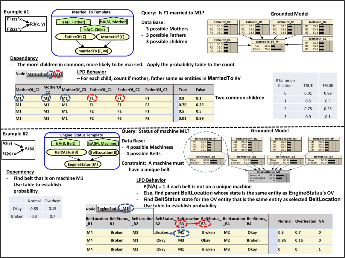
Figure 12 Existential Child Pattern examples—OVs of child RV involved as selectors. Overlaid onto paired or multi-existential behaviors

Example #2 looks like an Existential Paired pattern but has a CSI twist. Here, the problem is to determine the status of a specific machine (M1), based on the status of a cooling fan belt on that machine. There is uncertainty about which belt is on which machine (BeltLocation). There is also uncertainty about the status of each belt. There is a constraint on this problem (the NA in EngineStatus). There must be a unique belt on each machine. In each PC, the LPD looks at the location and status for each belt. Because one is interested only in machine M1, the LPD checks whether the state of BeltLocation matches the OV in the child RV, EngineStatus. This gives the LPD a CSI twist. If the machine is not M1, it is ignored. If it is, then the belt status of the associated belt affects EngineStatus states per the probabilities in the table.

The reader may note that Example # 1 in Figure 6 and Example #2 in Figure 12 have the same basic dependency model, but result in different patterns. This is due to two factors. The first is that they have different variable combination—variables x and y in F2 are inverted. This creates different grounded model structures, which is a basic difference between selector and existential selector patterns. The second factor is that creating the LPD for Example #2 in Figure 12 requires knowledge about what the specific entity of the child RV is.

Although this research focused on single and dual RV-type parents to identify the patterns, many real-world problems require more complex implementations of the patterns. Selection patterns recur widely, especially in PRMs. One can extend the patterns presented here to a multiple RV-type problem. One example is a three RV-type model, where two parent RV-types are used as existential selectors. The original model was developed by Kazemi et al. (Reference Kazemi, Fatemi, Kim, Peng, Tora, Zeng, Dirks and Poole2017). They explored the performance of various aggregators on a common problem. The intent was to understand performance differences, rather than developing the most efficient solution process for the problem. The problem is to determine the gender of a movie rater, given a database of movie ratings given by raters whose gender is known. The template is in Figure 13. This example uses one aggregator they developed, which has a double selection processFootnote ⁹. The database includes entities for Movie and Rater, and has multiple relations and attributes. For this model, two relationships and one attribute are used: GRates, a Boolean relation that states whether a particular rater has rated a specific movie, and Gender, the gender attribute of the rater. The RV Rates(X,M) is used to identify the set of movies the rater being queried about has rated. The context node ~(X = Y) ensures that information about the query entity is not included in the LPD model.

Figure 13 Movie rater gender model

The model is a conditional double count model. For each movie, if rater x has not rated it, it is ignored. Rates(X, M) is the first selector. If rater x has rated it, the second selector guides the counting of both the number of female raters (denominator) and total number of raters (numerator). The probability is

(5)\begin{align} P{\text{(}}Gender\left( x \right) = Female|E) = \frac{c + \sum \nolimits_m [I\left( Rates\left( {x,m} \right) \right){*}\sum \nolimits_{y} \left( I\left( GRates\left( {y,m} \right){*}\ I\,\left( Gender\left( y \right) = F \right) \right) \right]}{{2c + \mathop \sum \nolimits_{m{\text{\;}}} [I\left( {Rates\left( {x,m} \right)} \right){*}\mathop \sum \nolimits_{y{\text{\;}}} I\left( {Rates\left( {y,m} \right)} \right)]}} \end{align}

where m is the set of movies and I is an indicator function with value 1 if the RV instance has state True or if the specified state is true (e.g. Gender = female), else it is 0. The constant c represents a pseudo count as a prior and is established via a learning algorithm prior to using the model.

4.5 Embedded dependency patterns

The third pattern category is Embedded Dependency patterns. These all are single parent-type patterns. There is not a second RV type that enables the linkage between the first RV type and the child RV. This research identified two different embedded dependency patterns: conversion/inversion patterns and existence patterns.

The Conversion pattern switches an F-type RV to an equivalent set of R-type RVs, and vice versa. It is useful when the knowledge base has information in one form, but when the other form is more appropriate for the model. An example of each is shown in Figure 14. The F-to-R conversion is a simplified model converting a functional representation of possible causes of death (assumed to be collectively exhaustive) to a series of relationship RVs, one for each cause. The LPD is guided by the child’s OV. If the state of the parent CauseOfDeath matches the Cause class OV in DeathCausedBy, then the child’s state is True. Otherwise, it is False.

Figure 14 Conversion/Inversion Patterns—changing forms when needed to better fit rest of model/data

In the R-to-F conversion, one is taking a constrained (exactly one) group of relationship RVs and converting them to a single functional F-type RV. The LPD includes an embedded constraint. All PCs with more than one parent true or with no parent true map to the NA state. For remaining PCs, the state of the child is set to the Parent entity that has a state True.

The Inversion pattern provides the inverse of a relationship, which is not necessarily the same relationship with the variable order reversed. For example, hasFriend(x,y) is normally considered a symmetricrelationship and is its own inverse. But hasChild(x,y) and hasParent(y,x) are each an antisymmetric relationship, but are considered inverses of each other. If the inverse of a relationship is a different relationship, the modeler needs to understand the nature of the inversion. The naming of the RVs and determining whether the two RVs have the same semantic meaning is the modeler’s responsibility. The pattern only ensures that the uncertainties among the states are preserved between the RVs. Trivially, one can always create an inverse by switching the voice (active/passive) of the verb phrase that defines the relationship. For example, hasFather(x,y) and isFatherOf(y,x) are formally inverses of each other. But often one is interested in an inverse that describes the relationship differently, such as hasChild(x,y) and hasParent(y,x). In those cases, the dependency between the two may not be as tightly bound.

Because relationships can be expressed either as R-type (always) or F-type (for a functional relationship), there are four possible implementations, as shown in Figure 14. In the F-F case (BeltLocation(b)/m to BeltOn(m)/b), there must be a one-to-one relationship between the entities in the OV and SV of the two RVs. The NA constraint in the child RV enforces this requirement. Note the effect of having this constraint on the grounded model. While the query would be on one entity, the query-specific construction algorithm will instantiate a child RV for each entity in the OV class. This occurs because the finding on each BeltOn RV instance that NA must have zero probability means that each BeltOn instance becomes d-connected to every other BeltOn RV. The LPD is straightforward—the specific belt on a machine is the parent with the same state as the OV of that machine. The LPD includes a count command, which counts the number of instances that meets the criterion between the parentheses.

The R-R case (hasGrandparent(y,x) to hasGrandchild(x,y)) is the most flexible, as it puts the least restrictions on what can be modeled. In the example, the LPD is simply that the probabilities of hasGrandparent(y,x) are the probabilities of hasGrandchild(x,y). In the R–F case, there is a requirement that the R-type parent must be functional for the OV that is also the OV of the child variable (child in the example). If a child has two biological fathers, this violates the mutually exclusive nature of FatherOf. The embedded constraint exists to enforce this requirement. For those PCs that meet the constraint, the LPD looks for which hasChild instance is True and assigns a probability of 1 to the child state that is the same entity as the parent OV. The last case, F–R, is an example where the inverse has additional characteristics. Instead of the grandparent/grandchild inverses, one now has an F-type parent called PaternalGrandfatherOf with an R-type child RV (hasGrandchild). hasGrandchild is not tied so tightly to the parent RV. It is possible for the paternal grandfather to be one person, while the OV in hasGrandchild is true for another person. This is because a human child has two grandfathers, of which one is the paternal grandfather. The LPD table provides a probability for this case.

Existence patterns are single parent patterns that describe dependencies between attributes and relationships. In these patterns, the same entity has both the attribute and the relationship under consideration, and the state of one influences the state of the other. Figure 15 gives three examples. In the first, an attribute (a person’s sex) affects whether that person can be the mother of another person. In the LPD, all male persons have zero probability, while females have a uniform probability whose value depends on their count. In this example, the list of possible mothers is assumed to be complete.

Figure 15 Existence Patterns—dependency based on common meaning between concepts in parent and child RVs

In the second example, a set of relationships BossOf influence whether a manager is a busy person. In this case, the LPD looks at a set of employees and counts if a particular manager is their boss. The higher the count, the higher the degree of busyness. In this example, the states of busyness are a sequence of qualitative levels of busyness, rather than a yes/no assessment. In the third example, an attribute (Personality) influences the likelihood that a person will be friends with another person. The LPD is a straightforward implementation, with conditional probabilities for each of the states of the parents.