I. Introduction
The potential for fine wine to improve with age, along with variable growing conditions each season, means that there has long been an active secondary market for wine (Robinson, Reference Sanning, Shaffer and Sharratt1999). In more recent decades, there has been interest in wine, along with other collectable items such as art, as an alternative asset class. This interest in the financial return available from holding wine has led to the publication of a number of studies that have estimated the return to wine.
The first generation of studies that sought to evaluate the investment potential of wine considered only wine returns, and these studies found mixed evidence regarding the value of wine as an asset class (Burton and Jacobsen, Reference Burton and Jacobsen2001; Fogarty, Reference Fogarty2006; Jaeger, Reference Jaeger1981; Krasker, Reference Krasker1979). A second generation of studies then appeared that also considered the potential of wine to provide a risk diversification benefit if added to an investment portfolio, and these studies all found a low or negative correlation between wine and standard financial assets (Fogarty, Reference Fogarty2010; Masset and Henderson, Reference Masset and Henderson2010; Masset and Weisskopf, Reference Masset, Weisskopf, Giraud-Heraud and Pichery2013; Sanning et al., Reference Sanning, Shaffer and Sharratt2008).
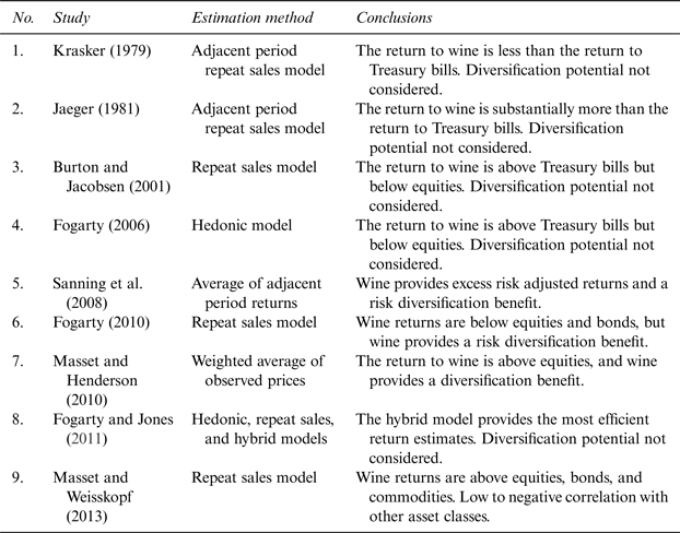
The existing literature on the return to wine is summarized in Table 1. Specifically, for each study that has estimated the return to wine, Table 1 provides information on the approach taken to estimate returns and the conclusions drawn. As can be seen by reading down the estimation method column of the table, the literature has not settled on a standard statistical methodology for estimating the return to wine. The lack of a standard statistical methodology for estimating returns is one factor that contributes to the variation in reported results. Other factors that contribute to the variation in reported results include consideration of different time periods, use of wines from different regions, and the use of sales data from different countries. Our study contributes to the return to wine literature by exploring the impact of estimation methodology on findings.
Table 1 Return to Wine Literature Summary

Note: The return measure considered is the return to the all wine portfolio reported in each study.
We begin our study by outlining six different approaches to estimating the return to infrequently traded heterogeneous assets such as wine, art, and other collectables. This is an expansion of the range of methods considered in Ginsburgh et al. (Reference Ginsburgh, Mei, Moses, Ginsburgh and Throsby2006), where the context was estimation of an art price index. Using Australian wine auction data to illustrate each method, we then show that the choice of estimation method has a significant impact on the estimated return distribution and that, unlike standard financial assets, wine risk and return estimates are sensitive to small changes in the time period considered.
To investigate whether the risk diversification test chosen affects conclusions about wine's potential to lower portfolio risk, a variety of testing approaches are considered. We show that the conclusion drawn about the risk diversification benefit attributable to wine depends on: (i) the method used to estimate the return to wine; (ii) the diversification benefit testing approach selected; (iii) the time period considered; and (iv) whether the analysis is conducted in terms of excess returns or raw returns.
II. Return to Wine Estimation Methods
In general, academic economists have favored regression-based methods to estimate the return to wine. From the auction house perspective, regression-based approaches to estimating the return to wine have several drawbacks, the most prominent of which is that after each auction the entire index needs to be re-estimated, and, hence, after each auction there are revisions to historical estimates of the return to wine. For this reason, and the fact that the regression methodology is not widely understood by the general public, auction houses generally rely on non–regression-based approaches to estimate the return to wine. Here, four regression-based approaches and two non–regression-based approaches that are relevant to the wine investment literature are considered.
A. The Hedonic Model
Regression model 1 is the hedonic model. As detailed in Triplet (Reference Triplett2004), the hedonic approach has a long history. The approach can be understood as follows. Let the time of sale be indexed by t (t = 0, . . . , T), and let the set of all observed wine sales at auction be indexed by w (w = 1, . . . , W) so that P wt denotes the price of wine w sold at time t and p wt denotes the log price of wine w sold at time t. Now, let each bottle of wine in the sample be described by the attribute set {x k} (k = 1, . . . K). With this notation, the hedonic model can be written as:
where d wt is a dummy variable that takes the value of 1 if wine w was sold at time t, and 0 otherwise. In equation (1), the error term εwt comprises a random component and possibly a time-independent specification error component. If there is a time-independent specification error component, it is assumed to be uncorrelated with the x k. The hedonic model can be estimated using least squares, with the period-by-period returns calculated from the γt estimates. A key advantage of the hedonic approach is that it uses all available sales observations. A significant drawback of the approach is that if the hedonic model is misspecified, the estimates of price change are biased (Benkard and Bajari, Reference Benkard and Bajari2005).
B. The Repeat Sales Model
Regression model 2 is the repeat sales model as in Bailey et al. (Reference Bailey, Muth and Nourse1963), and the approach can be understood as follows. Of the set of all wines sold, a subset will sell on more than one occasion. Let the set of wines that sell more than once be indexed by j, and for wine j let the first sale take place in period t and the second sale take place in period τ, where τ > t. Now, for these repeat sale wines, rewrite equation (1) with the first sale and second sale observations identified separately:
The repeat sales model is found by subtracting (2a) from (2b) to give:
where D jτ takes the value 1 if wine j was sold in period τ, –1 if wine j was sold in period t, and 0 otherwise. As with the hedonic model, the return to wine is calculated from the estimates of γt. Unlike in the hedonic model, there is no potential misspecification problem when only repeat sales are used. However, the approach does not use all available sales information. Further, as higher quality vintages trade more frequently (Ashenfelter et al., Reference Ashenfelter, Ashmore and Lalonde1995), there is a potential sample selection problem with this approach.
C. The Pooled Model
Regression model 3 is the pooled model, where the name is due to the model representing a “pooling” of the hedonic and the repeat sales models. The pooled model has not been used previously to estimate the return to wine. It is an approach that is similar to the hybrid model but much simpler to implement. The approach can be understood as follows. Let the wines that are sold only once be indexed by i, and again let the repeat sale observations be indexed by j. Now, rewrite equation (1) for the full set of wine sale observations, such that the single sales, as well as the first and second repeat sales, are identified separately:
Differencing equation (3b) from equation (3c) gives the repeat sales model:
and the pooled model is estimated as equations (3a), (3b), and (3d) stacked in that order. As the approach uses all the data, the pooled model could be seen as an improvement on the repeat sales model. Note, however, that the model does not address the potential misspecification problem that arises when using hedonic models.
D. The Hybrid Model
Regression model 4 is the hybrid model used in Case and Quigley (Reference Case and Quigley1991), where the specific implementation of the approach presented here follows Fogarty and Jones (Reference Fogarty and Jones2011). The hybrid model can be developed as an extension of the pooled model, where the extension relates to how the error term is treated. As presented here, the hybrid model error term εwt is decomposed into a zero mean constant variance pure random error term denoted e wt, and a zero mean constant variance time independent specification error term denoted ηw. This decomposition of the error term into two parts means that following the same steps as for the pooled model, the hybrid model can be written as:
The model assumptions then follow those of a random effects panel model and are: E(η w) = E(e wt) = 0, Var(η w) = σ η2, Var(e wt) = σ e2, and Cov(e it, ejt) = Cov(e wt, ewτ) = Cov(e wt, ηw) = 0 and Var(ε wt) = σ e2 + σ η2. These assumptions then give rise to a model with covariance matrix structure:
 $${\bf \Omega}_1 = \left[ {\matrix{ {\sigma_{\varepsilon}^2 {\bf I}} & {\bf 0} & {\bf 0} \cr {\bf 0} & {\sigma _\varepsilon ^2 {\bf I}} & { - \sigma _e^2 {\bf I}} \cr {\bf 0} & { - \sigma _e^2 {\bf I}} & {2\sigma _e^2 {\bf I}} \cr}} \right].$$
Relying on the random effects panel model analogy, and the need for consistent estimates of the elements of ![]() ${\bf \Omega} _1 $$ only, Jones (2010) proposes using the errors from equation (1) to obtain a consistent estimate of σ ε2 as
${\bf \Omega} _1 $$ only, Jones (2010) proposes using the errors from equation (1) to obtain a consistent estimate of σ ε2 as ![]() $\hat{\sigma}_\varepsilon ^2 = \left( {\displaystyle{1 \over {W - K - 1}}} \right)\mathop \sum \nolimits_{w = 1}^W \hat{\varepsilon}_{wt}^2 $ and using the errors from equation (2c) to obtain a consistent estimate of σ e2as
$\hat{\sigma}_\varepsilon ^2 = \left( {\displaystyle{1 \over {W - K - 1}}} \right)\mathop \sum \nolimits_{w = 1}^W \hat{\varepsilon}_{wt}^2 $ and using the errors from equation (2c) to obtain a consistent estimate of σ e2as ![]() $\hat{\sigma}_e^2 = \displaystyle{1 \over 2}\left( {\displaystyle{1 \over {J - T}}} \right)\mathop \sum \nolimits_{j = 1}^J \left( {\hat{\varepsilon}_{j\tau} - \hat{\varepsilon}_{jt}} \right)^2 $. With equations (4a), (4b), and (4c) stacked in that order, and y and X used to denote, respectively, the stacked column vector of prices and price differences, and the design matrix; the method of Feasible Generalized Least Squares can then be used to estimate the time index and other attribute implicit prices via direct multiplication as
$\hat{\sigma}_e^2 = \displaystyle{1 \over 2}\left( {\displaystyle{1 \over {J - T}}} \right)\mathop \sum \nolimits_{j = 1}^J \left( {\hat{\varepsilon}_{j\tau} - \hat{\varepsilon}_{jt}} \right)^2 $. With equations (4a), (4b), and (4c) stacked in that order, and y and X used to denote, respectively, the stacked column vector of prices and price differences, and the design matrix; the method of Feasible Generalized Least Squares can then be used to estimate the time index and other attribute implicit prices via direct multiplication as ![]() $\left({\bi X}^{\bf \prime} \hat{\bf \Omega}_1^{ \bf- 1} {\bi X} \right)^{\bf- 1} {\bi X}^{\bf \prime} \hat{\bf \Omega}_1^{ \bf- 1} {\bi y}$. In practice, finding
$\left({\bi X}^{\bf \prime} \hat{\bf \Omega}_1^{ \bf- 1} {\bi X} \right)^{\bf- 1} {\bi X}^{\bf \prime} \hat{\bf \Omega}_1^{ \bf- 1} {\bi y}$. In practice, finding ![]() $\hat{\bf \Omega} _1^{ - 1} $ directly is impractical for data sets of moderate size; and even if it were possible to find
$\hat{\bf \Omega} _1^{ - 1} $ directly is impractical for data sets of moderate size; and even if it were possible to find ![]() $\hat{\bf \Omega} _1^{ - 1} $ directly, the subsequent direct application of the FGLS multiplication process is likely to be unstable. To estimate the model Fogarty and Jones (2011) suggest taking advantage of the block diagonal structure of
$\hat{\bf \Omega} _1^{ - 1} $ directly, the subsequent direct application of the FGLS multiplication process is likely to be unstable. To estimate the model Fogarty and Jones (2011) suggest taking advantage of the block diagonal structure of ![]() $\hat{\bf \Omega} _1 $. Specifically, the authors suggest creating a matrix, say
$\hat{\bf \Omega} _1 $. Specifically, the authors suggest creating a matrix, say ![]() $\bar{\bf \Omega}_1 $, that is a proportionally much small version of
$\bar{\bf \Omega}_1 $, that is a proportionally much small version of ![]() $\hat{\bf \Omega} _1 $. For this relatively small matrix, the Cholesky decomposition can be used to find
$\hat{\bf \Omega} _1 $. For this relatively small matrix, the Cholesky decomposition can be used to find ![]() $\bar{\bi P}$, such that
$\bar{\bi P}$, such that ![]() $\bar{\bi P}^{\prime} \bar{\bi P} = \bar{\bf \Omega}_1^{ - 1} $. It is then possible to scale
$\bar{\bi P}^{\prime} \bar{\bi P} = \bar{\bf \Omega}_1^{ - 1} $. It is then possible to scale ![]() $\bar{\bi P}$ up to the full-size matrix P, such that
$\bar{\bi P}$ up to the full-size matrix P, such that ![]() ${\bi P}^{\bf \prime}{\bi P} = \hat{\bf \Omega}_1^{-1}$. The full-size P matrix can then be used to pre-multiply y and X, to give y * and X *. Estimates of the time index and the attribute implicit prices are then obtained using OLS on the transformed data (X *′X *)−1X*′y *. An important aspect of this approach is that it relies on the very robust routines used for least squares estimation implemented in standard software packages.
${\bi P}^{\bf \prime}{\bi P} = \hat{\bf \Omega}_1^{-1}$. The full-size P matrix can then be used to pre-multiply y and X, to give y * and X *. Estimates of the time index and the attribute implicit prices are then obtained using OLS on the transformed data (X *′X *)−1X*′y *. An important aspect of this approach is that it relies on the very robust routines used for least squares estimation implemented in standard software packages.
The hybrid model is currently the most comprehensive regression-based approach to estimating returns, and this is its strength. The main disadvantage of the approach is that estimation is relatively complex.
E. The Average Adjacent Period Return Model
The first non–regression-based approach considered is the average adjacent period return model, and if h is used to index the set of wines with adjacent period sales, the model can be written as:
where r t+1 is the return to wine for period t + 1. The approach is simple to implement and understand but excludes a large proportion of the available information. To the extent that better vintages trade more frequently, the approach will overstate the return to wine.
F. Commercial Index Model
The final model considered is based on the method used by the Australian wine auction house Langton's. The method may be understood as follows. Let P lt denote the price of wine l sold at time t. If wine l is sold at time t + 1 then the price observation is updated. If wine l is not sold at time t + 1 then P lt+1 = P lt. Letting ![]() $\bar P_t = \mathop \sum \nolimits_{l = 1}^L P_{lt} $, the market return to wine at time t + 1 is found as:
$\bar P_t = \mathop \sum \nolimits_{l = 1}^L P_{lt} $, the market return to wine at time t + 1 is found as:
Although the approach is simple to implement and understand, the assumption that if a wine did not sell in a given period, the price it would have sold for is the price in the previous period is strong. In practice, the assumption means that the approach is likely to understate the risk associated with wine investment. That the variance of returns is understated, is, however, a criticism that could also be leveled at all regression-based approaches.
III. Data and Return Estimate Comparison
In any study tracking the performance of wine, it is necessary to be clear regarding the wines included in the sample. Globally, almost all the wine sold is not produced with extended aging in mind. For example, in Australia, around 99.5 percent of domestically produced and sold wine retails for less than US$26 per bottle (WFA, 2013),Footnote 1 and most of this wine is ready for consumption at the time of purchase. Wine investors are not interested in the return to the average retail bottle of wine but wines that will benefit from extended aging. We therefore restrict the sample of wines to wines classified as investment grade wines in the Caillard and Langton (Reference Caillard and Langton2001) guide to wine investment in Australia. There are also very rare, very old wines that trade infrequently. Due to their rarity, these wines trade more as antiques than investment wines, and these wines are excluded from the study. Specifically, wines more than 35 years old were excluded from the study. For another context, say wines from Bordeaux, the definition of old and rare wines might be different.
The dataset used to investigate the impact of estimation method on the wine return distribution consists of 14,102 sale observations on investment grade Australian fine wine sold in Melbourne and Sydney by the Australian auction house Langton's, over the period 1988Q1 to 2000Q4. Although it would be valuable to consider a more recent sample period, it has not been possible to construct a longer time series using consistent data sources. The specific wine brands in the sample and the main grape variety used in each wine brand are listed in the appendix. The majority of observations in the sample (87 percent) are for red wines.
In terms of the hedonic model, the attributes that are assumed to describe the sale price of a bottle of wine are: the wine brand (84 individual brands), the wine vintage (years 1965 to 2000), and the time of sale (1988Q1–2000Q4). As such, the specific form equation (1) takes is:
where the βk control for brand differences, the θv control for vintage differences, and the γt give a log index of the return to wine.
A. Impact of Estimation Method
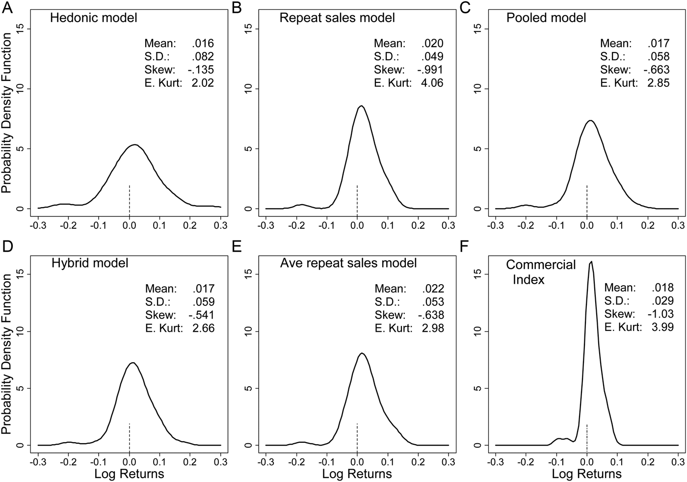
The first research objective is to understand the impact of the estimation method on the wine return distribution. To answer this question, Figure 1 presents kernel density estimates and summary information on the return distribution using the six different estimation methods considered. From Figure 1, and the summary information that has been added to each plot, it is clear that the estimation method has a material impact on the implied return distribution. The excess return distribution was also calculated by subtracting the return available at the start of each quarter from holding 90-day Treasury bills. However, as the key findings based on the excess return information are the same as those based on the raw return information, the excess return information is not discussed.

Figure 1 Wine Log Return Distribution Plots: 1988Q1–2000Q4
Across the six estimation approaches, the method with the most attractive theoretical properties is the hybrid approach, and in the remaining discussion the hybrid estimates are considered the reference estimates. For the first moment of the distribution, it can be seen that the hedonic method provides the lowest estimate and the average adjacent period method the highest estimate; the difference is material: 1.64 percent versus 2.23 percent. The commercial index approach, in which wines are held at their last sale value until they sell again, appears to result in a modest upward bias in the mean return estimate.
Across the estimation methods, the observed pattern in the mean return estimates has an intuitive explanation. As previously noted, the best wines, in the sense that their price growth is fasted, are traded most frequently. The method most susceptible to capturing this bias is the average adjacent period method, followed by the repeat sales method. These methods, therefore, generate overly optimistic return to wine estimates. This result is also consistent with findings from the art market that suggest the repeat sales model is likely to be inappropriate for time frames of less than 20 years (Ginsburgh et al., Reference Ginsburgh, Mei, Moses, Ginsburgh and Throsby2006).
Model misspecification, and hence biased return estimates, is a potential problem for all hedonic models. Previous work has, however, shown that return estimates from deliberately misspecified art index hedonic models can still be quite accurate (Ginsburgh et al., Reference Ginsburgh, Mei, Moses, Ginsburgh and Throsby2006). Here, the difference in the mean quarterly return estimate between the hedonic approach and the hybrid approach is 0.07 percentage points. One interpretation of this result could be that for Australian wine, the relevant attributes are quite clear, and so the potential for misspecification error is relatively small.
For practical purposes, the mean return to wine estimate from the pooled model and the hybrid model are identical. Given that estimation of the hybrid model is substantially more difficult than estimation of the pooled model, this suggests that if one is only interested in the mean return to wine, there is no need to use the more complex hybrid model. Note, however, that the motivation for implementing a hybrid type model is generally that the approach results in smaller standard errors for the price index point estimates. Here we found that the hybrid approach resulted in the smallest average standard errors around the price change point estimates. Specifically, the average standard error surrounding each point estimate of price change for the four regression based models was: hedonic model .0427, repeat sales model .0533, pooled model .0403, and hybrid model .0325.
For the second moment of the distribution, Figure 1 shows that the commercial index approach substantially understates the risk associated with wine investment. For the commercial index approach, the standard deviation of returns is 2.99 percent, while for the hybrid method it is 6.04 percent. For the second moment of the distribution, another notable result is that the hedonic method appears to significantly overstate the risk of wine investment (8.85 percent). It is also notable that, as in the findings for the mean return estimates, the standard deviations found by using the pooled model and the hybrid model are essentially the same.
Given the length of the sample, and the fact that investors generally consider only the first two moments of the distribution, the intention here is not to overstate the differences observed for the higher-order moments. It is, however, notable that the estimates for the third and fourth moments of the distribution obtained for the pooled model and the hybrid model are very similar.
In summary, the evidence suggests that the method used to estimate the return to wine has a material impact on the estimated return distribution. As in the art market (Ashenfelter and Graddy, Reference Ashenfelter, Graddy, Ginsburgh and Throsby2006, 916–917), repeat sale approaches overstate returns in the wine market. The commercial index approach has a modest upward bias in the mean return estimate but substantially understates risk. The hedonic, hybrid, and pooled models all give similar mean return estimates. So, if the analysis concerns only the first moment of the distribution, any of these methods could be considered appropriate. The hedonic model did, however, overstate risk, and, so, for analysis that relies on both the first and second moment of the distribution, the pooled model or the hybrid model would be more appropriate.
B. Impact of Changes in the Sample Period
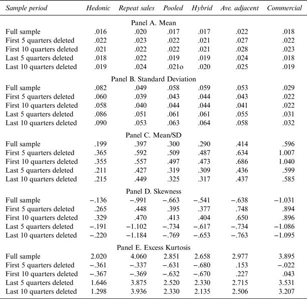
The second research objective is to understand the impact of relatively small changes in the period under consideration on the return distribution. It seems appropriate that for all classes of alternative assets, such as art, antiques, wine, and other collectables, return information should be calculated to the most recent date possible. It is, however, much less clear that, for any given asset class, there is a specific, objective, reference sample start date. If small changes in the sample start date have a material impact on the return distribution, investors need to be cautious in how they interpret alternative asset return information. Given the length of the sample available, the extent of sensitivity testing regarding the effect of sample period is necessarily limited but still provides useful insights. Specifically, to understand the impact of small changes in the sample period, the first and last five and ten quarters of the sample were sequentially dropped, and key metrics calculated for each subperiod. This information, along with information for the full sample period, is shown in Table 2.
Table 2 Wine Return Characteristics: Quarterly Log Returns

In each panel of Table 2, the first row contains the information calculated for the entire sample, and the remaining rows contain information for the subsamples. The first panel of Table 2 shows that, regardless of estimation method, small changes in the sample period can have a significant impact on the mean return estimate. Across the six estimation methods, dropping the first five quarters of the sample results in an increase in the mean quarterly return of around half a percentage point. Small changes in the sample have a similarly large impact on the other moments of the distribution. Panel C of Table 2 contains information on the return per unit of risk. For this metric, dropping observations at the end of the sample appears to have a relatively modest impact. Dropping observations at the start of the sample period, does, however, result in substantial changes to the metric.
C. Estimation Method and Sample Period Summary
Taken collectively, the information presented in Figure 1 and Table 2 suggests the following. First, the wine return distribution varies substantially with the estimation method. Second, across all wine return estimation methods, relatively small changes in the period under consideration have a substantial impact on the risk, return, and risk-adjusted return estimates. Third, the return distribution obtained using the commercial index approach is strikingly different from the one obtained for all other estimation methods. Fourth, as in the art market, repeat sales models overstate the return to wine.
In terms of the most appropriate estimation approach to use for index construction, the pooled model appears to strike the right balance between index accuracy and ease of implementation. For these reasons, the pooled model, rather than the repeat sales model that has been the most commonly used approach to date, is our preferred approach for estimating the return to wine.
IV. Risk Diversification Benefit Tests
A number of different approaches can be used to test for a risk diversification benefit, and it is valuable to understand whether findings regarding the impact of adding wine to an investment portfolio vary with the testing method used. Although most applied financial analysis relies on excess return data, in some cases, such as Jobson (Reference Jobson1982), the risk-free rate is assumed to be zero. Some studies in the existing return to wine literature, such as Fogarty (Reference Fogarty2010), also use raw returns to test for a risk diversification benefit. As such, here, both raw return and excess return data are used. Additionally, as the return analysis showed that the return distribution can vary significantly with small changes in the sample period, for each risk diversification benefit test, the analysis is undertaken using: (i) the full data set; (ii) the full data set minus the first five quarters; and (iii) the full data set minus the last five quarters.
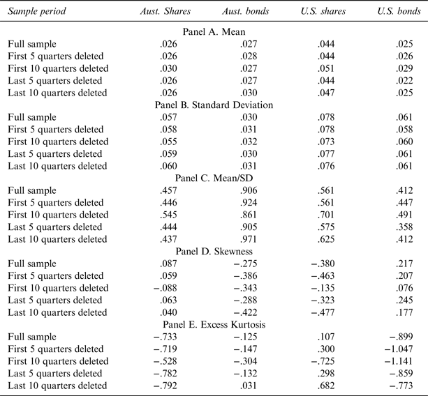
The return information for standard financial assets was obtained from Datastream, and it can be noted that for U.S. equities the returns are total returns for the S&P 500, and for Australian equities, returns are total returns for the All Ordinaries Index. Both the Australian and U.S. bond return information relates to the relevant JPMorgan index series. For both U.S. bonds and U.S. equities. the returns are unhedged Australian dollar returns. The standard financial asset information is summarized in Table 3. To allow for a comparison with the return to wine information, Table 3 has the same format as Table 2. As can be seen, and in contrast to the wine return information, for the standard financial assets considered, small changes in the sample period have little impact on the return distribution.
Table 3 Standard Financial Assets: Quarterly Log Returns

The diversification benefit discussion is grouped into two sections. The first section considers approaches that use a single metric to determine whether adding wine to an investment portfolio provides a diversification benefit. The second approach is a relatively novel approach that relies on a visual display of information. Specifically, the approach plots the change in the efficient frontier when wine is added to an investment portfolio, along with confidence intervals. This approach gives a measure of the practical effect of adding wine to different types of efficient investment portfolio.
A. Single Metric Diversification Benefit Tests
The first approach used to test for a diversification benefit is based on Jobson (Reference Jobson1982). The Jobson approach uses an F-test to compare the performance of a portfolio containing a subset of assets against the full portfolio. Within the Jobson framework, a portfolio is said to be market efficient if the ratio μ2/σ2 is maximized, where μ denotes portfolio return and σ2 denotes portfolio variance. If u is used to denote the mean return vector for the full set of assets, and V is used to denote the associated sample covariance matrix, under conditions of no short selling and a fully invested portfolio, the maximum value of the ratio μ2/σ2 is given by u′V –1u. If u r and V r are used to denote, respectively, the mean return vector and the sample covariance matrix for the restricted portfolio containing only a subset of assets, the Jobson test can be understood as a test of the hypothesis that u′V –1u = u r′Vr− 1u r.
Following Jobson (Reference Jobson1982), the test is implemented as an F-test, and summary test information is provided in Panel A of Table 4. In the table, the values are the F-test p-values. A low p-value indicates that it is possible to reject the null hypothesis of no portfolio performance improvement following the addition of wine to the portfolio with relative confidence.
Table 4 Summary Results for Single Metric Diversification Benefit Tests

Note: For the results in Panel B, in each case the correlation to an equally weighted portfolio of standard financial assets is never statistically different from zero. Assuming the correlation coefficient is zero leaves unchanged the key result that conclusions about the diversification benefit of wine are sensitive to: the use of raw returns versus excess returns, the return to wine estimation method selected, and the period considered.
The second approach used to test for a diversification benefit is based on an approach outlined in both Blume (Reference Blume1984) and Elton et al. (Reference Elton, Gruber and Rentzler1987). In this application, we use the approach to test whether there is a diversification benefit from adding wine to a portfolio consisting of an equally weighted portfolio of the four standard assets identified in Table 3. Under this testing approach, the portfolio investment objective is to maximize return per unit of risk, and following the Elton et al. (Reference Elton, Gruber and Rentzler1987) form of the test, if the return per unit of risk for wine (r w/σw) is greater than the return per unit of risk for the existing market portfolio multiplied by the correlation coefficient between the portfolio and wine (r p/σp) ρwp, there is a diversification benefit from adding wine to the market portfolio. This decision rule follows from the conditions for the inclusion of an asset in the optimal portfolio established in Elton et al. (Reference Elton, Gruber and Padberg1976). The specific test values reported in Panel B of Table 4 are (r w/σw) − (r p/σp) ρwp. This means that a positive value in the table indicates a diversification benefit from adding wine to the portfolio, and a negative value indicates no diversification benefit.
The third approach to testing for a risk diversification benefit is the mean-variance spanning approach. When considering the addition of a single asset class to an existing investment portfolio, an appropriate mean-variance spanning test is the Huberman and Kandel (Reference Huberman and Kandel1987) regression based test. In this instance, the test involves regressing the return to wine from each estimation method on the return to the assets already in the investment portfolio and an intercept term. In such a regression, if the intercept is zero, and the sum of the point estimates on the other asset classes is one, the conclusion drawn is that the return to wine can be synthetically reproduced by a weighted sum of the assets already in the investment portfolio, and the return to wine is said to be spanned by the existing assets. If the return to the test asset can be synthetically reproduced by the assets already in the investment portfolio, the test asset has no value to the portfolio.
The form of the spanning test regression is ![]() $\ddot r_{jt} = \alpha + \mathop \sum \nolimits_{i = 1}^K \beta _i r_{it} + u_{jt} $, where
$\ddot r_{jt} = \alpha + \mathop \sum \nolimits_{i = 1}^K \beta _i r_{it} + u_{jt} $, where
![]() $\ddot r_{jt} $ denotes the return to wine from estimation method j at time t; r it denotes the return to benchmark asset i at time t, and u jt denotes a zero mean constant variance error term. The joint constraint that
$\ddot r_{jt} $ denotes the return to wine from estimation method j at time t; r it denotes the return to benchmark asset i at time t, and u jt denotes a zero mean constant variance error term. The joint constraint that ![]() $\mathop \sum \nolimits_{i = 1}^K \beta = 1$ and α = 0 is then imposed via a Wald test. Panel C of Table 4 reports p-values for tests of the joint restriction that the intercept is zero and the βi sum to one. With low p-values, we reject the null of mean variance-spanning with confidence.
$\mathop \sum \nolimits_{i = 1}^K \beta = 1$ and α = 0 is then imposed via a Wald test. Panel C of Table 4 reports p-values for tests of the joint restriction that the intercept is zero and the βi sum to one. With low p-values, we reject the null of mean variance-spanning with confidence.
Reviewing the three sets of test results in Table 4 reveals some general patterns. First, across the various changes in the period and estimation method considered, the results for the Jobson test are the least stable, and the results for the Huberman and Kandel test are the most stable. Second, evidence in favor of a diversification benefit is generally stronger when raw return data rather than excess return data are used, although the difference is most pronounced with the Jobson test and least pronounced with the Huberman and Kandel test. Third, at a practical interpretation of results level, different conclusions will be drawn about the diversification benefit of wine depending on the type of test used, the sample period considered, and the method used to estimate returns.
B. Mean-Variance Efficient Frontier Plots
The final approach to investigating the potential of wine to provide a risk diversification benefit is the direct estimation of the mean-variance efficient frontier under conditions of no short selling and a fully invested portfolio. The base case results presented represent the classic Markowitz (Reference Markowitz1952) model, where the sample covariance matrix V and the mean return vector u are used in the optimization model.
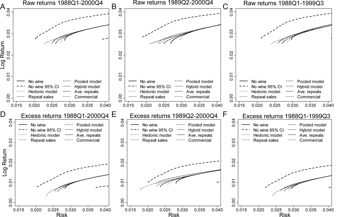
The results of this approach are summarized in Figure 2, and the process for generating the plots can be understood as follows. First, for the three periods considered, we derive the efficient frontier using both raw return data and excess return data, with the allocation to wine restricted to zero. These six efficient frontiers were then plotted in risk-return space. For each of the six scenarios considered, we then construct a 95 percent confidence interval via circular block bootstrapping to account for time-series dependence in the asset returns (Politis and Romano, Reference Politis, Romano, LePage and Billard1992). Here we chose a block size that is optimal for constructing a confidence interval for the Sharpe ratio, using the method of Ledoit and Wolf (Reference Ledoit and Wolf2008). This optimal block size for the Sharpe ratio was then applied to the data to generate the block bootstrap samples for computing confidence intervals on the efficient frontier.

Figure 2 Statistical Significance of the Shift in the Efficient Frontier: Markowitz Model
Finally, using both raw return and excess return data, for each return to wine series by period combination, we derive the efficient frontier where a positive allocation to wine was allowed. These efficient frontiers were then added to each plot. If there are efficient portfolios with a positive allocation to wine that achieve the same level of return as a no-wine portfolio but have lower risk, wine is said to provide a risk diversification benefit. If the expansion of the efficient frontier extends beyond the 95 percent bootstrap confidence bound, the benefit is said to be statistically significant.
As can be seen from the plots, in all cases a positive allocation to wine allows the efficient frontier to shift to the left; although in most case the shift is quite small. The potential benefit to holding wine is also found to be for portfolios near the global minimum-variance portfolio. The potential diversification benefit to holding wine, is, however, almost always not statistically significant. More generally, the plots convey the message that the diversification benefit from holding wine is not something that could be considered of great practical significance in overall portfolio management.
C. Efficient Frontier Sensitivity Analysis
Many modifications to the classic Markowitz approach to deriving the efficient frontier have been proposed. Here, three impacts are explored : (i) using a shrinkage estimator for the mean return vector; (ii) using a shrinkage estimator for the covariance matrix; and (iii) considering higher-order moments. In the analysis, the main element of interest is the allocation to wine in efficient portfolios.
The first scenario we consider is the use of a shrinkage estimator for the mean return vector. Specifically, the Jorion (Reference Jorion1985) return vector is calculated as r = αü + (1 − α)u, where ü is a vector with all elements equal to the return of the global minimum-variance portfolio, u is the mean return vector, and the weights α are determined by the data. As a practical matter, it can be noted that the weight given to ü increases the closer ü is to u.
The second scenario considered is the use of a shrinkage estimator for the covariance matrix. Specifically, the Ledoit and Wolf (Reference Ledoit and Wolf2004) shrinkage covariance matrix is found as ![]() $\ddot {\bi V} = \displaystyle{k \over T}{\bi F} + \left({1 - \displaystyle{k \over T}} \right){\bi V}$, where F is the single-index model covariance matrix of Sharpe (Reference Sharpe1963), T is the length of the time series, and k is the shrinkage constant. As in Jorion's approach for the mean return vector, the shrinkage constant, and hence the weights, are determined by the data. It can be noted that the shrinkage constant, and hence weight to F, increases with error in the sample covariance matrix and decreases with misspecification error in the single index model (Ledoit and Wolf, Reference Ledoit and Wolf2004).
$\ddot {\bi V} = \displaystyle{k \over T}{\bi F} + \left({1 - \displaystyle{k \over T}} \right){\bi V}$, where F is the single-index model covariance matrix of Sharpe (Reference Sharpe1963), T is the length of the time series, and k is the shrinkage constant. As in Jorion's approach for the mean return vector, the shrinkage constant, and hence the weights, are determined by the data. It can be noted that the shrinkage constant, and hence weight to F, increases with error in the sample covariance matrix and decreases with misspecification error in the single index model (Ledoit and Wolf, Reference Ledoit and Wolf2004).
The impact on the allocation to wine in efficient portfolios when the mean return vector and the covariance matrix are replaced with shrinkage estimators is illustrated in Figure 3. Specifically, Figure 3 plots the weight to wine in efficient portfolios calculated using the Markowitz method, the Jorion method, and the Lediot and Wolf method. The figure shows that, regardless of changes in the method used to estimate the covariance matrix and mean return vector, there is still a range of portfolios with a positive allocation to wine for all methods of calculating the return to wine.

Figure 3 Impact of Using Shrinkage Estimators on Portfolio Attributes
For the sample data, use of the Ledoit and Wolf covariance matrix has little impact on the weight to wine in efficient portfolios. The reason for the lower weight to wine in efficient portfolios when using the Jorion mean return vector can be understood as follows. The practical effect of the Jorion estimator is to reduce the estimate of the expected return available from the best-performing asset classes and increase the estimate of the expected return available from the worst-performing asset classes. The rank order of asset performance is, however, unchanged; hence wine is still always the asset with the lowest return. As such, to achieve a given level of portfolio return, a higher proportion of the total portfolio must be allocated to nonwine assets.
The final aspect considered as part of the sensitivity analysis is whether the inclusion of higher-order moments in the optimization problem affects the allocation to wine in efficient portfolios. The specific question of interest is whether considering higher-order moments would cause the allocation to wine in optimal portfolios to fall to zero. To explore this issue, we used insights from Lai et al. (Reference Lai, Yu and Wang2006) to estimate mean-skew and mean-kurtosis optimal portfolios. Unfortunately, it proved difficult to obtain stable results for these models. Our results suggested that consideration of higher-order moments is unlikely to drive the allocation to wine in efficient portfolios to zero, but we cannot present robust evidence on this point.
V. Conclusions
In the return to wine literature, a variety of statistical methods have been used to estimate the return to wine, among which variations on the repeat sales method have been popular. Our findings suggest that, as with art, the return to wine is overstated when using the repeat sales method, but the hedonic method works quite well. For analysis that considers more than just the first moment of the distribution, a simple extension to the hedonic method is proposed, that, at least in the context of a wine index, seems to add value with little additional cost in terms of estimation complexity.
A range of approaches to testing for a diversification benefit from holding wine were considered. Conclusions about the diversification benefit of holding wine were found to be sensitive to: (i) the method used to estimate the return to wine; (ii) the period considered; (iii) whether raw return data or excess return data are used; and (iv) the type of diversification test. The most transparent approach to testing for a risk diversification benefit from holding wine, or other alternative assets, is the direct estimation of the efficient frontier with bootstrapped confidence intervals. The advantage of this method over the other methods is that, rather than just answering the question of whether there is a diversification benefit, the method is able to put the size of the benefit into context. In this study, the method was able to illustrate that any diversification benefit from holding wine is small and applicable only to portfolios close to the global minimum-variance portfolio.
The adoption of a standard statistical methodology for estimating the return to wine would eliminate one factor that has contributed to the variation in results reported in the return to wine literature. With a consistent approach to estimation methodology, further work that considers longer periods and wine from countries other than Australia would provide valuable insights into the nature of the return to wine and the sources of variation in the return to wine.
Appendix
Appendix Table 1 Specific Wine Brands that Appear in the Sample

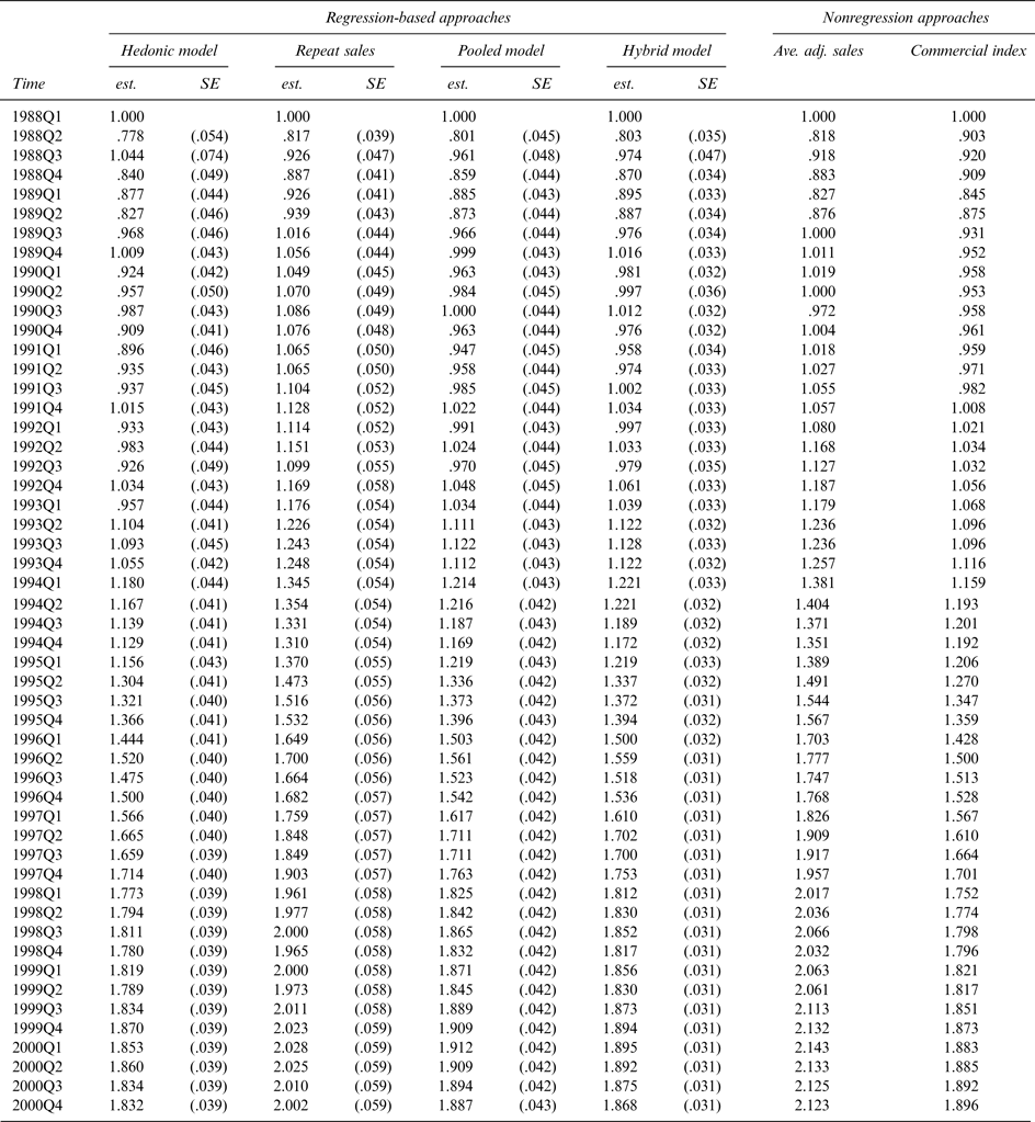
Appendix Table 2 Complete Model Estimation Results: 1988Q1–2000Q4


