


I. Introduction
Wine has traditionally been a symbol of “high class” in China, but it is becoming a regular consumption commodity for a growing middle class (Muhammad et al., Reference Muhammad, Leister, McPhail and Chen2014). By value, China is currently the fourth largest wine importing country in the world (fifth in terms of volume), and it is expected to become the second biggest importer by 2020 (Wine Institute, Reference Institute2017). In the Chinese market, France has a share of approximately 40% overall (and more than 50% for bottled wine sales). China is France's third largest wine export market by value (after the United States and Germany) and the number one export destination for Bordeaux wines.
In this context, the trade relationship between France and China in the wine market is of particular interest. The growing demand for diversity by Chinese customers in recent years, paired with the great variety of French wines, offers a unique opportunity to explore how different French wine regions fare in terms of export performance to China.Footnote 1 Using country and time variation, recent papers have investigated how the exports of different countries responded to the fast growth of gross domestic product (GDP) in China as well as other changes in export determinants (Muhammad et al., Reference Muhammad, Leister, McPhail and Chen2014; Song and Liu, Reference Song and Liu2017). In this article, I focus on within-country regional competition of various French wine regions and their exports to China.
I exploit a dataset on wine shipments of 100 different types of French wines to China between 1998 and 2015. This study treats the wine regions of France as independent exporters in a trade model depending on standard factors such as income (measured by GDP), price (proxied by unit values), exchange rate, and tariffs. This corresponds to a simple demand model that can be estimated using time variation, and that allows retrieving heterogeneous income and price effects across French regions. The approach is similar to the demand analysis based on country and time variation (Muhammad et al., Reference Muhammad, Leister, McPhail and Chen2014; Song and Liu, Reference Song and Liu2017); prices vary over time and country/region while income, proxied by Chinese GDP, varies only over time.Footnote 2
My results first suggest that controlling for time trends is enough to make key variables like log GDP stationary, which is also cointegrated with the log of exported volumes. Overall income and price effects are consistent with the literature based on cross-country variation. Focusing on regional heterogeneity in income and price effects, I suggest that Bordeaux wines remain China's favorite over the period, while regions such as Languedoc and the Rhône Valley are gaining recognition along with a similarly high marginal willingness to pay. Price elasticity is particularly low for highly-reputed wines (Bordeaux and Bourgogne), but it is higher for wines targeted at middle-class customers and from regions traditionally known for white wine. This is consistent with the fact that China mainly consumes red wine. Estimations on a sub-period provide a good out-of-sample fit. A simple forecast model for the years 2019–2022 allows quantifying the impact of reasonable GDP growth prospects for China on its imports of different types of French wines.
This article is structured as follows. Section II presents literature on the determinants of global wine trade and on Chinese wine imports. Section III describes the data and the empirical approach. Results are discussed in Section IV, while Section V presents the conclusion.
II. Related Literature
Wine has long been a part of gift-giving traditions, as well as an indication of social status in China (Liu and McCarthy, Reference Liu, McCarthy, Capitello, Charters, Menival and Yuan2016). The rise in wine imports and consumption over recent years may be due partly to China's sustained economic growth and improvements in income. However, it can also be attributed to cultural changes, such as an evolving taste for wine and an increasing demand for variety (Liu and McCarthy, Reference Liu, McCarthy, Capitello, Charters, Menival and Yuan2016). Wine has become a more regular consumption commodity for a growing segment of Chinese customers who are interested in wine and wine culture (Muhammad et al., Reference Muhammad, Leister, McPhail and Chen2014). The upper middle class, specifically the well-educated younger generation, plays an important role in the rising share of fine wine in the Chinese alcohol consumption market; the very expansion of the middle class has driven the demand for wines in the entry level and commercial wine price segments (Capitello, Agnoli, and Begalli, Reference Capitello, Agnoli and Begalli2015). Drinking wine—particularly imported wine—does remain a symbol of social status (Li et al., Reference Li, Jia, Taylor, Bruwer and Li2011; Xu et al., Reference Xu, Zeng, Song and Lone2014), in reach of a growing number of people. This evolution of wine consumption and culture implicates a necessary change in the Chinese demand for international wines and the way different wine regions fare in this respect.
French regions offer wines of very different types, different terroirs, quality, aging capacity, etc. With growing middle and upper middle classes and a diversification in tastes, it is unclear how China's demand for different type of French wines has evolved and responded to traditional economic determinants like income and price. The literature tends to focus on how the Chinese demand for foreign wine varies across the countries of importation. Muhammad et al. (Reference Muhammad, Leister, McPhail and Chen2014) estimate a Rotterdam demand system to elicit the determinants of Chinese imports of international wine using wine flows from France, Spain, Italy, Australia, Chile, and the United States. They show that Chinese consumers hold French wine in high regard; demand for French wine has consistently increased over the last decade, more than any other exporting source country, and the expenditure elasticity for French wine rose while the market was expanding. Song and Liu (Reference Song and Liu2017) estimate a demand system with a log specification, as I do later in this article, using variation from 2001 to 2016 in wine imports from France, Spain, Italy, Australia, Chile, Germany, and the United States. They find that the income elasticity is the highest for French wine, along with wines from Chile. I will compare the magnitude of income and price elasticities in these studies with my findings on heterogeneous elasticities across the French wine regions.
When analyzing regional French wine exports to China, I refer to studies focusing on income effects in countries importing French wine (Candau, Deisting, and Schlick, Reference Candau, Deisting and Schlick2017), comparing willingness-to-pay for different types of wines in China (e.g., French versus U.S. wines; see Xu et al., Reference Xu, Zeng, Song and Lone2014), and examining factors related to heterogeneous performances across firms (e.g., Maurel, Reference Maurel2009; Silverman, Sengupta, and Castaldi, Reference Silverman, Sengupta and Castaldi2004)—looking at a semi-aggregated level (appellations or regions rather than firms). Preference-related determinants may pertain to the type of grape, but more likely, to the dominant color of the wines of different regions. Arguably, red wine is more popular than white in China, but the demand for white wine is rising. I will, therefore, detail estimation results by color.
Finally, I control for other factors, such as the ongoing anti-corruption campaign of 2012 (Seidemann, Atwal, and Heine, Reference Seidemann, Atwal, Heine, Capitello, Charters, Menival and Yuan2016) and standard economic factors—including the growth slowdown during the Great Recession, the depreciation of the yuan, and trade agreements—that generate fluctuations in China's wine imports. The empirical model not only accounts for income and price effects but also for the exchange rate, tariffs, Chinese policies, and business cycles. In this respect, this article contributes to a more general literature on global wine trade and its determinants like trade costs and frictions, real exchange rates (RER), and quality. Anderson and Wittwer (Reference Anderson and Wittwer2001, Reference Anderson and Wittwer2013) use a computable general equilibrium model to assess the impact of changes in world demand and RER on wine exports, showing specifically that RER have gone in favor of the United States and the European Union against New World wine-exporting countries between 2007 and 2011 (especially Australia). They also emphasize the increasingly prominent role of China in global wine markets. Several other studies highlight the significant impact of such factors as exchange rates (Cardebat and Figuet, Reference Cardebat and Figuet2019; Robinson, Reference Robinson2009), quality (Chen and Juvenal, Reference Chen and Juvenal2016; Crozet, Head, and Mayer, Reference Crozet, Head and Mayer2012), China's austerity policies (Anderson, Reference Anderson2015), trade barriers (Dal Bianco et al., Reference Dal Bianco, Boatto, Caracciolo and Santeramo2015), border effects (Kashiha, Depken, and Thill, Reference Kashiha, Depken and Thill2016), information and communication technologies (Fleming, Mueller, and Thiemann, Reference Fleming, Mueller and Thiemann2009), and prices and preferences (Bouët, Emlinger, and Lamani, Reference Bouët, Emlinger and Lamani2017; Castillo, Villanueva, and García-Cortijo, Reference Castillo, Villanueva and García-Cortijo2016) on global wine trade. Fogarty (Reference Fogarty2010) provides a rich survey on the evolution of the demand for wine and other alcoholic beverages.
III. Empirical Approach
A. Data Sources
I utilize a dataset recently assembled by the French Federation of Exporters of Wine and Spirits (Fédération des Exportateurs de Vins & Spiritueux de France). It contains information on shipments of French wine to the main trading partners, including China, by volume and value, for the period of 1998 to 2015. The data is disaggregated and contains information about French wine appellations (e.g., Châteauneuf-du-Pape) and regions (e.g., Rhône Valley). The dataset is composed of trade flows for 158 different appellations representing 95% of total French wine exports. For homogeneity purposes, I select exports of bottled wine (red, rosé, and white wines). There are exactly 100 appellations with at least one year of nonzero export of bottled wine to China over the 1998–2015 period. Out of 1,800 (year x appellation) observations, 1,244 are nonzero wine exports to China (69%); these constitute my main selection. I aim to focus on price effects (along with income effects), despite unavailable unit value information during the years when there is no export. I will nonetheless suggest additional estimations incorporating both intensive and extensive margins.
I combine this sample with information from the World Bank's World Development Indicators on GDP and RER (it is in real terms, so there is no need to include relative CPIs from the two countries).Footnote 3 Since this is a unilateral trade to a single importer, I cannot introduce fixed determinants capturing transportation costs and time-constant trade frictions (like geographic distance, common language, etc.). I will also use the World Bank's economic prospect regarding future Chinese GDP.Footnote 4
B. Descriptive Statistics
I use log export volumes to China (in euros) both at the appellation level and at the region level, focusing on eight main French wine regions: Alsace, Beaujolais, Bordeaux, Bourgogne, Languedoc, Provence, Loire Valley, and Rhône Valley. Figure 1 presents export trends, in log volumes, by region over the period. One can see the leading position of Bordeaux wine, but also the marked progression of all French regions on the Chinese market. The rise of Languedoc and Rhône Valley wines in volumes is also apparent (less so in value, as can be seen in Figure A1 in the Appendix). Table A1 in the Appendix reports the detailed export figures (in logarithms) and shows that the crisis years (2008–2009) have not affected all regions equally—slowdown is not observed in the regions, with the exception of Beaujolais, Bourgogne, and Loire Valley (in volume). Larger, more general export declines occurred in other years, notably 2012, a year of strong anti-corruption measures in China.
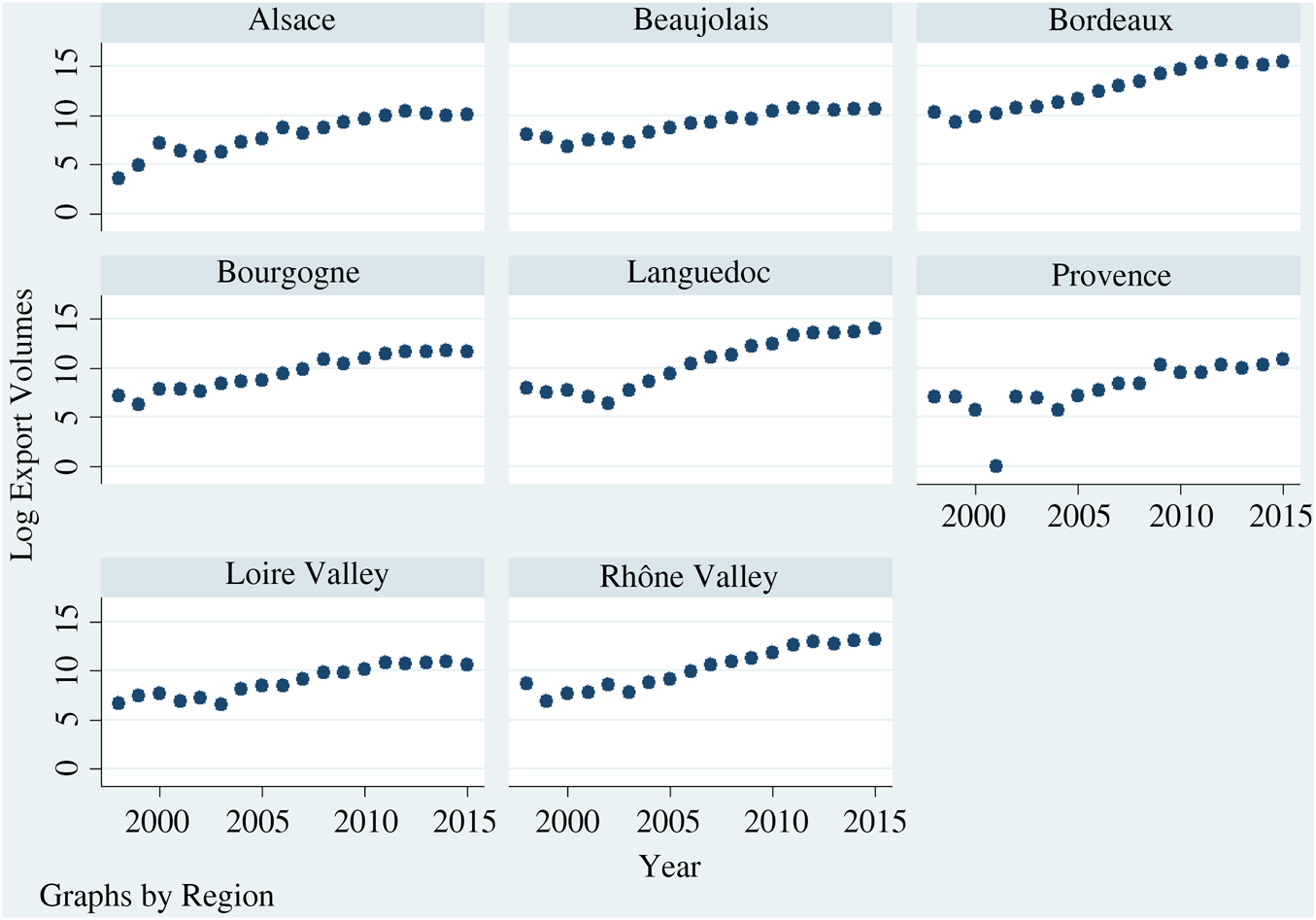
Figure 1 Trends in (Log) Export Volumes to China by French Regions
C. Demand Model
I assume that China's utility function for foreign wine is separable independent across the different wine-producing countries. This is a plausible assumption because the wines made in different countries are as different as the wines made in the different French regions. Moreover, French wines have particular reputations, import channels, etc., which make the zero cross-price elasticity assumption credible.Footnote 5 Following this logic, I focus on the second stage of a two-stage budgeting problem (Gorman, Reference Gorman1959) whereby the demand across different types of French wine is made conditional on the total Chinese expenditure of French wine.
I rely on a standard demand system, with several options for its specification. The first one is to adapt standard forms (like Rotterdam, AIDS, and QUAIDS models) to the present setting. Price aggregation is not necessary; since the overall Argentinian or Spanish price indices are common to all French regions, they will only enter as time shifters. Since I consider deal trade flows, I opt for a simple specification resembling that of a gravity model (see, e.g., Anderson and Van Wincoop, Reference Anderson and Van Wincoop2003, Reference Anderson and Van Wincoop2004; Head and Mayer, Reference Head, Mayer, Gopinath, Helpman and Rogoff2014) but simplified to the extreme: one importer and one exporter. I then disaggregate this using appellation-level or regional-level exports, in the spirit of trade models using firm export data (e.g., Crozet, Head, and Mayer (Reference Crozet, Head and Mayer2012), in the case of Champagne firms).
The most frequent approach used in the empirical literature is the log-linearized form of the gravity equation. This model in its most disaggregated form—that is, at the appellation level i—is written as

where X irt represents the volume of French bottled wine exports to China for appellation i from region r at time t, Y t is the GDP of China at time t, RER jt is the bilateral RER between the two countries, UV irt is the unit value taken as a proxy for the unitary price of the wine of appellation i, and X irt is a set of additional controls that will be introduced step by step in a sensitivity analysis (information about tariffs, Chinese wine production, or specific events).Footnote 6
I include a linear time trend λt to capture the unobserved trade determinants that are common to all French regions. In such a simple model, this term absorbs all linear variations, so that the effects of variables like GDP, exchange rate, or tariffs will be identified in the model inasmuch as they show sufficient nonlinearity or discontinuity over the years under study.Footnote 7 Note that common but unrelated time trends between exports and key time-varying explanatory variables would cause a spurious regression problem; including a time trend then implicitly detrends these series and will guarantee their stationarity, as shown later. In the sensitivity analysis, I will also include appellation fixed effects θ i to control for time-invariant differences across appellation (like long-term reputation or appreciation by Chinese customers) or, alternatively, region fixed effects θ r.Footnote 8
Regions are also interacted with key variables—GDP, RER, and unit values—to provide heterogeneous effects, as characterized in the model

This model should remain parsimonious by ignoring other time-varying variables; estimations will be conducted while making only one of the coefficients heterogeneous at a time—essentially γ 1r first, for income effects, then γ 3r for price effects. I did not find any heterogeneous effects of the RER and these results will not be presented.
D. Stationarity and Cointegration Tests
Before moving to the main results, I report a few tests to examine the integration order of the main variables in the model: log volume, log Chinese GDP, log unit values (taking the annual average over all French wines for simplicity), and log RER. For each of them, I run the Augmented Dickey–Fuller (ADF) test with two lags. The null hypothesis that the variable contains unit roots is rejected for log volumes (p-value of .07) and unit values (p-values of .05), but not for the other two variables. For log GDP and log RER, the time series is not stationary. Standard solutions are first differences (in case of stochastic trends) and detrending (in case of deterministic trends). Both approaches show that log GDP and log RER are I(1), that is, become stationary at standard significance levels.Footnote 9 The fact that both approaches give similar results, and could alternatively be used, is reassuring. Indeed, first differencing is not a favorite choice in this context for three reasons. First, region fixed effects vanish in first differences, which is an issue since regional effects are of specific interest for this article. Second, results in levels are not equivalent to results in first differences—the former implies the latter, but not vice versa. This is the motivation behind cointegration checks of long-term relationships between time series—standard cointegration tests actually point to the existence of such a relationship between the dependent variable (export volumes) and its key determinants (e.g., GDP).Footnote 10 Third, it is much easier to interpret results in levels once a time trend is included in the model, as specified in Equations (1) and (2), which implicitly account for the detrending of all relevant time series contained in the model.
IV. Results
I proceed with the estimations of (log) export values, at year x appellation levels, on a different set of regressors in a stepwise approach. Results are reported in Table 1. As explained earlier, I essentially focus on the sample, excluding zero trade flows (intensive margin) in Models 1–5. I also include zeros in Model 6 by using a simple transformation of the dependent variable, namely log (X + 1), to obtain marginal effects comparable to those in the previous log-linearized models.Footnote 11 All models control for time trends.
Table 1 Determinants of French Wine Exports to China (Log Volume)

OLS estimations on export values. Reference Region: Provence. Standard errors in parentheses. *** p < 0.01, ** p < 0.05, * p < 0.1
A. Main Trade Determinants: Income Effects, Price Effects, and Exchange Rates
In the first column of Table 1, I retain only the basic variables, namely the logarithms of the GDP, the RER, and the unit value, respectively, without any control for appellation or region. The coefficient on log(GDP) suggests a large, highly significant income elasticity of Chinese demand for French wine. The demand elasticity with respect to the exchange rate is small and not significant. The price elasticity of demand, captured by the log unit value, is negative, as expected, and statistically significant.
The next columns introduce additional controls. Throughout, the main variables—log GDP and log unit value—show great stability with significant effects and relatively constant magnitudes. The coefficient on the yuan/euro real exchange rate is negative in most specifications, as expected, but remains, for the most part, insignificant. Note that the absence of a strong effect is not necessarily related to the control for a linear time trend in the model. First, it could be identified in spite of the latter, given the nonlinear trend of the exchange rate.Footnote 12 Second, alternative unreported estimations without a linear time trend still show insignificant effects of the RER; yet, times series suffer from non-stationarity in this case, including the log RER. Note that Song and Liu (Reference Song and Liu2017) also find insignificant exchange rate elasticities in the bottled wine market.
The results for log(GDP) point to an income elasticity of demand larger than 1 suggesting that wine is a luxury good in China. It varies between 3.7 and 4.7 across specifications, which is within the range of the results of Song and Liu (Reference Song and Liu2017), who find an elasticity as high as 6 for France, and Muhammad et al. (Reference Muhammad, Leister, McPhail and Chen2014), who find an elasticity between 1 and 2. In the latter study, French wine is characterized by one of the highest income elasticities among all wine trading partners of China over the period studied. Income elasticities larger than 2, as in this present study or in Song and Liu, may appear unusually large. Nonetheless, there exists evidence of large elasticities in previous studies. For instance, Labys (Reference Labys1976) reports income elasticities above 2 for the United States, at a time when annual wine consumption was much lower than today (around 3 liters per capita) and, hence, more similar to current Chinese levels (in the order of just above a liter, cf. Figure A2).
Across the different specifications of Table 1, the unit-value elasticity is in a range between –.74 and –.60, which is close to the elasticity of –.81 reported by Muhammad et al. (Reference Muhammad, Leister, McPhail and Chen2014) using international variation in wine imports to China. Song and Liu (Reference Song and Liu2017) do not find significant price effects. The elasticity they report for France is similar, –.56, but it only concerns bulk wine while I focus on bottled wine. Both studies show that French wine is close to the lower bound of price elasticities compared to other countries, showing that Chinese consumers are not very sensitive to prices regarding French wine. I will refine this analysis by showing that there is, in fact, a lot of variation across French regions in this respect.Footnote 13
B. Additional Results
(1) Additional Covariates
In Column (2) of Table 1, I include tariffs and the production level of Chinese wine. Tariffs have a negative sign, as expected, but are not significant. The coefficient on Chinese production may have a positive sign if it corresponds to a boom in Chinese interest for wine during the period and a demand for variety, or a negative one if it translates substitutability and competition between French and Chinese wines. The overall effect is positive but usually insignificant (except in one specification). As noted previously, the identification of a clear pattern for both tariffs and Chinese wine production is difficult in a model where most of the variation is time-based.
In Column (3), I account for potential time discontinuities corresponding to specific events, specifically the launch of an anti-corruption policy in China (2012) and the Great Recession (2008–2009). The austerity and anti-corruption policy have heavily impacted official banqueting and expensive gift-giving, subsequently affecting the consumption of expensive wines and other luxuries. I expect this to have only a minor impact on lower-quality wines, which are by far the most voluminous. Nonetheless, this policy explains, in part, the difficulties experienced by other exporting countries like Australia, as documented by Anderson (Reference Anderson2015). The results show no specific effect of the anti-corruption year (I use a dummy switching to 1 in 2012 and subsequent years) once all the other controls are included—which is somewhat different from what the descriptive statistics convey (an overall decline in exports). A similar conclusion emerges from the crisis effect; it carries a negative sign but is rarely significant (I use a dummy switching to 1 for 2008–2009).
In Column (4), I add appellation fixed effects θ i and in Column (5), French region fixed effects θ r. In both cases, the main conclusions regarding income and price effects are unchanged. The R-squared increases .87 with the inclusion of appellation fixed effects, as the panel dimension is now fully accounted for. Estimates of the main covariates are more precisely estimated, pointing this time to a significantly negative effect of the exchange rate, a significantly negative effect of the Great Recession, and a significantly negative effect of tariffs. Controlling only for regional fixed effects, in Model 5, does not seem to be enough for these additional results to hold. However, this specification allows an examination of conditional regional effects. Conditional on all the variables of the model and, in particular, wine unit values for each appellation at each point in time, the long-term effect of certain regions comes out significantly. Relative to the omitted category (Provence region), a market advantage for Bordeaux is seen. There is also a negative effect for two regions, the Loire Valley and Alsace, which primarily produce white wine. This may be due to the long-term preference for red wines among Chinese customers.
(2) Adding the Extensive Margin
In Column (6), I estimate the model using both zero and nonzero observations, that is, additionally including appellations for which there was no export to China in given years (31% of the initial sample). In this model, there is no information about prices. For other variables, conclusions are obtained that are very similar to the pure intensive margin case, at least regarding income elasticity and regional effects. The role of additional variables like tariffs, Chinese production, and time events is somewhat reduced in this model.Footnote 14
(3) Heterogeneity by Color
I replicate these estimations separately for red/rosé wines and white wines; results can be found in Tables A2 and A3 in the Appendix, respectively. Contrasted results may again denote the fact that China has very marked preferences. Around 90% of the wine consumed in China is red, a preference rooted in Chinese culture where red is associated with celebrations, happiness, luck, and prosperity (e.g., Capitello et al., Reference Capitello, Charters, Menival and Yuan2017). There also appears to be a gender component to this long-term trend; the increasing demand for white wine is primarily due to the increased wine consumption of Chinese women (Muhammad et al., Reference Muhammad, Leister, McPhail and Chen2014).
The estimates in Table A2 are very similar to the baseline for red/rosé, both in terms of the significance and the magnitude of the coefficients. Given the overwhelming share of red wines in Chinese wine consumption, this is of little surprise. The relative lack of success of Loire Valley and Alsace is apparent here. Since these regions are mainly producers of white wines, their presence in China is not strong. In Table A3, there appear to be slightly lower income effects, which denote a lower preference for white wines in China. The relative disadvantage for Loire Valley and Alsace tends to disappear when considering white wines, especially when I focus on the intensive margin only (Model 5). The reputation of Bordeaux, however, may be so strong in China that it guarantees an export advantage, even regarding white wines.
C. Regional Heterogeneity
I now focus on the main determinants of demand—income and price—and their heterogeneous effects across French regions, as specified in Equation (2). I use a model similar to Model 5, that is, including all controls and adding region fixed effects, while interacting dummies for all wine regions with log(GDP) first and then with the logarithm of unit values. The results are presented in Column (1) of Table 2.
Table 2 Regional Heterogeneity in the Determinants of French Wine Exports

OLS estimations on export values (zero excluded). Standard errors in parentheses. *** p < 0.01, ** p < 0.05, * p < 0.1. All estimations include controls as in Table 1 (log real exchange rate, log Chinese production, log tariffs, time variables) and region FE. Columns (1) and (2) from two separate regressions with regions x log GDP and regions x log Unit Value respectively. Columns (1') and (2') from a single regression with all interaction terms.
(1) Income Effects
Income effects vary in a broad interval from 1.2 for the Beaujolais region to 2.8 for the Bordeaux region. This heterogeneity is not dissimilar to country variations in international studies, which show that wines from the “old world,” and from France, in particular, are favored by Chinese consumers (Muhammad et al., Reference Muhammad, Leister, McPhail and Chen2014). Here, within-country analysis suggests that among French wines, Bordeaux is very recognizable to Chinese consumers. However, another region appears: Languedoc. This could reflect an increasing demand for more moderately priced wine and/or new trends of Chinese investments in regions other than Bordeaux.Footnote 15 Rhône, Bourgogne, and Provence come close in terms of income effect, mixing top and intermediary appellations. Column (1′) reports estimates from a model combining both heterogeneous income effects and heterogeneous price effects. For the former, it suggests that Bordeaux and Languedoc wines are leading the way. This is true, in general, and for red wines and white wines alike, as shown in Table A4 in the Appendix, where I report separate estimations by color.
(2) Price Effects
In Table 2, Column (2) shows that price effects range from –.23 (Bordeaux) to –1.7 (Alsace), and are significant for most regions. Column (2′) reports similar results in the model, including both income and price effects by region. With the latter model, price effects range from –.26 (Bordeaux) to –1.6 (Languedoc). For comparison, note that the values of regional within-country variations are to the cross-country variations reported by Muhammad et al. (Reference Muhammad, Leister, McPhail and Chen2014), where price elasticities range from –.67 (Australia) to −2.0 (the United States). Note that Bordeaux and Languedoc have similar income elasticities but exhibit different price elasticities. The demand for Bordeaux wine is relatively inelastic to price variations compared to all other French wines, which is consistent with its success among Chinese consumers. In contrast, the high price elasticity of the demand for Languedoc wine points at its position in a lower-price segment associated with middle-class Chinese customers, for whom price matters.
These differences will become less significant, however, when focusing only on red wines (see Table A4). Much of the heterogeneity seems to be driven by white wines. Because white wine is not traditionally the first choice in the Chinese consumption market, demand tends to be more responsive to price conditions. This is especially true for white wines of Languedoc or Alsace, but also for the red wines produced in regions usually associated with white wine (Loire Valley and Alsace).
The last two columns of Table 2 report estimates of a regression of the log values rather than log volumes.Footnote 16 Results are the same mechanically in terms of income effect, so the focus is on price effects. It appears that the large price responsiveness of wines from regions like Alsace or Languedoc carries over to the price elasticity of expenditure in value; an increase in the price of these wines tend to decrease the export value. Other regions show more neutral effects as if their prices were set more optimally to maximize benefits. There are two exceptions: Bordeaux and Bourgogne. The most famous regions show little price responsiveness for volumes, which leads to positive price elasticities for export values. A price increase applied to large exported volumes more than compensates for the drop in volumes due to responses to the price variation.
D. Out-of-Sample Prediction and Forecast
I now check the quality of out-of-sample predictions. The demand model is estimated using observations for 1998–2009. The model contains only log(GDP) (interacted with regions), log unit value (interacted with regions), exchange rates, and region fixed effects. Then, I predict demand volumes for all years. Figure 2 shows both actual and predicted demand at all year and the 95% confidence bounds of the prediction. The fit is good for both out-of-sample years (2010–2015) and in-sample years (1998–2009). While the confidence interval of the predictions for the years 2010–2015 is arguably large, it always contains the actual demand level.
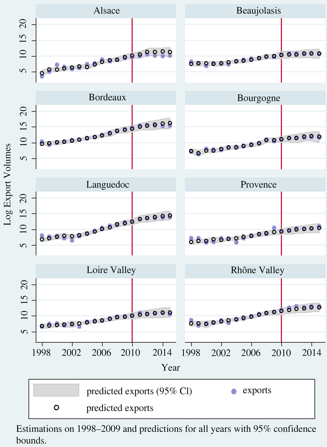
Figure 2 Out-of-Sample Prediction Wine Exports
This model lends confidence to the predicted association between Chinese demand for French wine and the key factors income and price. Based on this model, I now run demand predictions until 2022, holding prices and exchange rates constant. Note, this out-of-sample regression is not a full-fledged forecast, but only a sensitivity analysis showing plausible income-driven demand variations. Exogenous GDP prospects are obtained from the World Bank,Footnote 17 suggesting a slight decline in growth rates, from 6.9% in 2015 to just above 6% in 2022.
The results in Figure 3 show a sustained progression in Chinese demand for all types of wine, with an average annual growth rate of 15% for 2018–2022. The forecasting exercise of Song and Liu (Reference Song and Liu2017) yields an average annual growth rate of 20.5% for the same period (compared to 10% per year over 2012–2016).Footnote 18 Arguably, this figure is not comparable to mine as it derives from a model estimated on cross-country variation, using more demand factors and assumptions regarding their future trends. It does point to a similar conclusion; other things being equal, exports of French bottled wine is likely to continue to grow at a fast pace due to Chinese income growth. In fact, the income effect alone leads to an annual growth rate over 2018–2022 of around 17.7% for Languedoc, 15.9% for Bordeaux, 13.8% for Bourgogne, and 11% for the Loire Valley and Beaujolais.

Figure 3 Extrapolation until 2022
V. Conclusion
The role of China on the global wine market is of growing importance, in particular, because of the large demand driven by middle- and upper-income customers. It is vital for major exporters such as France to understand how the key economic determinants of demand come into play and how their effects may vary across the main exporting regions of the country. Using detailed data on French wine exports to China, I estimate a demand model for the period 1998–2015 and focus on the effects of standard determinants (income and price) overall and by French regions. I find a good deal of within-country heterogeneity, not unlike the amount found in cross-country studies. Bordeaux wines seem to remain China's favorite over the period, with the largest income elasticity. Other regions like Languedoc, however, are gaining recognition with an equally high marginal willingness to pay. The price elasticity is particularly low for famous wines (Bordeaux and Bourgogne); it is the largest for wines targeted at middle-class customers and for wines from regions traditionally known for white wines. Estimations on a sub-period provide a good out-of-sample fit.
Future research could complete these results as follows. First, the comparison with cross-country differences is alluded to in this article but could be further expanded with more data. In particular, it would be interesting to pool expert data from different regions of the world and decompose country and regional effects. Second, one could go further in terms of explanatory variables by using determinants that vary across regions (in my empirical application, only prices vary by region). Third, I have focused on standard income and price effects. One could further explore both “push” and “pull” factors that explain why certain regions export more than others. This could include export policies conducted by specific regions in France (aiming to promote local wines), joint actions by cooperatives in some French regions (which may include production cost sharing, e.g., mutualizing equipment, joint marketing campaigns, etc.), or specific cultural links. It would also be interesting to study variation within China (by income group, education level, urban status, region, etc.), but the data requirements are high.
It is difficult to outline the policy implications of these results—I have emphasized the limits of the predictive work. However, the income elasticities can tentatively be used to quantify—per region—the future of French exports in relation to the current slowdown in Chinese growth. Projections for 2018–2022 suggest that, on the basis of reasonable income growth prospects, the demand for French wine will continue to rise, but not as fast as in the past and at different rates across regions (i.e., with an annual growth rate ranging from 10% to 17%). Price elasticities could also be used for the economic councils of different regions of France to advise local producers on price policies and how they could adjust prices relatively to other regions. I could not detect significant cross-price elasticities across regions, but more comprehensive datasets, combining regional and international export information, could attempt to identify which world wine (e.g., Argentinian Malbec) may be a substitute for French local wines (e.g., French Malbec from Cahors) and possible implications for the respective price policies.
Appendix
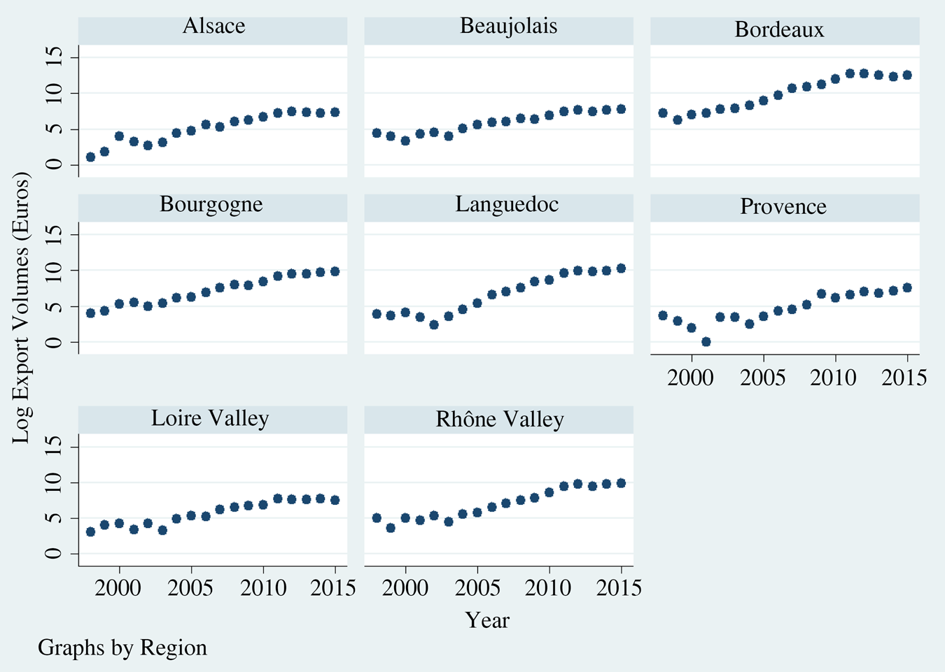
Figure A1 Trends in (Log) Export Values to China by French Regions
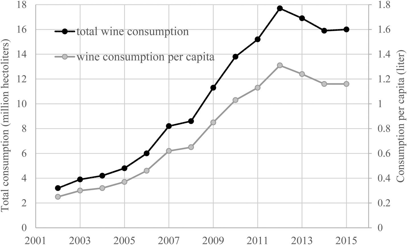
Figure A2 Total and Per Capita Wine Consumption in China
Table A1 (Log) Export Values and Volumes to China by French Regions

Table A2 Determinants of French Wine Exports to China (Log Volume), Red and Rosé
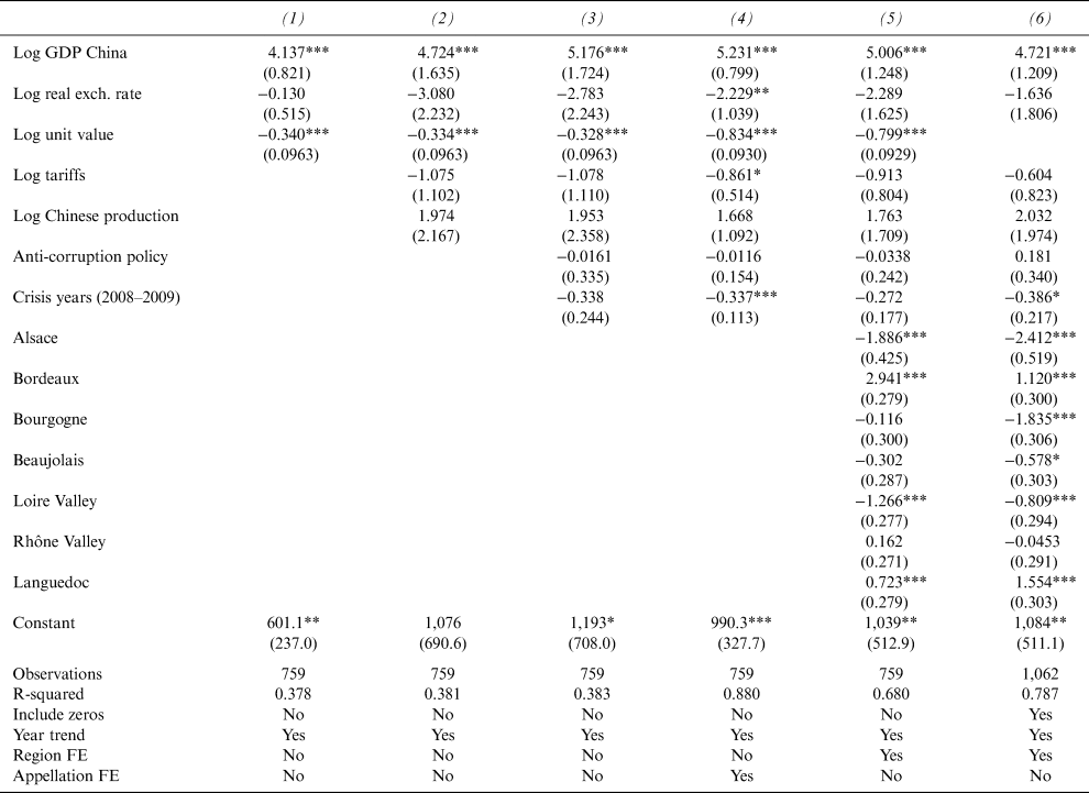
Table A3 Determinants of French Wine Exports to China (Log Volume), White

Table A4 Regional Heterogeneity in the Determinants of French Wine Exports, by Color


