


I. Introduction
Many researchers have studied the price dynamics of fine wines and other collectibles. This paper seeks to expand this body of knowledge in two ways. First, by leveraging age-period-cohort (APC) models and discussing their similarities to and differences from the prevailing techniques, a large body of literature on technical details of vintage modeling can be brought to fine wines. Secondly, with access to a new and unique database, we can not only test previous results but also ask new questions.
APC models can be applied to any vintage-based data. This process occurs in many fields, but most notably in actuarial studies, medical studies, consumer loans, and product forecasting, to name a few. APC models have been one of the dominant statistical techniques in the social sciences for understanding long-term behavior (Holford, Reference Holford1983). In the last decade, this technique has reached prominence for the US Federal Reserve's stress-testing program for consumer loans (Breeden, Reference Breeden2010; Breeden and Canals-Cerda, Reference Breeden and Canals-Cerda2016). Most recently, the Federal Accounting Standards Board has identified “vintage models” as a preferred method for predicting loan losses (Financial Accounting Standards Board, 2016). Thus, APC models are a generic technique for taking performance data from separate cohorts and decomposing the data into independent functions of vintage quality, life cycle versus age, and environment versus time. One strength of APC models comes from their early recognition of the model specification error that arises from analyzing age, vintage, and time effects simultaneously. Section II discusses this factor in detail along with its implications for analyzing wine prices.
Because we use the APC algorithm to model constituent drivers of price sensitivity, it falls within the class of hedonic regression (Rosen, Reference Rosen1974). The APC modeling technique is also similar to repeat sales regression (Bailey, Muth, and Nourse, Reference Bailey, Muth and Nourse1963), which assumes that the log appreciation rate equals the log appreciation rate of an environment plus an error term. Log differences of repeat sales are regressed on time dummies. Although similar in concept to looking at recurring sales, the APC model in this case is applied directly to price values rather than to price differences. We make this choice when setting up the APC algorithm because of the nonuniformity of the time data.
Not all hedonic regressions of wine prices consider all three dimensions of age, vintage, and calendar date, nor do they all include the detailed treatment of the implicit specification error in vintage data. Therefore, we hope our employment of APC models provides a useful example of how to model age, vintage, and time effects while managing the linear specification error.
Leveraging the database available here, we select three segments for analysis: Château Lafite Rothschild, Bordeaux excluding Lafite, and Burgundy. Château Lafite Rothschild is moved to a separate segment, because the volume of auction data for that wine is sufficient for an independent analysis. Further, anecdotal evidence of specific investor interest in Lafite over the last decade warrants an investigation thereof. The results of this analysis are compared where possible to previous studies for confirmation or divergences. See Storchmann (Reference Storchmann2012) for a detailed survey of the literature.
The life cycles from this analysis are compared across segments and to examples in the literature to illustrate the intrinsic appreciation potential. Note that the analysis is not segmented by the quality of the vintage, as is done in some studies (e.g., Dimson, Rousseau, and Spaenjers, Reference Dimson, Rousseau and Spaenjers2015). Given that the auction volume in the database is dominated by trades of desirable vintages, the results here are essentially those of the best vintages. Future analysis could consider explicit segmentation by quality of vintage.
The current analysis is most similar to that of Dimson et al. (Reference Dimson, Rousseau and Spaenjers2015), who examine the impact of aging on wine prices and, by using a value-weighted arithmetic repeat sales regression over 1900–2012, the long-term return for high-end wines. They create annual price histories for vintages of Haut-Brion, Lafite-Rothschild, Latour, Margaux, and Mouton-Rothschild and analyze those to discover the price-appreciation life cycle with wine age, environmental impacts with calendar date, and included production and quality as explanatory variables to explain vintage variation. Where their research benefits from the long-time history in their data, the current research benefits from the extraordinary breadth of the available data. This information allows us to confirm the extent to which an analysis of five wines over a long history agrees with that of thousands of wines over a couple of decades.
For the APC analysis, the impact of vintage quality on wine prices is handled purely via dummy variables for each vintage. Although it is effective, this approach is not explanatory. It is used initially for the mathematical purpose of supporting the decomposition. A secondary analysis seeks to identify the causes of the variation by vintage.
Because trades of desirable wines here and in many studies dominate the auction data, estimates of the market can be driven by the appreciation of specific, highly desirable vintages as they mature. Therefore, in considering the potential for price appreciation, separating the effects of life cycle and vintage from overall market conditions can be key to understanding potential returns in a specific investment. To this end, the measurement of the environment function from the APC analysis allows for a separate assessment cleaned of price impacts from vintage quality or age of wine.
Prices for fine wines have been analyzed in several papers to determine their suitability as investments (Burton and Jacobsen, Reference Burton and Jacobsen2001; Fogarty, Reference Fogarty2010; Masset and Henderson, Reference Masset and Henderson2010; Sanning, Shaffer, and Sharratt, Reference Sanning, Shaffer and Sharratt2008). For example, Masset and Henderson's (Reference Masset and Henderson2010) study of the evolution of red Bordeaux wine prices from 1996 to 2007 concludes that wines exhibit low correlation to the equity market, making them a useful diversification tool for an equity portfolio, even after taking into account their storage and trading costs. Using a repeat sales regression approach, they study auction prices from the Chicago Wine Company and compare them to Dow Jones Industrial Average (DJIA) market returns. Interestingly, they find strong dependence on vintage and ratings and note that wine prices for a category like Bordeaux move as a group.
Similarly, Sanning et al.'s (2008) study of data from 1996 through 2003 using the Fama–French three-factor model (Fama and French, Reference Fama and French1993) shows that red Bordeaux wines exhibit large excess returns and low correlations to the DJIA and thus may be an attractive investment instrument. Masset and Weisskopf (Reference Masset and Weisskopf2010) use repeat sales regressions to study wine investment returns from 1996 through 2009, with a particular focus on periods of financial crisis. These authors conclude that wine investment, especially in prestigious wines, is a more effective diversification tool during market downturns, offering higher returns and lower risk than equity indices, as measured by the Russell 3000. Masset and Weisskopf use a conditional capital asset pricing model and conclude that wine returns are unrelated to market risk, although they are affected by the state of the US economy.
These analyses can reach different conclusions, based on the methods used and the time periods studied. This variation is demonstrated in a study by Fogarty and Sadler (Reference Fogarty and Sadler2014) of auction-price data from Langton's spanning from 1988 to 2000. The authors compare a range of modeling methodologies to measure the return of wine investment and its diversification benefits. They observe a high degree of variability in the outcome, depending upon the method used and the data range analyzed. Further, they conclude that a repeat sales method would overestimate the returns, while a “pooled model,” which is a modified hedonic model, would work well for wine returns.
Fogarty and Sadler (Reference Fogarty and Sadler2014) also conclude that diversification benefits are small for holding wine as an investment when compared to US and Australian stock and bond indices, and that these benefits are only applicable to portfolios that are close to the “global minimum-variance portfolio” (Kempf and Memmel, Reference Kempf and Memmel2006, p. 243).
We assert that to obtain stable estimates of market impacts on prices, the analysis must separate the effects of life cycle, vintage, and environment. Therefore, after the APC decomposition, the environment function, serving as a market index, is compared to changes in other market indices for correlations or anecdotal structure.
The life-cycle and environment analysis provides industry-level perspectives on wine prices. To obtain more detailed information about the specific lot prices, a secondary analysis is employed. Generally equivalent to discrete time-survival models, panel-data models, or simply generalized linear models, the life cycles and environment from the APC analysis are retained, but the vintage function is replaced with attributes of the lot or the wine vintage.
The coefficients estimated by wine vintage are intrinsically useful at measuring investor interest, but additional analysis is required to identify causes. After the initial estimation of life-cycle, environment, and vintage effects, second-stage models are developed that take life cycle and environment as known impacts and estimate the relative importance of other factors. The key factors considered here are the impacts of wine ratings on prices, the price distribution across different auction houses, and questions of price efficiency by bottle size and lot size.
Section II provides details on the modeling technique employed. Section III describes the database. Sections IV, V, and VI discuss the life-cycle, environment, and vintage outputs of the APC algorithm. Sections VI.A, B, and C discuss the influence of wine ratings, auction houses, bottle size, and lot size.
II. Method of Analysis
We use an APC model to analyze wine-vintage data for the target variables. In the most common applications of APC models, time series of vintage aggregate are modeled. However, the actual estimator does not require continuous time measurements. Because each point is considered independently, inherently nonuniform auction-price data work well.
The basic APC concept is similar to survival and hazard models (Cox and Oakes, Reference Cox and Oakes1984). In all these methods, age is a key determinant of performance (e.g., price in the current context). This is referred to as the life cycle but is also called the hazard function. In this analysis, the “age” is defined as years since the vintage date. The shape of the life cycle is not predetermined, because it can be quite nonlinear in some contexts.
Survival models stop with measuring the hazard function, but other factors also affect performance. Different vintages have different overall price performances, which are quantified as vintage-quality indexes measured relative to the life cycles. Zero for the vintage index means that a vintage is exactly like the life cycle – average price expectation. The vintage function is measured just from the performance data, so the newest vintages lack sufficient performance data for a specific estimate. However, older vintages are well quantified.
One could use a Cox proportional hazards model (Breeden, Bellotti, Leonova, and Yablonski, Reference Breeden, Bellotti, Leonova and Yablonski2015) to estimate the vintage function if that were the only additional driver of performance, but the market environment must also be considered. The environment versus calendar date is again measured as an index whose zero level is set relative to the life cycle. Changes in the environment function indicate how much incremental price in units of log-price occurs on a specific calendar date. Due to environmental influences, periods occur when all vintages attain higher-than-average prices when compared to their life-cycle estimates. This effect is quantified in the environment function.
Mathematically, this approach is expressed as
 $${\rm r}\left( {{\rm a} = {\rm t} - {\rm v},{\rm v},{\rm t}} \right) = {\rm Link}({\rm F}\left( {\rm a} \right) + {\rm G}\left( {\rm v} \right) {\rm H}\left( {\rm t} \right)).$$
The link function depends upon the distribution of the variable being analyzed. In this case, prices show a lognormal distribution, so a log link function is used.
When applied to auction-price data for fine wines, the life-cycle function, F(a), measures the expected average log(price) for a wine in a segment as a function of the age of the wine. Thus, the life cycle captures the expected rate of appreciation in a wine's value across different spans of time.
The vintage function, G(v), measures how much higher or lower a given wine is priced relative to the average life cycle for the segment. This function allows for the estimation of separate price scaling by vintage and the maintenance of a common market index (environment function) and common life-cycle function across all wines in a segment.
The environment function, H(t), measures how much auction prices are above or below the expected life-cycle values on a given calendar date. In this way, the environment function provides a market index that can leverage all wines auctioned, not just those in a select list, and is normalized for the natural appreciation in the value of the wines over time.
APC models as a class are used in many fields, such as economics, biology, sociology, and more. APC models have been in use for more than one hundred years, and their properties and implementations are well known at this point (Holford, Reference Holford, Everitt and Howell2005). The APC algorithm employed here is based upon the Epi implementation in R.
The three functions employed in APC models cannot be estimated in fully nonparametric form, because a model-specification error exists. The age of the vintage is connected to its vintage and observation date as a = t − v. This simple equation means that a linear ambiguity exists, whereby the linear trend can be measured uniquely in only two of the three functions. Many solutions to this problem exist, but all include making an assumption about the allocation of these trends. Yet research has proven that the nonlinear components of the three functions are uniquely estimable (Holford, Reference Holford, Everitt and Howell2005). In the current context, the environment function is assumed to have no net trend. As a consequence, we cannot comment on the long-term market trend, only on the nonlinear aspects of the environment – namely, the degree to which price movements are correlated with other markets.
The specification error is not a feature of the APC model but an attribute of the data. Recent work (Breeden et al., Reference Breeden, Bellotti, Leonova and Yablonski2015) shows that the linear specification error in APC is equivalent to a multicollinearity problem when using a factor-based approach. For example, Dimson et al. (Reference Dimson, Rousseau and Spaenjers2015) recognize the linear specification error in their nonparametric approach. They resolve the problem by replacing the nonparametric vintage function with annual production and taste-quality measures. Although this change makes the equation estimable in a regression context, the answer is no more accurate, because a multicollinearity problem equivalent in magnitude to the linear specification problem still exists between these vintage factors, age of the vintage, and calendar date.
Because the nonlinear structure is uniquely estimable, for very long datasets like that of Dimson et al. (Reference Dimson, Rousseau and Spaenjers2015), most of the structure is captured in the observed variability. However, in comparatively short studies of one or two decades, most of the structure may be captured in the linear trends, so careful consideration should be given to the multicollinearity problem and how it can affect the results. In fact, this consideration is a leading candidate for why studies of wine-market returns yield such different answers.
To estimate the APC functions in a nonparametric form with linear trend control, we follow the Bayesian APC algorithm of Schmid and Held (Reference Schmid and Held2007). Our implementation of this algorithm uses a spline APC estimation as an initial prior and then employs a Monte Carlo estimation procedure to refine the functions. The result looks “noisier” than a spline estimation, but it can better estimate the complex and discontinuous structure that can arise in the functions.
A. Testing Attributes
In addition to the basic decomposition, our research tests specific factors that may influence auction results – namely, the auction house, wine rating, lot size, and bottle size. But to accurately estimate these effects, the data must be normalized for the expected life cycle and market environment to clarify the relationships.
To combine lot attributes with the decomposition, we employ a discrete-time survival model (DTSM) (Tutz and Schmid, Reference Tutz and Schmid2016). DTSM is equivalent to a Cox proportional hazards model, but with the condition that all performance data are in discrete time. Although auction times are theoretically continuous, the life-cycle and environment estimates are not. Therefore, only the month of the auction is considered, and DTSM is appropriate.
Many practitioners use DTSM by simultaneously including in the estimation equation factors of age of the vintage, macroeconomic factors, and lot attributes, thereby combining the preceding APC estimation with factor estimation in a single step. Although single-step solutions are appealing, most datasets exhibit colinearity problems between life-cycle, environment, and explanatory factors. In the present context, the problem is resolved by using the life-cycle and environment functions from the APC algorithm as fixed inputs (coefficients of 1) to the DTSM:
 $$p\left( {a,v,t} \right)\; \sim \;F\left( a \right) + H\left( t \right) + \sum\nolimits_{\,j = 1}^{n_s} {c_j \cdot s_{ij}.} $$
In the above equation, F(a) + H(t) does not have any scaling coefficient in the regression equation. This is called a fixed offset to the model. Consequently, the explanatory factors are capturing the lot-specific variation as a distribution centered around the life-cycle and environment functions.
III. Data
The analysis is conducted on a database provided by auctionforecast.com, covering a fifteen-year time span from the following auction houses: Acker Wines, Bonhams, The Chicago Wine Company, Christie's, Langton's, Sotheby's, Spectrum Wine, Veiling Sylvie's, and Zachys. The provided data adjusted all currencies to US dollars according to the exchange rate on the date of the auction. Prices are in nominal dollars, without adjustment for inflation over time. All prices are hammer prices.
Only auction results for lots containing a single wine vintage are included, and all prices are converted to price per bottle. Although some information is available in the lot descriptions for such factors as “original wooden case” or “damaged label,” these are not included in the modeling database. The number of bottles in the lot is retained as information that can be used in later modeling.
For the subsequent analysis, only wine vintages that have been sold at auction at least sixteen times are included. This threshold minimizes the estimation error relative to individual wine vintages, which roughly scales as
 $1/\sqrt N $
. Excluding less-traded wine vintages is a luxury of having such a large database. Sixteen is chosen experimentally as a threshold simply because it is a number sufficient to minimize the number of unstable coefficient estimates. This threshold retains 2,901 Burgundy wine vintages, 81 Lafite vintages, and 4,222 Bordeaux excluding Lafite wine vintages.
$1/\sqrt N $
. Excluding less-traded wine vintages is a luxury of having such a large database. Sixteen is chosen experimentally as a threshold simply because it is a number sufficient to minimize the number of unstable coefficient estimates. This threshold retains 2,901 Burgundy wine vintages, 81 Lafite vintages, and 4,222 Bordeaux excluding Lafite wine vintages.
Table 1 shows the number of lots by vintage since 1973, chosen as a starting point to capture the majority of the data. Older vintage data are present but do not contribute significantly to our analysis. Table 2 shows the number of lots by calendar year. Auction volume in this database peaks in 2012 but has remained strong. Table 3 illustrates the number of lots by bottle size, showing that 95.1% of all the auctions are for 750mL bottles. Table 4 shows the number of lots by price per bottle. This distribution fits nicely with the log-normal assumption in the later modeling. The peak is in the price range of $80 to $160 per bottle.
Table 1 The Number of Lots by Vintage and Segment since 1973 within the Modeling Database

a Lafite is listed separately from the rest of Bordeaux in this table, because Chateau Lafite Rothschild has sufficient data for an independent analysis.
Note: Older vintages are present in the data in small volumes. This table focuses on the most important contributors to the analysis.
Source: Auctionforecast.com
Table 2 The Number of Lots by Calendar Year in Total for the Segments Modeled within the Database

aOnly lots containing a single wine, vintage, and bottle size were included for analysis.
Source: Auctionforecast.com
Table 3 The Number of Lots by Bottle Size in the Modeling Database

Source: Auctionforecast.com
Table 4 The Number of Lots by Price Tier in the Modeling Database

Source: Auctionforecast.com
IV. Life Cycle
The APC decomposition of wine prices provides several insights into the dynamics of wine prices at auction. The analysis is run separately for Lafite (Château Lafite Rothschild), Bordeaux (excluding Lafite), and Burgundy. Lafite is studied separately because of unique investor interest in these wines and the volume of auction prices available.
As shown in Figure 1, looking first at the price life-cycle function versus the age of the wine vintage, all three segments show the same general behavior. For Lafite and Bordeaux in general, the average auction price actually declines until the fifth or sixth year, at which point the prices stabilize and begin to rise again. For Burgundy, the bottom occurs between the sixth and eighth years of age for a vintage.

Figure 1 Life-cycle Functions for Château Lafite Rothschild, Bordeaux Excluding Lafite, and Burgundy
The most rapid price increases occur in the couple of decades after that minimum before slowing their rate of appreciation throughout the remaining lives of the wines. For Lafite and Bordeaux excluding Lafite, the cumulative price appreciation between five and twenty-five years of age is 81% and 69% respectively, or 3.0% and 2.7% geometric mean return annually. The importance of these estimates is that they are cleaned of changes in market conditions and represent the performance of average Lafite and Bordeaux wines cleaned of differences in specific vintage performance. Although 81% appreciation sounds impressive, 3.0% annual capital appreciation for the wine is less exciting when considering transaction costs, storage costs, inflation, and so forth.
These results agree well with those of previous studies: Dimson et al. (Reference Dimson, Rousseau and Spaenjers2015) report geometric average price appreciation of 2.7% over the first forty years, Di Vittorio and Ginsburgh (Reference Di Vittorio and Ginsburgh1996) report 3.7%, and Ashenfelter (Reference Ashenfelter2008) reports 2.4%. Our quoted results are for the period of most rapid growth, so a longer time interval would show lower average growth rates.
These results on price appreciation are independent of market swings, so they are not sensitive to the time period modeled. This can help explain why some authors find significant appreciation and others do not. Our results appear to agree with those who have stated that wine overall is not an effective investment in comparison to stocks and other investment opportunities if one buys and sells at random times (Burton and Jacobsen, Reference Burton and Jacobsen2001; Haeger and Storchmann, Reference Haeger and Storchmann2006; Jones and Storchmann, Reference Jones and Storchmann2001). However, this agreement does not prove that wine cannot be profitable if the trades are made at the appropriate points in the market or for the right vintages. These results suggest only that buying a broad basket of wines averaged over vintages and market conditions is not likely to be a profitable strategy. Market timing is required for superior returns.
V. Environment
The environment functions measured in the decomposition provide a more refined view of the wine market. Wine-market indices may follow a wine-basket approach or a statistical-modeling approach. For wine baskets, a price index is computed from a collection of desirable wines and vintages. When a vintage passes its period of desirability, it is replaced with a newer wine vintage, and the index is rebalanced. This approach essentially mirrors stock-market indices, such as the DJIA, where individuals are sometimes replaced and the indices are rebalanced to maintain continuity. However, unlike the stock market, wine vintages undergo a maturing process, as described in the previous section, so a wine basket can be biased toward growth as the constituent wines mature.
The current decomposition approach estimates a dummy variable for each time period expressing the change in log-price relative to other periods. Dimson et al. (Reference Dimson, Rousseau and Spaenjers2015) use such an approach to measure the wine market over many decades for the five top Bordeaux wines in their study. Our study does not have the length of history of Dimson et al.’s but can measure the wine market across more than seven thousand wine vintages for the segments considered. This ability provides a broader perspective on movements in the wine market than any index of which we are aware.
As noted in the technical details, any analysis of age, vintage, and time effects (via any modeling technique) cannot distinguish all three trends uniquely. Therefore, if the wine market as a whole were to exhibit a 3% annual appreciation rate, one could not determine whether that were the appreciation rate of the wine vintage versus age or the wine market by calendar date. The effects would not be distinguishable. Therefore, our analysis makes the mathematical assumption that such long-term bias to price growth is included in the price-appreciation life cycle versus age of the vintage. The environment function estimated here has no net trend, but the nonlinearities are very useful for looking at cycles in the wine market and correlating to cycles in other markets.
The environmental functions are shown in Figure 2 for the three segments studied. The function is measured in units of log-price (y-axes) with the zero level corresponding to the long-run average of the dataset. Lafite clearly shows the peak in early 2011, known as the “Lafite Bubble.” From June 2010 to February 2011, prices for Lafite wines, adjusted for life-cycle and vintage effects, jump by roughly 50%. By April 2013, the environment function shows a decline to levels below the June 2010 start of the bubble. The environment function for Bordeaux largely mimics the Lafite function, although with an even more pronounced peak between April 2010 and July 2011, suggesting that the “Lafite Bubble” label does not fully capture the breadth of the market event.

Figure 2 Environment Functions for Château Lafite Rothschild, Bordeaux Excluding Lafite, and Burgundy
Visually, we see periods when the Lafite and Bordeaux excluding Lafite environment functions move coherently with the Hong Kong and Shanghai stock-market indices from January 2006 through May 2014 (see Figures 3–8), offering some evidence that Chinese wealth may have been driving the fine-wines market. Burgundy appears to be uncorrelated to the stock-market indices but retains some correlation to Bordeaux wines. But since the end of 2012, all environment functions have exhibited steady, significant declines, regardless of stock-market movements. Fine wines appear to have been in a bear market through mid-2015.

Figure 3 Comparisons of the Lafite Environment Function and Shanghai Stock Market Index, in Levels and Quarterly Log-Returns

Figure 4 Comparisons of the Lafite Environment Function and Hong Kong Stock-Market Index, in Levels and Quarterly Log-Returns

Figure 5 Comparisons of the Bordeaux Environment Function and Shanghai Stock-Market Index, in Levels and Quarterly Log-Returns

Figure 6 Comparisons of the Bordeaux Environment Function and Hong Kong Stock-Market Index, in Levels and Quarterly Log-Returns

Figure 7 Comparisons of the Burgundy Environment Function and Shanghai Stock-Market Index, in Levels and Quarterly Log-Returns

Figure 8 Comparisons of the Burgundy Environment Function and Hong Kong Stock-Market Index, in Levels and Quarterly Log-Returns
Table 5 summarizes the correlations between wine-market returns and stock-market returns. It shows that Lafite and Bordeaux excluding Lafite correlations to Chinese stock-market indices are comparable to the correlations between wine categories. We test correlations to US and European stock-market indices and find no useful structure, in line with what other authors observe.
Table 5 Correlations of Quarterly Log-Returns

aBordeaux excludes Chateau Lafite Rothschild in this analysis, so that interest in Lafite could be studied separately.
Note: The quantities in parentheses show the minimum and maximum values to 95% confidence.
Source: Authors’ model results.
Conventional wisdom is that the “Lafite Bubble” was caused by a sudden increase in interest from Chinese investors. Interestingly, the Lafite environment function moves coherently with the Shanghai stock-market index throughout this same time frame. This finding is different from that of previous studies. Most of those studies consider correlations only to US stock-market indices, which also appear to be uncorrelated here. None appears to have considered the impacts of the Chinese market. This finding agrees with earlier literature, such as Masset and Weisskopf's (Reference Masset and Weisskopf2010) study of the period of 1996–2009, which concludes that wine-investment returns have little correlation to the stock market when considering the US market.
As noted by other authors, the correlation results can depend strongly upon the time period studied. For example, Sanning et al. (Reference Sanning, Shaffer and Sharratt2008) show that wines as an investment exhibit large excess return (more than 0.60% to 0.75% per month and 7.5% to 9.5% per year of excess return) and have little exposure to market risk, but their study does not include the market correction after 2011.
Our analysis does not speak to whether this correlation would be stable going forward, nor do we expect to observe these correlations in long histories, such as Dimson et al.’s (2015), because the Chinese were not wine buyers then. The current results seem to support anecdotal reports from wine merchants that the Chinese exhibited a significant influence on the Bordeaux market during this period.
VI. Vintages
In subsequent analysis, the vintage function above is replaced with lot-specific attributes for detailed analysis. Initially, however, the vintage estimates are interesting as a nonparametric measure of the most popular vintages, normalized for environment and life-cycle affects.
Figure 9 shows some broad structure, such as the strong trend with vintage year for higher Lafite prices. When looking at the relative peaks, the following vintages exhibit exceptional price appreciation: 1982, 1986, 2000, 2005, and 2006 for Lafite; 1982, 1990, 1992, 2005, and 2008 for Bordeaux excluding Lafite; and 1985, 1991, and 2003 for Burgundy. Notable in this analysis is that the most valuable Château Lafite Rothschild wines do not always coincide with the most valuable Bordeaux wines generally. In addition, the best Burgundy vintages show no overlap with the best Bordeaux or Lafite vintages.

Figure 9 Vintage Functions for Château Lafite Rothschild, Bordeaux Excluding Lafite, and Burgundy
Among the most significant literature in this area is written by Ashenfelter (Reference Ashenfelter2008), who reports using the “Bordeaux equation” that a 1 degree Celsius increase in temperature during growing season results in a 61.6% price increase (Bailey et al., Reference Bailey, Muth and Nourse1963). Ashenfelter's work considers the age of the wine at the time of sale as a linear function of the château and the weather. The analysis highlights the 1989, 1990, 2000, and 2003 vintages as exceptional based upon the weather, and some overlap can be seen with the results here. He also notes that although weather conditions predicted 1982 to be good, the auction prices far exceeded those predicted from the fundamentals.
We cannot know the extent to which not normalizing for market conditions accounts for the difference in vintage assessment, but we do see some general agreement on which vintages are most valuable. Storchmann (Reference Storchmann2012) notes that most of the studies use linear temperature specifications, which work better in cooler climates than in warmer ones. In warmer climates, Storchmann believes that nonlinear specifications are more suitable.
A. Lot Size and Bottle Size
Section VI utilizes the generalized linear-models approach to replace the vintage function with estimations of specific lot attributes. The APC-estimated life cycle and environment are included as fixed effects:
 $$\eqalign{\,p\left( {a,v,t} \right)\; & \sim\; F\left( a \right) + H\left( t \right) + c \cdot bottle\_size \cr &\quad + d\cdot lot\_size + e \cdot rating + f\,\cdot auction\_house} $$
In the above equation, bottle_size, lot_size, rating, and auction_house are all categorical variables, so the estimated coefficients c, d, e, and f are vectors of coefficients for the discrete levels of those attributes.
Rather than post a single long table of coefficients, these sections provide specific discussions of each explanatory variable. First is the dependence on lot size. The estimation is performed on log price per bottle, but if the market is inefficient, the number of bottles in a lot (lot_size) may contribute to the estimation. Table 6 shows the coefficients by lot size. Although a couple of values show significance, the result overall appears random. We conclude that the auction data are efficient with respect to the number of bottles in a lot.
Table 6 The Coefficients by Lot Size (Number of Bottles per Lot) Showing the Adjustment to Log Price

Note: Error and significance estimates are included.
Source: Authors’ model results.
This result actually may disagree with the previous literature. Ashenfelter (Reference Ashenfelter1989) relates the story of the first English auction he experienced, where he witnessed the declining price for identical lots based on the order in which they were sold. Ashenfelter reveals that auction houses often attempt to disguise this phenomenon, placing smaller lots of the same wines before the larger lots, and, when a series of identical lots is offered, giving the first lot winner the option to purchase the subsequent lots at the same price. Ashenfelter points out that the price-decline anomaly in wine auctions is present in auction houses in London and in the United States. Ginsburgh (Reference Ginsburgh1998) further investigates the declining-prices effect using data gathered from four sales at Christie's London between December 1995 and February 1996. Ginsburgh finds that the declining prices are likely to be caused by the fact that most bids are entered by absentees.
The current data do not indicate the order of the lots, so no conclusion can be drawn about price declines across them. The previous studies indicate that a correlation exists between lot size and lot sequence and thus affects price. Although that may be true, the signal appears to be lost in the larger dataset.
Although the auction prices appear to be efficient in lot size, bottle size shows a significant effect in our study. Table 7 shows the estimated values based upon bottle size. All estimates are relative to a standard 750mL bottle. The “ideal” values show the coefficients that should have been obtained if market prices were efficient. The result shows that all bottles sizes other than the standard 750mL bring lower prices per volume, sometimes significantly so. For those purchasing to consume, nonstandard sizes can provide bargains.
Table 7 The Coefficients by Bottle Size Showing the Adjustment to Log Price

Note: Error and significance estimates are included. The ideal values show what should be obtained if the market is efficient with respective to the volume of wine in the bottle.
Source: Authors’ model results.
B. Wine Ratings
The database includes enough Wine Advocate and Wine Spectator ratings to support a useful statistical analysis. In general, wine ratings are the subject of much debate. Storchmann (Reference Storchmann2012) includes literature showing that so-called experts can provide little or misleading information. Hodgson's study (Reference Hodgson2008) shows that experts award medals to wines at random, and Reuter (Reference Reuter2009) shows that conflicts of interest may play a role in biased outcomes. Cardebat and Paroissien (Reference Cardebat and Paroissien2015) develop a method of translating expert opinions to scales comparable to the Parker scale.
Further, Cardebat and Livat (Reference Cardebat and Livat2016) examine whether the lack of consensus in expert ratings is due to the experts’ personal preferences. They find that some experts tend to prefer wines from a certain region, which is often related to the geographical region of the experts themselves. The authors argue that this bias does not mean inefficiencies in the region but that consumers benefit from finding the “right experts” (p. 43).
Our research does not attempt to explore the reliability or usefulness of wine ratings for taste; instead, we focus on the extent to which wine prices may correlate to wine ratings. Wine ratings are included as categorical variables in the analysis to test for a relationship to log prices. Equation 3 is estimated separately with Wine Spectator and Wine Advocate ratings as the input variable to assess each independently.
Wine Spectator and Wine Advocate ratings have similar monotonic behavior relative to log-price and even a similar scaling, with the significant exception of the highest-rated wines. For Lafite and Bordeaux excluding Lafite, 99-rated wines are dramatically more valuable than 98-rated wines at auction, but 100-rated wines exhibit auction values at the level of wines rated at 98 or less. Although the confidence intervals on the estimates are large, the drop for 100-rated wines is significant. For Burgundy, 100- and 99-rated wines are lower than those rated at 98.
All the measured dynamics in this analysis are relative to auction price rather than opinions on the taste of the wine, but the tests do show a strong relationship between price and rating for Lafite, Bordeaux, and Burgundy in Figures 10, 11, and 12, respectively. Wine Advocate ratings show a fairly smooth, monotonic relationship to differences in log-price. For Bordeaux, the difference between an 85-rated wine and a 100-rated wine is roughly a factor of 100 in price throughout the life of the vintage.
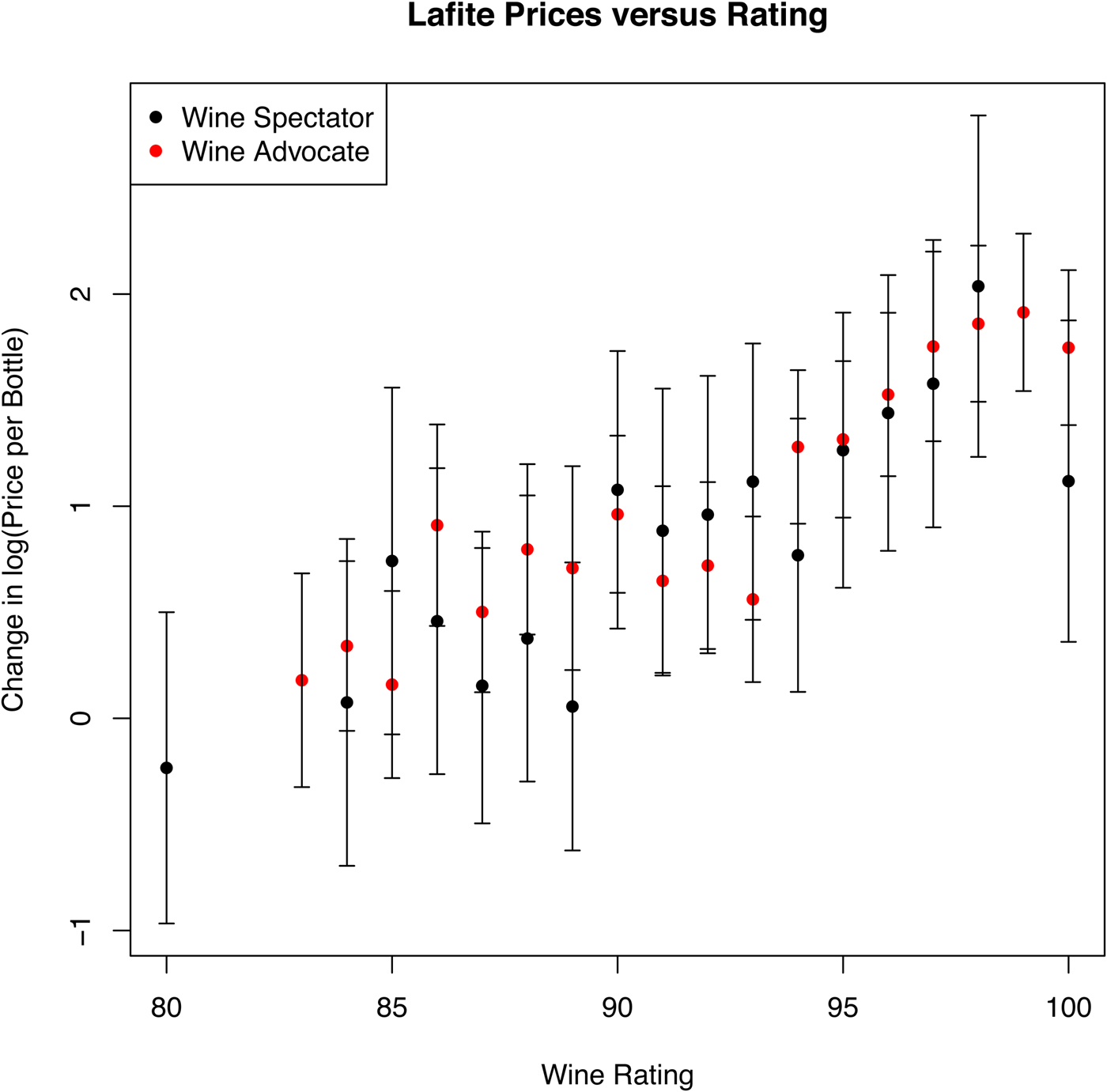
Figure 10 Change in Log-Price for Lafite Versus Wine Ratings after Normalizing for Life Cycle, Environment, Bottle Size, and Seller
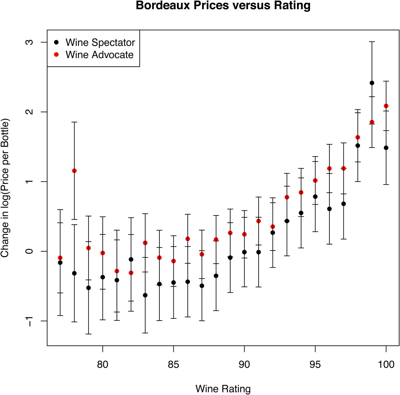
Figure 11 Change in Log-Price for Bordeaux Versus Wine Ratings after Normalizing for Life Cycle, Environment, Bottle Size, and Seller
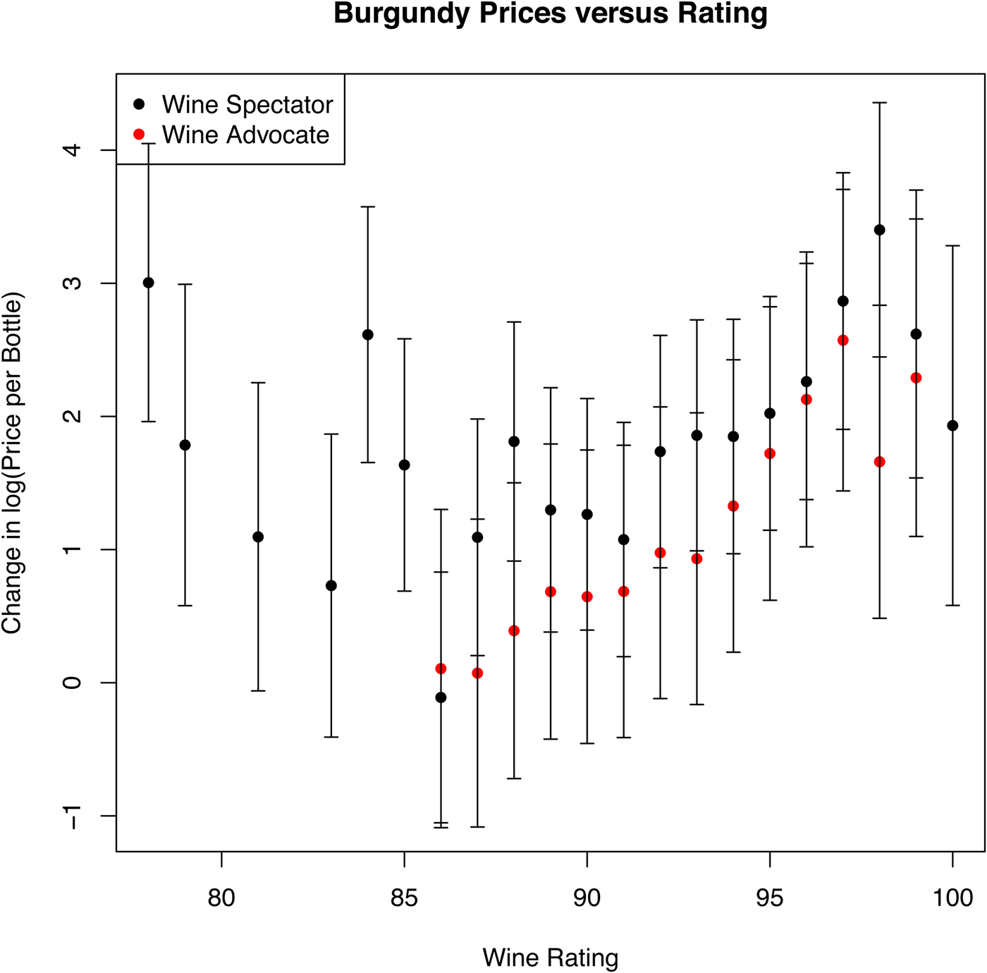
Figure 12 Change in Log-Price for Burgundy Versus Wine Ratings after Normalizing for Life Cycle, Environment, Bottle Size, and Seller
Cardebat, Figuet, and Paroissien (Reference Cardebat, Figuet and Paroissien2014) perform an analysis of wine ratings in combination with weather and other factors, using a series of regression models. Their analysis also incorporates a linear function of the wine's age. Their interesting results indicate that wine ratings are partially predictable from these external factors, but they also directly estimate the value of the ratings as a linear function when predicting log price. They estimate that for Wine Advocate, a 1-point increase in the experts’ opinion has a maximum impact of 4.1%. Although intuitively in agreement with this result, we find that the relationship is quite nonlinear, as shown in Figure 11. In general, one of the biggest advantages of our analysis is that all relationships are fully nonlinear, as further evidenced when comparing the life-cycle function here to the linear functions of age often found in previous analyses.
C. Auction Houses
Lastly, we study the importance of auction houses. With nine auction houses in the study, we measure the distribution of prices separately again for Lafite, Bordeaux excluding Lafite, and Burgundy, as shown in Figure 13. In all cases, the scaling coefficients by auction house are statistically significant, meaning that auction houses are a useful predictive factor for price. For Lafite and Bordeaux excluding Lafite, the price spread is one-third of an order of magnitude – a large number in dollar terms. For Burgundy, the spread is even higher, at 1.4 orders of magnitude in price.

Figure 13 Distribution of Price Adjustments by Auction House
To further confirm the distribution of price deltas by auction house, Figure 14 shows the price deltas of Burgundy versus Bordeaux, with each point representing one auction house. Although Burgundy has a greater price spread than Bordeaux, the results are highly correlated. Auction houses obtaining the highest prices for Bordeaux also get the highest prices for Burgundy, and vice versa.

Figure 14 Correlation Between Auction-House Price Deltas for Bordeaux and Burgundy
As before, the effect is statistically significant and normalized for all prior effects (wine age, specific wine pricing, market conditions, and unit sizes). However, the causality is open to interpretation. Wine history and condition are not included in the analysis, so it could be that certain auction houses only carry wines of better provenance. Conversely, it could be that the wines are the same, but auction house brand and participation account for the higher prices.
VII. Conclusion
This study seeks to provide new insights from an analytical perspective and by analyzing a dataset with unusual breadth. For the analytics, the APC algorithm and subsequent DTSM analysis with life cycle and environment as inputs replicate the features of previous hedonic analysis while also connecting to the APC literature and refinements on treatment and interpretation of linear trends in age, vintage, and time. We believe that imprecise treatment of the linear-trend issue could have led to the variety of results reported in previous studies, especially where those studies analyze shorter time periods.
When applying these techniques to the auctionforecast.com database, we obtain several useful results. The prices-appreciation rate versus age of the vintage confirm previous results, but the nonlinear functions obtained in this study exhibit additional details in comparison to previous studies. Measures of the wine-market index (environment function) span a broader set of wines than previous studies. Those indices for Lafite and Bordeaux excluding Lafite confirm the “Lafite Bubble” (which is more generally a Bordeaux Bubble) and the existence of correlations with the Chinese market during that period, suggesting the influence of Chinese buyers.
Vintage analysis and subsequent detailed study of lot size, bottle size, wine rating, and auction house produce several useful results. Prices are efficient with respect to lot size (not considering possible cross-term effects with lot sequencing) but significantly inefficient with respect to bottle size. The relationship between wine ratings and vintage price appreciation is confirmed, but with significant nonlinear details added. Lastly, by looking across nine different auction houses, we observe a significant spread in wine prices, which we confirm by comparing the same measure for Lafite, Bordeaux excluding Lafite, and Burgundy.
By modeling auction price, the natural application is to wine investment. The overall conclusion from this analysis is that wines do appreciate in value over multiple decades, but the rate of appreciation for Lafite, Bordeaux excluding Lafite, and Burgundy is not great enough in itself for most investors. However, the life cycles show that buying and selling at the right points in the wines’ ages are important for maximizing return. Also, wine markets have shown significant volatility over the last decade, which is beneficial for those seeking to trade wines. This volatility is great enough that large profits are possible if one can effectively time the market.
As the auctionforecast.com database grows, this analysis can be expanded to other wines, such as Italian, Australian, and so forth. In addition, we hope to add factors descriptive of the wines’ conditions.


