INTRODUCTION
Altitudinal gradients in the tropics can provide an excellent natural laboratory for examining the long-term interactions between forest ecosystems and environmental parameters, and for understanding ecosystem responses to environmental change (Malhi et al. Reference MALHI, SILMAN, SALINAS, BUSH, MEIR and SAATCHI2010). It has long been observed that forest above-ground biomass tends to decrease with altitude in the tropics (Crews et al. Reference CREWS, KITAYAMA, FOWNES, RILEY, HERBERT, MULLER-DUBOIS and VITOUSEK1995, Delaney et al. Reference DELANEY, BROWN, LUGO, TORRES-LEZAMAA and BELLO QUINTEROA1997, Herbert & Fownes Reference HERBERT and FOWNES1999, Leuschner et al. Reference LEUSCHNER, MOSER, BERTSCH, RÖDERSTEIN and HERTEL2007), and more recently a number of studies have demonstrated that above-ground net primary productivity (NPP, the rate of growth of wood and canopy biomass) also tends to decrease with altitude (Girardin et al. Reference GIRARDIN, MALHI, MAMANI, HUARACA HUASCO, DURAND, FEELEY, RAPP, SILVA-ESPEJO, SILMAN, SALINAS and WHITTAKER2010, Reference GIRARDIN, SILVA-ESPEJO, DOUGHTY, HUARACA-HUASCO, METCALFE, GALIANO-CABRERA, DURAND-BACA, ARAGÃO, MARTHEWS, HUARACA-QUISPE, ALZAMORA-TAYPE, EGUILUZ-MORA, FARFÁN-AMÉZQUITA, GARCÍA-CABRERA, HALLADAY, FISHER, SILMAN, MEIR, SALINAS and MALHI2014; Huaraca Huasco et al. Reference HUARACA HUASCO, GIRARDIN, DOUGHTY, METCALFE, DURAND, SILVA-ESPEJO, GALIANO CABRERA, ARAGÃO, ROZAS DAVILA, MARTHEWS, HUARACA-QUISPE, ALZAMORA-TAYPE, EGUILUZ-MORA, FARFAN, CABRERA, HALLADAY, SALINAS-REVILLA, SILMAN, MEIR and MALHI2014, Kitayama & Aiba Reference KITAYAMA and AIBA2002, Moser et al. Reference MOSER, RÖDERSTEIN, SOETHE, HERTEL, LEUSCHNER, Beck, Bendix, Kottke, Makeschin and Mosandl2008, Raich Reference RAICH1997, Röderstein et al. Reference RÖDERSTEIN, HERTEL and LEUSCHNER2005, Soethe et al. Reference SOETHE, WILCKE, HOMEIER, LEHMANN, ENGELS, Beck, Bendix, Kottke, Makeschin and Mosandl2008, Tanner Reference TANNER1980). The reason for this decline remains the subject of a long-standing debate, with suggested drivers being temperature effects on plant metabolism or on nutrient cycling, low light levels in tropical montane cloud forests (TMCF) and soil waterlogging (Bruijnzeel & Veneklaas Reference BRUIJNZEEL and VENEKLAAS1998, Bruijnzeel et al. Reference BRUIJNZEEL, WATERLOO, PROCTOR, KUITERS and KOTTERINK1993, Grubb Reference GRUBB1977, Kitayama & Aiba Reference KITAYAMA and AIBA2002, Schuur & Matson Reference SCHUUR and MATSON2001, Tanner et al. Reference TANNER, VITOUSEK and CUEVAS1998, Vitousek & Sanford Reference VITOUSEK and SANFORD1986).
Although the absolute value of mean annual NPP has now been quantified for a number of tropical lowland and montane sites, no study to date has examined the patterns of NPP seasonality across multiple sites, and in particular along environmental gradients. Describing and quantifying such patterns can help understand the nature and importance of seasonality in tropical forest ecosystems.
The effects of long-term changes in the seasonality of temperature, rainfall and cloud cover on tropical lowland and montane forests are potentially very significant, but remain poorly understood (Collins et al. Reference COLLINS, KNUTTI, ARBLASTER, DUFRENSE, FICHEFET, FRIEDLINGSTEIN, GAO, GUTWOSKI, JOHNS, KRINNER, SHONGWE, TEBALDI, WEAVER, WHENER, Stocker, Quin, Plattner, Tignor, Allen, Boschung, Nauels, Xia, Bex and Midgley2013, Huaraca Huasco et al. Reference HUARACA HUASCO, GIRARDIN, DOUGHTY, METCALFE, DURAND, SILVA-ESPEJO, GALIANO CABRERA, ARAGÃO, ROZAS DAVILA, MARTHEWS, HUARACA-QUISPE, ALZAMORA-TAYPE, EGUILUZ-MORA, FARFAN, CABRERA, HALLADAY, SALINAS-REVILLA, SILMAN, MEIR and MALHI2014, Rapp & Silman Reference RAPP and SILMAN2012). Recent field and remote-sensing studies in lowland Amazonian forests suggest that the NPP of humid Amazonian forests may synchronize to seasonal variation in solar irradiance, whereas NPP of drier Amazonian forests synchronizes to seasonal variation in water supply (Chave et al. Reference CHAVE, NAVARRETE, ALMEIDA, ALVAREZ, ARAGÃO, BONAL, CHATELET, SILVA-ESPEJO, GORET, VON HILDEBRAND, JIMÉNEZ, PATIÑO, PEÑUELA, PHILLIPS, STEVENSON and MALHI2010, Myneni et al. Reference MYNENI, YANG, NEMANI, HUETE, DICKINSON, KNYAZIKHIN, DIDAN, FU, NEGRÓN JUÁREZ, SAATCHI, HASHIMOTO, ICHII, SHABANOV, TAN, RATANA, PRIVETTE, MORISETTE, VERMOTE, ROY, WOLFE, FRIEDL, RUNNING, VOTAVA, EL-SALEOUS, DEVADIGA, SU and SALOMONSON2007, Rapp & Silman Reference RAPP and SILMAN2012, Wright & van Schaik Reference WRIGHT and VAN SCHAIK1994).
In this paper we present the first detailed study (to our knowledge) of how the seasonality of the components of above-ground NPP varies with elevation, along a 2800-m altitudinal gradient in the Peruvian Andes. We hypothesize that solar irradiance is the primary driver of canopy phenology in cloudier high-elevation sites, whereas precipitation drives phenology in drier systems. We address the following specific hypothesis: (1) the amplitude and phase of seasonal variation of solar irradiance and precipitation vary along the altitudinal gradient; (2) the partitioning of above-ground NPP between wood, leaves, flowers and fruit shows no variation with altitude; (3) the seasonal variation of above-ground NPP is synchronized with the seasonality of solar irradiance in cloudier sites, and synchronized with precipitation in sites that experience a dry season.
MATERIALS AND METHODS
Site description
Our study region is the focus of the interdisciplinary Andes Biodiversity and Ecosystem Research Group (Malhi et al. Reference MALHI, SILMAN, SALINAS, BUSH, MEIR and SAATCHI2010). Eight experimental sites were established in 2006 from 1527 m to 3045 m asl on the eastern slope of the Andes, in the Kosñipata valley, Province of Paucartambo, Department of Cusco, Southern Peruvian Andes, one site was established at 1000 m in an adjacent valley (Tono valley), a further two lowland Amazonian sites (215 m and 223 m asl) were established in the Tambopata reserve, Tambopata Province, Department of Madre de Dios, Peru, approximately 244 km east of the main transect, and two lowland Amazonian sites (120 m and 150 m asl) were established in the Maynas Province, Department of Loreto, Peru, within the Allpahuayo-Mishana National Reserve. All sites were monitored according to the same protocol. Four plots were continuously monitored from 2006 to 2011, five were monitored from 2006 to 2008 and a further two plots were established in 2008 and monitored until 2011 (Appendix 1).
Girardin et al. (Reference GIRARDIN, MALHI, MAMANI, HUARACA HUASCO, DURAND, FEELEY, RAPP, SILVA-ESPEJO, SILMAN, SALINAS and WHITTAKER2010) reported annual NPP estimates for a number of these sites. More recently, Girardin et al. (Reference GIRARDIN, SILVA-ESPEJO, DOUGHTY, HUARACA-HUASCO, METCALFE, GALIANO-CABRERA, DURAND-BACA, ARAGÃO, MARTHEWS, HUARACA-QUISPE, ALZAMORA-TAYPE, EGUILUZ-MORA, FARFÁN-AMÉZQUITA, GARCÍA-CABRERA, HALLADAY, FISHER, SILMAN, MEIR, SALINAS and MALHI2014), Huaraca Huasco et al. (Reference HUARACA HUASCO, GIRARDIN, DOUGHTY, METCALFE, DURAND, SILVA-ESPEJO, GALIANO CABRERA, ARAGÃO, ROZAS DAVILA, MARTHEWS, HUARACA-QUISPE, ALZAMORA-TAYPE, EGUILUZ-MORA, FARFAN, CABRERA, HALLADAY, SALINAS-REVILLA, SILMAN, MEIR and MALHI2014), Malhi et al. (Reference MALHI, AMEZQUITA, DOUGHTY, SILVA-ESPEJO, GIRARDIN, METCALFE, ARAGAO, HUARACA-QUISEPE, ALZAMORA-TAYPE, EGUILUZ-MORA, MARTHEWS, HALLADAY, QUESADA, ROBERTSON, FISHER, ZARAGOZA-CASTELLS, ROJAS-VILLAGRA, PELAEZ-TAPIA, SALINAS, MEIR and PHILLIPS2014) and del Aguila-Pasquel et al. (Reference DEL AGUILA-PASQUEL, DOUGHTY, METCALFE, SILVA-ESPEJO, GIRARDIN, CHUNG GUTIERREZ, NAVARRO-AGUILAR, QUESADA, HIDALGO, REYNA HUAYMACARI, HALLADAY, DEL CASTILLO TORRES, PHILLIPS and MALHI2014) provided comprehensive descriptions of the carbon cycle for eight of these sites.
As geological substrate and topographic position can have a significant influence on forest dynamics (Takyu et al. Reference TAKYU, AIBA and KITAYAMA2002), all the TCMF plots were established along a ridge-top on umbrisols, with a thick humic layer increasing in depth from 5 to 30 cm along the altitudinal gradient (B. Quesada, pers. comm.). The montane forest plots are situated on a bedrock of Palaeozoic slates and shales, with the exception of TU-07 and TU-08, situated on a late-Permian granite intrusion bedrock. Plots at 1000 m and below were situated on clay-rich sediments formed from alluvial deposition (though all are now above river flood levels). Total soil nitrogen and available phosphorus in the TMCF sites were above the range typically reported for lowland rain forests (B. Quesada, pers. comm.). Soil carbon, nitrogen and phosphorus stocks in the top 50 cm were highest in the 2000–3045-m band, where there was a build-up of a thick layer of humic material (typically 20–30 cm thick) above carbon-rich topsoil (Girardin et al. Reference GIRARDIN, SILVA-ESPEJO, DOUGHTY, HUARACA-HUASCO, METCALFE, GALIANO-CABRERA, DURAND-BACA, ARAGÃO, MARTHEWS, HUARACA-QUISPE, ALZAMORA-TAYPE, EGUILUZ-MORA, FARFÁN-AMÉZQUITA, GARCÍA-CABRERA, HALLADAY, FISHER, SILMAN, MEIR, SALINAS and MALHI2014).
All plots along the altitudinal transect were selected in areas with relatively homogeneous stand structure, and with no sign of significant human influence. All had closed canopies without any large gaps, although lowland forests have less gaps and a more even canopy than TMCF forests. Forest composition changed with altitude: the most common families in the lowland plots were Clusiaceae, Bixaceae, Urticaceae, Moraceae and Fabaceae; lower montane plots were dominated by the families Sapotaceae, Moraceae, Clusiaceae, Urticaceae, Euphorbiaceae and Anacardiaceae, and the highest altitudinal plots were dominated by Clusiaceae, Cunoniaceae, Sabiaceae, Rosaceae and Lauraceae (Appendix 1). Species composition varied considerably between neighbouring plots, with likely impacts on productivity. At highest altitudes, the 3045-m stand (Wayqecha) was dominated by Weinmannia crassifolia and a number of successsional species (e.g. Pentacalia spp., Ageratina spp. and Hesperomeles ferruginea).
Weather data
Time series for solar irradiance (W m−2), air temperature (°C), relative humidity (%) and precipitation (mm mo−1) were collected from Automatic Weather Stations (AWS, Campbell Scientific) located c. 1 km from the 3045-, 1527- and 215-m stands (Halladay et al. Reference HALLADAY, NEW and MALHI2012). The original data were measured with at least 30-min resolution for the period July 2005 to December 2010. These data were quality controlled to remove outliers, and monthly time series were gap-filled as described in Girardin et al. (Reference GIRARDIN, SILVA-ESPEJO, DOUGHTY, HUARACA-HUASCO, METCALFE, GALIANO-CABRERA, DURAND-BACA, ARAGÃO, MARTHEWS, HUARACA-QUISPE, ALZAMORA-TAYPE, EGUILUZ-MORA, FARFÁN-AMÉZQUITA, GARCÍA-CABRERA, HALLADAY, FISHER, SILMAN, MEIR, SALINAS and MALHI2014).
The transition from lower to upper montane forest often coincides with more persistent dry-season cloud condensation (Bruijnzeel Reference BRUIJNZEEL2004, Edwards & Grubb Reference EDWARDS and GRUBB1977, Hamilton et al. Reference HAMILTON, JUVIK, SCATENA, Bruijnzeel, Scatena and Hamilton1995). We do not have sufficient meteorological data to determine the altitudinal limits of the cloud immersion zone in the Kosñipata valley. Nonetheless, based on forest composition (e.g. large increase in vascular epiphyte and bryophyte biomass, Horwath Reference HORWATH2011), soil properties (Zimmermann et al. Reference ZIMMERMANN, MEIR, BIRD, MALHI and CCAHUANA2009) and the ecophysiology (Girardin et al. Reference GIRARDIN, MALHI, MAMANI, HUARACA HUASCO, DURAND, FEELEY, RAPP, SILVA-ESPEJO, SILMAN, SALINAS and WHITTAKER2010) of forests along the Kosñipata Valley, we estimate that the base of the cloud zone forms between 1527 and 1800 m asl (J. Rapp, pers. comm.).The cloud-forest zone extends to the tree line at approximately 3400 m asl, above which puna grasslands dominate (Halladay et al. Reference HALLADAY, NEW and MALHI2012).
Net primary productivity
Above-ground coarse woody net primary productivity
We determined plot-level NPPACW using multiple censuses (2003, 2007, 2011) of the forest plots and three-monthly dendrometer band measurements (November 2006–September 2011). We completed tree censuses to determine the growth rate of existing surviving trees and the rate of recruitment of new trees. Data on dbh (diameter tape) and tree height (clinometer when possible, or visual estimate) were recorded for all trees ≥ 10 cm dbh. Mortality in any year was estimated for each site by calculating the biomass of trees that were measured alive in the previous annual census and were dead in the latest census. ACW biomass was calculated using the allometric equation of Chave et al. (Reference CHAVE, ANDALO, BROWN, CAIRNS, CHAMBERS, EAMUS, FÖLSTER, FROMARD, HIGUCHI, KIRA, LESCURE, NELSON, OGAWA, PUIG, RIÉRA and YAMAKURA2005) for tropical moist forests, employing data on diameter, height and wood density.
where AGB is above-ground biomass (kg), ρ is density of wood (g cm−3), dbh is diameter at breast height (cm) and H is height (m). Wood density was estimated for each species from a global database of tropical forest wood density (Chave et al. Reference CHAVE, COOMES, JANSEN, LEWIS, SWENSON and ZANNE2009), ideally assigned to species, but to genus or family level where species identity or species-level wood-density data were not available. To convert biomass values into carbon, we assumed that dry ACW biomass is 47.3% carbon, based on recent studies in lowland forests in Panama that included volatile carbon compounds not recorded by conventional dry assessment (Martin & Thomas Reference MARTIN and THOMAS2011). For the few trees where height data were not available we estimated height by employing a plot-specific polynomial regression between dbh and height. Tree fern incidence ranged from 0% in the lowlands to 21% at 2020 m, peaking between 1885 m and 2758 m asl. Palm tree incidence varied from 0% (3045 m) to 27% in one plot in the Tambopata lowlands. The biomass was then summed over all trees > 10 cm dbh to estimate total above-ground biomass. Above-ground woody production was calculated as the sum of biomass increase of individual surviving trees between census intervals.
To determine seasonal variation in woody growth rates, we installed dendrometer bands in January 2007 or 2009 (Appendix 1) on approximately 200 randomly selected trees in each plot (all trees in Tambopata lowland plots). The 200 dendrometer bands were measured every 3 mo with callipers. The dendrometer data were scaled up to 1 ha by using the annual full census data to determine the ratio of wood net primary productivity (NPP ACW) of all trees over NPP ACW of dendrometer trees. This ratio provided a scaling factor that we applied to the dendrometer data, to estimate seasonal NPP ACW for the entire plot (i.e. to include trees that had no dendrometers), with the implicit assumption that the productivity of the dendrometer trees is representative of the wider population. The effects of seasonal moisture expansion on tree growth data were estimated to be negligible, based on examination of seasonal diameter variation of slow-growing trees (Girardin et al. Reference GIRARDIN, SILVA-ESPEJO, DOUGHTY, HUARACA-HUASCO, METCALFE, GALIANO-CABRERA, DURAND-BACA, ARAGÃO, MARTHEWS, HUARACA-QUISPE, ALZAMORA-TAYPE, EGUILUZ-MORA, FARFÁN-AMÉZQUITA, GARCÍA-CABRERA, HALLADAY, FISHER, SILMAN, MEIR, SALINAS and MALHI2014, Huaraca Huasco et al. Reference HUARACA HUASCO, GIRARDIN, DOUGHTY, METCALFE, DURAND, SILVA-ESPEJO, GALIANO CABRERA, ARAGÃO, ROZAS DAVILA, MARTHEWS, HUARACA-QUISPE, ALZAMORA-TAYPE, EGUILUZ-MORA, FARFAN, CABRERA, HALLADAY, SALINAS-REVILLA, SILMAN, MEIR and MALHI2014, Malhi et al. Reference MALHI, AMEZQUITA, DOUGHTY, SILVA-ESPEJO, GIRARDIN, METCALFE, ARAGAO, HUARACA-QUISEPE, ALZAMORA-TAYPE, EGUILUZ-MORA, MARTHEWS, HALLADAY, QUESADA, ROBERTSON, FISHER, ZARAGOZA-CASTELLS, ROJAS-VILLAGRA, PELAEZ-TAPIA, SALINAS, MEIR and PHILLIPS2014). As the census interval was small (1 y) we did not apply a correction for trees that grow and die between census intervals without being recorded (Malhi et al. Reference MALHI, BAKER, PHILLIPS, ALMEIDA, ALVAREZ, ARROYO, CHAVE, CZIMCZIK, DI FIORE, HIGUCHI, KILLEEN, LAURANCE, LAURANCE, LEWIS, MERCADO MONTOYA, MONTEAGUDO, NEILL, VARGAS, PATIÑO, PITMAN, QUESADA, SALOMÃO, SILVA, LEZAMA, MARTÍNEZ, TERBORGH, VINCETI and LLOYD2004). We did not account for the wood productivity of lianas in Tambopata, although their leaf productivity is recorded by litterfall traps.
Litterfall
Canopy litterfall was collected in 25 0.25-m2 (50 × 50 cm) litter traps installed 1 m above the ground on each plot. There were only five litter traps at 2020 m asl due to topographic constraints. Litterfall was collected every 15 d over a period of 18 or 24 mo between 2006 and 2011 (Appendix 1), split into different components (leaves, fruits, flowers, seeds, woody tissue, bromeliads, other epiphytes (non-vascular epiphytes, mosses and liverworts) and unidentified fine debris), oven dried at 80 ºC, and weighed. Seasonal variation of large palm leaf litter was not accounted for in the lowland plots, implying an underestimation of litterfall at 215 m and at 223 m asl. Malhi et al. (Reference MALHI, AMEZQUITA, DOUGHTY, SILVA-ESPEJO, GIRARDIN, METCALFE, ARAGAO, HUARACA-QUISEPE, ALZAMORA-TAYPE, EGUILUZ-MORA, MARTHEWS, HALLADAY, QUESADA, ROBERTSON, FISHER, ZARAGOZA-CASTELLS, ROJAS-VILLAGRA, PELAEZ-TAPIA, SALINAS, MEIR and PHILLIPS2014) estimate that palm leaf litterfall accounts for 5.46% ± 0.12% (TAM-05) and 75.7% ± 0.11% (TAM-06) of total leaf litterfall in the two lowland plots.
Litterfall is a good estimator of canopy productivity on annual or larger timescales. However, it represents the timing of canopy biomass loss, not biomass gain, and hence cannot record seasonal variation in canopy productivity. We combined datasets of litterfall, canopy Leaf Area Index, LAI (del Aguila-Pasquel et al. Reference DEL AGUILA-PASQUEL, DOUGHTY, METCALFE, SILVA-ESPEJO, GIRARDIN, CHUNG GUTIERREZ, NAVARRO-AGUILAR, QUESADA, HIDALGO, REYNA HUAYMACARI, HALLADAY, DEL CASTILLO TORRES, PHILLIPS and MALHI2014, Girardin et al. Reference GIRARDIN, SILVA-ESPEJO, DOUGHTY, HUARACA-HUASCO, METCALFE, GALIANO-CABRERA, DURAND-BACA, ARAGÃO, MARTHEWS, HUARACA-QUISPE, ALZAMORA-TAYPE, EGUILUZ-MORA, FARFÁN-AMÉZQUITA, GARCÍA-CABRERA, HALLADAY, FISHER, SILMAN, MEIR, SALINAS and MALHI2014, Huaraca Huasco et al. Reference HUARACA HUASCO, GIRARDIN, DOUGHTY, METCALFE, DURAND, SILVA-ESPEJO, GALIANO CABRERA, ARAGÃO, ROZAS DAVILA, MARTHEWS, HUARACA-QUISPE, ALZAMORA-TAYPE, EGUILUZ-MORA, FARFAN, CABRERA, HALLADAY, SALINAS-REVILLA, SILMAN, MEIR and MALHI2014, Malhi et al. Reference MALHI, AMEZQUITA, DOUGHTY, SILVA-ESPEJO, GIRARDIN, METCALFE, ARAGAO, HUARACA-QUISEPE, ALZAMORA-TAYPE, EGUILUZ-MORA, MARTHEWS, HALLADAY, QUESADA, ROBERTSON, FISHER, ZARAGOZA-CASTELLS, ROJAS-VILLAGRA, PELAEZ-TAPIA, SALINAS, MEIR and PHILLIPS2014) and Specific Leaf Area, SLA (Salinas et al. Reference SALINAS, MALHI, MEIR, SILMAN, ROMAN CUESTA, HUAMAN, SALINAS, HUAMAN, GIBAJA, MAMANI and FARFAN2011) to estimate the seasonal cycle of canopy net primary productivity (NPP canopy) at low (~200 m), mid- (~1527 m) and high (~3000 m) altitudes (Doughty & Goulden Reference DOUGHTY and GOULDEN2008):
where ΔLAI is the change in LAI between months (m2 m−2), SLA is the mean specific leaf area (m2 g−1) and litterfall is total litterfall (g m−2). We estimate SLA by taking a subsample of fresh leaf litterfall, scanning each leaf to determine fresh leaf area, and then drying at 80 °C and weighing the leaf to determine dry mass. SLA is fresh leaf area divided by dry leaf mass. Leaf area was calculated using image analysis software, Image J freeware (http://rsb.info.nih.gov/ij/). NPP canopy is estimated in g m−2.
Above-ground net primary productivity. NPP AG can be estimated as the sum of NPP ACW, NPP canopy, branch turnover (NPP branch turnover) and volatile organic compound production (NPP VOC).
 \begin{eqnarray}
\textit{NPP}_{{\rm AG}} &=& \textit{NPP}_{{\rm ACW}} + \textit{NPP}{\rm canopy} \nonumber\\
&&+\, \textit{NPP}_{{\rm branch}} \,_{{\rm turnover}} + \textit{NPP}_{{\rm VOC}}\end{eqnarray}
We obtained seasonal NPP ACW estimates from the dendrometer band growth, and NPP canopy values through the seasonal litterfall measurements coupled with seasonal variation in Leaf Area Index. Branch turnover productivity is hard to estimate at seasonal resolution (Girardin et al. Reference GIRARDIN, SILVA-ESPEJO, DOUGHTY, HUARACA-HUASCO, METCALFE, GALIANO-CABRERA, DURAND-BACA, ARAGÃO, MARTHEWS, HUARACA-QUISPE, ALZAMORA-TAYPE, EGUILUZ-MORA, FARFÁN-AMÉZQUITA, GARCÍA-CABRERA, HALLADAY, FISHER, SILMAN, MEIR, SALINAS and MALHI2014, Huaraca-Huasco et al. Reference HUARACA HUASCO, GIRARDIN, DOUGHTY, METCALFE, DURAND, SILVA-ESPEJO, GALIANO CABRERA, ARAGÃO, ROZAS DAVILA, MARTHEWS, HUARACA-QUISPE, ALZAMORA-TAYPE, EGUILUZ-MORA, FARFAN, CABRERA, HALLADAY, SALINAS-REVILLA, SILMAN, MEIR and MALHI2014), hence for the purpose of this paper, we concentrate on NPP ACW and NPP canopy seasonality. Finally, we did not estimate the contribution of volatile organic carbon emission from vegetation, which was found to be a very minor contribution in lowland tropical forest ecosystems (Malhi et al. Reference MALHI, ARAGÃO, METCALFE, PIVA, QUESADA, ALMEIDA, ANDERSON, BRANDO, CHAMBERS, DA COSTA, HUTYRA, OLIVIERA, PATINO, PYLE, ROBERTSON and TEIXEIRA2009).
Analytical techniques
We used these data to describe the seasonal variation of NPP ACW and litterfall along the Kosñipata altitudinal gradient. All uncertainty estimates are given as the standard error of the mean. Linear regression analyses were conducted to identify significant altitudinal trends in ecosystem allocation to above-ground components of productivity and the relationships between components. We used stepwise regression to explore the correlations between abiotic parameters and NPP ACW. We explored the seasonal amplitude of each abiotic and biotic parameter. Seasonal amplitude was estimated by subtracting the minimum 3-mo moving average from the maximum moving average recorded. Repeated-measures ANOVA was used to assess the significance of seasonal increases in productivity. All error estimates are provided as ± SE. All statistical analyses were performed with the R version 2.9.0 statistical package (Chambers Reference CHAMBERS2008).
RESULTS
How do the amplitude and phase of seasonal variation of solar irradiance and precipitation vary along the altitudinal gradient?
Annual means
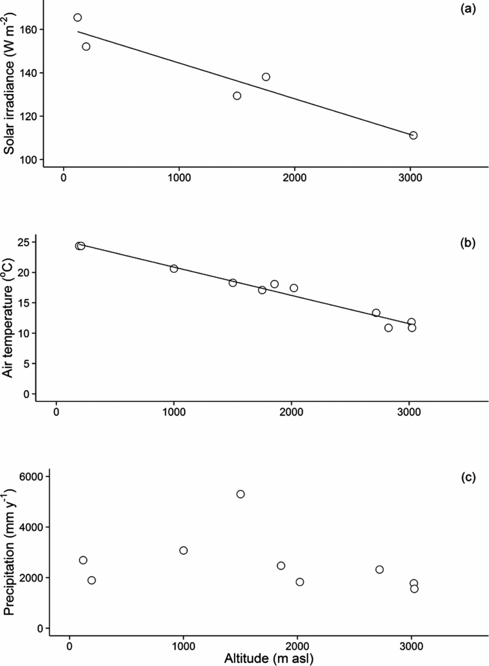
Over the study period, mean annual air temperatures ranged from 24.9 ºC ± 1.06 ºC (223 m asl) to 10.9 ºC ± 0.44 ºC (3045 m asl). A linear regression against altitude explained 97% of the variation in mean air temperature (P < 0.0001), with an air temperature lapse rate of 4.69 ºC km−1 along the transect (Figure 1). Mean annual rainfall varied between 5302 mm y−1 below the cloud base (1527–1776 m asl) and 1560 mm y−1 at the highest altitude (3045 m asl), this may be lower than long-term means as the region experienced droughts during the study period, in 2005 and 2010. Neither water shortage nor prolonged water logging were recorded in the TMCF sites. Mean annual shortwave irradiance decreased significantly as cloud amount increased with altitude, from 4.8 GJ m−2 y−1 at 215 m asl to 3.51 GJ m−2 y−1 at 3045 m asl.

Figure 1. Weather patterns along the Kosñipata altitudinal gradient, Peruvian Andes. Solar irradiance (W m−2, r2 = 0.94, P < 0.001) (a), mean annual air temperature (ºC, SE < 0.05, r2 = 0.96, P < 0.0001) (b) and mean annual precipitation (c) are reported at each altitude. We provide data from Acjanaco (3950 m asl), a weather station located in the grassland above the treeline, although it is not a plot in this study. Error estimates are provided as ± SE.
Seasonality in solar irradiance
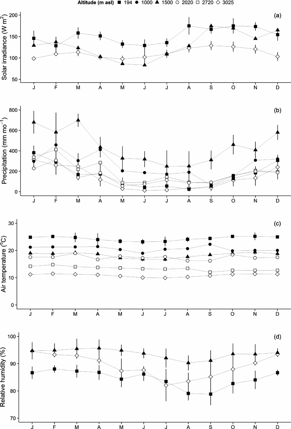
In the lowlands, light availability was fairly constant throughout the year, as lower sun angles offset the lower cloudiness of the dry season (austral winter). Seasonality of solar irradiance was most pronounced at TMCF sites: low sun angles, short days and a lower cloud base (resulting in more frequent cloud immersion) resulted in a decrease in solar irradiance during the austral winter. At all altitudes, solar irradiance increased towards the end of the dry season, reaching a peak between September and November, just before the dry-to-wet transition period. Although we did not obtain sufficient data to estimate the full seasonal cycle of solar irradiance at each altitude, the data we obtained from low-, mid- and high-altitude sites allowed us to record the seasonality of solar irradiance across the gradient (Figure 2a).

Figure 2. Seasonality of weather components along the Kosñipata altitudinal gradient, Peruvian Andes. Solar irradiance (W m−2) is reported at 3045 m, 1776 m, 1527 m and 215 m (a), precipitation (mm mo−1) at 3045 m, 2758 m, 1885 m, 1776 m, 1527 m and 215 m, air temperature (ºC) at 3045 m, 2758 m, 2020 m, 1885 m, 1776 m, 1527 m and 215 m, and relative humidity (%) at 3045 m, 1527 m and 215 m. Error estimates are provided as ± SE.
Precipitation
All sites showed strong seasonal variation of rainfall, with highest values recorded between December and February (Figure 2b). The dry season caused significant water deficits (precipitation <100 mm mo−1) at the lowland sites, and may also cause seasonal water stress at the top of the transect, near the treeline (although evapotranspiration rates are likely to be lower). The intermediate montane sites showed less seasonality in water availability and soil moisture content, with precipitation remaining fairly high in the dry season (lower montane sites) and/or cloud immersion suppressing water loss through evapotranspiration (upper montane sites). In the lowlands, the Allpahuayo sites (120 m asl and 150 m asl) had less seasonality in rainfall than other lowland Amazonian forests, with rainfall ranging from 100 mm mo−1 to 300 mm mo−1, and no dry season.
Air temperature
We found very little seasonal variation in air temperature along the altitudinal gradient (Figure 2c). Relative humidity shows moderate seasonality at the lowland and upper treeline ends of the transect (Figure 2d) in synchrony with the wet and dry seasons, but little seasonality at the intermediary montane sites, where cloud immersion is frequent in the dry season.
How does the partitioning of the components of NPP AG between wood, leaves, flowers and fruit vary with altitude?
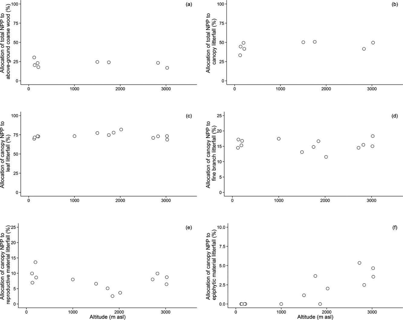
Total NPP AG has previously been shown to decline substantially with altitude for this transect (Girardin et al. Reference GIRARDIN, MALHI, MAMANI, HUARACA HUASCO, DURAND, FEELEY, RAPP, SILVA-ESPEJO, SILMAN, SALINAS and WHITTAKER2010). Strikingly, the allocation of the components of NPP AG show no trends with altitude. On average, the fraction of total NPP in the canopy is 45% ± 2%, and in above-ground coarse woody material is 23% ± 1%. The mean fraction of canopy NPP in flowers and fruit material is 8% ± 1%, and in fine wood (twig) production is 15% ± 0.5%. Epiphyte litter (probably significantly underestimated because much epiphyte material can decompose in situ) accounts for less than 2% ± 0.5% of litterfall in the montane cloud forests, but makes a negligible contribution to the lowland and submontane forests (Figure 3).

Figure 3. Allocation of total net primary productivity (NPP Total) to above-ground coarse wood (NPP ACW) (a) and canopy (NPP canopy) (b) productivity, and allocation of canopy net primary productivity (NPP canopy) to canopy components along the Kosñipata altitudinal gradient, Peruvian Andes. Annual canopy litterfall data are separated into allocation (%) to leaves (c), fine branch (d), reproductive material (flowers and fruit) (e) and epiphytic material (f) along the altitudinal gradient. Epiphytic material increases significantly with altitude (r2 = 0.69, P < 0.001).
How does the seasonal variation in the components of NPP AG vary with altitude?
Above-ground coarse woody net primary productivity
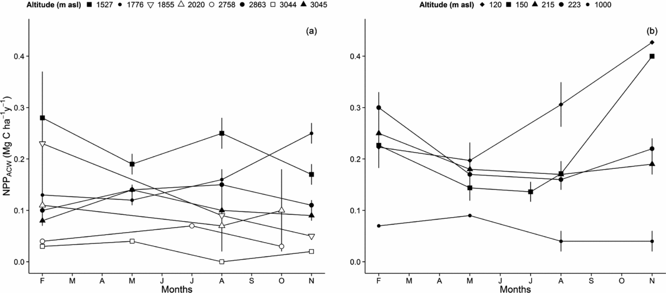
We recorded seasonal trends of NPP ACW at all altitudes (Figure 4). Forests located below the cloud base showed clear seasonal trends of NPP ACW, with significantly higher growth rates reported during the peak wet season, November–March (0.30 ± 0.03 Mg C ha−1 mo−1 at 215 m asl, 0.25 ± 0.02 Mg C ha−1 mo−1 at 223 m asl, 0.43 ± 0.06 Mg C ha−1 mo−1 at 120 m asl and 0.40 ± 0.06 Mg C ha−1 mo−1 at 150 m asl) and minimum growth rates during the peak dry season, May–August (0.16 ± 0.02 Mg C ha−1 mo−1 at 215 m asl, 0.17 ± 0.02 Mg C ha−1 mo−1 at 223 m asl, 0.20 ± 0.03 Mg C ha−1 mo−1 at 120 m asl and 0.14 ± 0.02 Mg C ha−1 mo−1 at 150 m asl). This is true even in the northern Peru Allpahuayo plots, where rainfall remains quite high in the dry season and there is little seasonal water stress. There was a weak inverse seasonality at the highest altitudes (2758 m to 3045 m), with a tendency to increase woody production during the months of lower rainfall.

Figure 4. Seasonal variation of above-ground woody productivity (NPP ACW) along the Kosñipata altitudinal gradient, Peruvian Andes. Data provided for Tropical Cloud Montane Forest Plots, at 3045 m, 3044 m, 2863 m, 2758 m, 2020 m, 1885 m, 1776 m, 1527 m (a), and plots located below the cloud base, at 1000 m, 215 m, 223 m, 120 m, 150 m (b). Error estimates are provided as ± SE.
Canopy net primary productivity
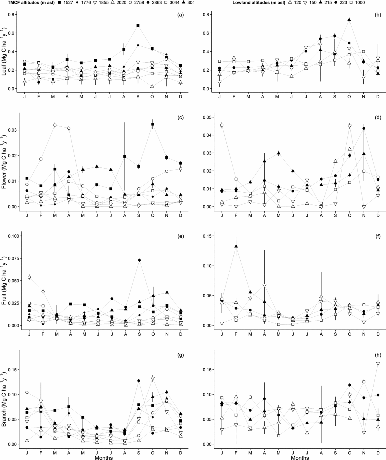
We monitored the seasonal variation in each component of canopy litterfall at each altitude. Within the cloud immersion zone, leaf litterfall showed almost no seasonality, with the notable exception of the cloud-base transition plot at 1500 m which shows a peak in litterfall in the late dry season (August–October), and to a lesser degree the higher transition plot at 1776 m (Figure 5a). Below the cloud base (~1500 m asl), the forest plots showed a strong peak in leaf litterfall rates (shedding) and synchronous production (replacement) through the mid and late dry season (August–October) (Figures 5b, 6).

Figure 5. Seasonal variation of canopy litterfall components along the Kosñipata altitudinal gradient, Peruvian Andes. Canopy components were separated into leaf (a, b), flower (c, d), fruit (e, f), and fine branch (g, h). Data provided for Tropical Cloud Montane Forest plots, at 3045 m, 3044 m, 2863 m, 2758 m, 2020 m, 1885 m, 1776 m, 1527 m, and below the cloud base, at 1000 m, 215 m, 223 m, 150 m, and 120 m. Error estimates are provided as ± SE.

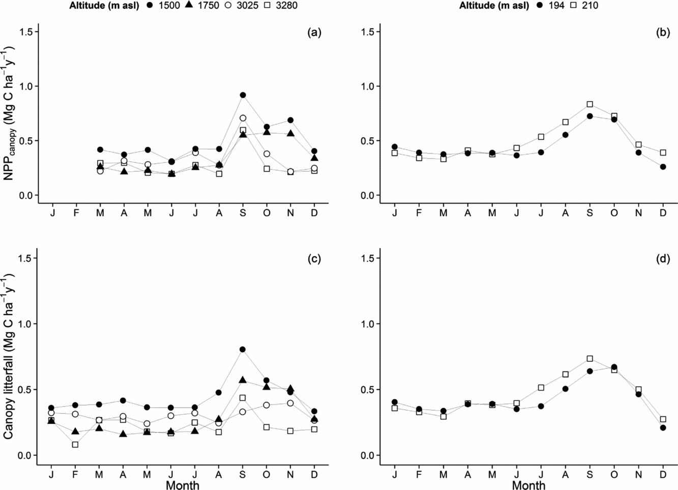
Figure 6. Seasonal variation of canopy net primary productivity (NPP canopy), compared with canopy litterfall along the Kosñipata altitudinal gradient, Peruvian Andes. NPP canopy seasonality was separated for plots within the tropical cloud montane forest (TMCF) sites (a) and below the cloud immersion zone (b). Canopy litterfall was also separated into TMCF plots (c) and low-altitude plots (d). TMCF plots were located at 3045 m, 2863 m, and 1776 m, 1527 m, and sites located below the cloud immersion zone were at 215 m and 223 m.
For a subset of our plots, we combined our leaf litterfall with monthly collected canopy leaf area data to estimate the seasonality in leaf production and compare with the seasonality of leaf litterfall (Figure 6). These analyses showed that the periods of leaf litterfall (August to November, late dry season and early wet season) synchronize with periods of leaf production, resulting in little seasonal variation in total canopy leaf area. In this study transect, the dominant trees appear to favour shedding and simultaneously renewing their leaves in the dry season, rather than having a period of reduced canopy leaf area. Such shedding and renewal occurs even in sites with little seasonal water stress (e.g. the very wet montane sites at 1500 and 1750 m asl), suggesting that leaf life cycle events are not driven by water stress.
The litterfall of twigs, flowers and fruits (Figure 5) showed a distinct seasonality at most altitudes, with a broad minimum over the austral winter (dry season, low cloud base with frequent cloud immersion in the mountains). In the lowlands and at the 1527-m transition site, flower litterfall peaks in October and November, before the onset of heavy wet-season rains. As most flowers only last for a few weeks before shedding, flower litterfall is likely a good indicator of seasonality in flower production.
In the TMCF, seasonal trends were strongest in the plots located at the lower (1527 m asl) and upper (2758 m asl) limits of the cloud immersion zone, with a bimodal peak mirroring those of solar irradiance. In the lowlands, all plots showed strong seasonality, with a period of increased flower fall at the start of the wet season, indicating a peak in flower production at the end of the dry season, when solar irradiance reaches its maximum values. Only the 215-m plot showed evidence of a bimodal peak in flower fall, at the start and at the end of the wet season.
Fruit litterfall showed no strong seasonality, but there was some evidence of a broad minimum during the dry season (May–July) and a broad maximum over the wet season (Figure 5e, f). This suggests fruit tended to develop in the few months after flowering (mid-late dry season), peaking in development in the early wet season. However, the fruitfall signal is smeared out by differing fruit development cycles between species, and possibly also by frugivory, which explains the less sharp patterns of seasonality in fruit fall.
Seasonal amplitude
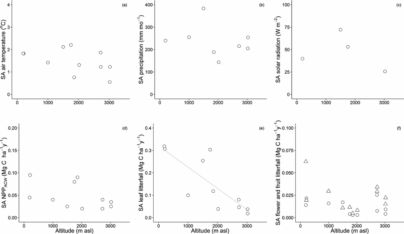
The seasonal amplitude of solar irradiance, precipitation and air temperature showed no significant trends along the altitudinal gradient. Of all components of NPP AG monitored, only leaf litterfall showed a significant decrease in seasonal amplitude with increasing altitude. The lowland sites showed more seasonality in leaf production, although this result partially reflected the higher absolute amounts of leaf production at these sites. The seasonal amplitude of NPP ACW and of the productivity of reproductive organs (estimated as flower and fruit litterfall) remained remarkably constant over the altitudinal gradient (Figure 7).

Figure 7. Seasonal Amplitude (SA) of weather components and above-ground components of net primary productivity along the Kosñipata altitudinal gradient, Peruvian Andes. SA of weather components are presented as air temperature (a), monthly precipitation (b) and solar irradiance (c). SA of all metrics or proxies for net primary productivity are provided in Mg C ha−1 y−1: above-ground coarse woody material (d), leaf litterfall (e), flower and fruit litterfall (f).
Is there any evidence of synchrony between the seasonal variation of productivity and the seasonality of light or precipitation, and does the pattern of synchrony vary with altitude?
NPPcanopy and solar irradiance
The seasonality of NPP canopy was in synchrony with the seasonality of solar irradiance at all sites. In most sites, the month of maximum NPP canopy was recorded 1–2 mo before the peak in rainfall, when solar irradiance was at its maximum.
NPPACW and precipitation
In the lowlands, we recorded an increase in the production of above-ground coarse woody material at the start of the wet season. There was no correlation between NPP ACW and precipitation in TMCF sites.
NPPflower, NPPfruit and solar irradiance
In wet forest sites, flowering patterns were in synchrony with the seasonal trends of solar irradiance. Flower litterfall peaked in October or November, implying that the increase in the production of flowers coincided with the increase in solar irradiance (September–November) at those sites. Two plots (1527 m asl and 2758 m asl) displayed a second peak in flowering that coincided with a secondary peak in solar irradiance (March).
DISCUSSION
Seasonal trends of above-ground net primary productivity
Drivers of NPPcanopy seasonality
The seasonality of NPP canopy appears to be in synchrony with solar irradiance and maintains this pattern even in plots with seasonal water stress, partially confirming hypothesis (3). This may be because trees optimize their resources to boost photosynthetic rates through new leaves at a time of high photosynthetically active radiation (PAR). An alternative hypothesis is that trees invest in building new leaves during the dry season, a period of lower relative humidity and therefore lower pathogen, fungal and insect herbivory pressure (Givnish Reference GIVNISH1999, Leigh Reference LEIGH and Leigh1999, Wright & van Schaik Reference WRIGHT and VAN SCHAIK1994).
Canopy litterfall as a proxy for NPPcanopy seasonality
The data presented in this study are unique in that we were able to track NPP canopy in terms of leaf flush and senescence, rather than relying solely on litterfall as a proxy for productivity. Litterfall is understood to be a reliable estimate of canopy productivity over annual timeframes in ecosystems in equilibrium, however, the relationship between litterfall and leaf production on a seasonal timescale in evergreen tropical forests has only recently been explored (Doughty & Goulden Reference DOUGHTY and GOULDEN2008).
We found that seasonality of canopy litterfall closely tracks seasonality of NPPcanopy at all sites, except Wayqecha (3045 m asl) (Figure 6). In most forests we monitored, the production of new leaves (leaf flush) matched the loss of senescent leaves over the seasonal cycle. This suggests that the dominant trees in most of our plots are leaf-exchangers rather than leaf shedders, and that this period of leaf exchange is optimized for the mid- to late dry season. It also suggests that leaf litterfall is a reasonable indicator of seasonality in leaf production, especially in our lower-altitude plots.
The upper montane plots show a distinct peak in NPP canopy in August, contrasting with a slow increase in litterfall. A decoupling of NPP canopy and litterfall patterns suggest that leaf flush exceeds leaf senescence. As a result, we observe an increase in LAI in August, after a peak in solar irradiance. This trend is most notable in Wayquecha. The species composition of Wayqecha, high NPP, low basal area, low incidence of large trees, high density of small-dbh stems and high recruitment rates (Girardin et al. Reference GIRARDIN, SILVA-ESPEJO, DOUGHTY, HUARACA-HUASCO, METCALFE, GALIANO-CABRERA, DURAND-BACA, ARAGÃO, MARTHEWS, HUARACA-QUISPE, ALZAMORA-TAYPE, EGUILUZ-MORA, FARFÁN-AMÉZQUITA, GARCÍA-CABRERA, HALLADAY, FISHER, SILMAN, MEIR, SALINAS and MALHI2014, Farfan et al. pers. comm. August 2013), led us to speculate that this forest could be recovering from a past disturbance. Hence, Wayqecha has a different species composition to its neighbouring sites. We suggest that the difference in leaf phenology between Wayqecha and Esperanza may be explained by differences in species composition.
The lack of synchrony between NPP canopy and litterfall may also occur in other TMCF sites along the gradient. Of all above-ground NPP components, only leaf litterfall experienced a significant decrease in seasonal amplitude with increasing altitude (r2 = 0.64, P < 0.01) (Figure 7). It is possible that the difference in litterfall seasonality between TMCF and lowland sites reveals a difference in leaf longevity of TMCF dominant species, rather than a lower seasonality in photosynthetic activity of montane forests. Mostly, TMCF environments appear to create selective pressures favouring leaf longevity (Moser et al. Reference MOSER, HERTEL and LEUSCHNER2007, Olivares Reference OLIVARES1997, Williams et al. Reference WILLIAMS, FIELD and MOONEY1989).
The TMCFs of the Kosñipata gradient are dominated by evergreen species displaying a wide range of leaf longevity. Some leaf-exchanger species (e.g. Hedyosmum spp.) exhibit multiple flush patterns throughout the year, maintaining the same leaf area throughout the year. Others, such as Clusia multiflora, a dominant species of high-altitude forests, hold leaves for over 2 y (Olivares Reference OLIVARES1997). This new evidence highlights the importance of understanding the effects of shifts in species composition along the altitudinal gradient (Feeley et al. Reference FEELEY, SILMAN, BUSH, FARFAN, GARCIA CABRERA, MALHI, MEIR, SALINAS REVILLA, RAURAU QUISIYUPANQUI and SAATCHI2011, Rapp et al. Reference RAPP, SILMAN, CLARK, GIRARDIN, GALIANO and TITO2012).
It is worth noting that our estimates will always underestimate NPP canopy because we do not have seasonal estimates of NPP lost to herbivory (NPP herbivory) at our sites. NPP herbivory, the fraction of canopy consumed prior to litterfall, is a significant component of leaf productivity (Clark et al. Reference CLARK, BROWN, KICKLIGHTER, CHAMBERS, THOMLINSON and NI2001). Along the Kosñipata gradient, annual canopy herbivory rates decrease with increasing altitude, from 0.76 ± 0.05 Mg C ha−1 y−1 at 223 m to 0.25 ± 0.04 Mg C ha−1 y−1 at 2863 m (Metcalfe et al. Reference METCALFE, ASNER, MARTIN, SILVA-ESPEJO, HUARACA-HUASCO, FARFÁN AMÈZQUITA, CARRANZA-JIMENEZ, GALIANO-CARBERA, BACA, SINCA, HUARACA-QUISPE, TAYPE, MORA, DÁVILA, SOLÓRZANO, PUMA-VILCA, LAUPA ROMÁN, GUERRA BUSTIOS, REVILLA, TUPAYACHI, GIRARDIN, DOUGHTY and MALHI2014).
Drivers of NPPACW seasonality
In the lowlands, the onset of the first wet-season rains appear to be a direct environmental cue for a shift in allocation of NPP from canopy to above-ground coarse woody material. The increase in NPP ACW and decrease in NPP canopy rates in November suggest a shift in allocation from leaves to wood production at the onset of the rainy season (Figure 4b). This shift in allocation from leaf net primary productivity, assumed to be driven by solar irradiance, to wood production, likely to be triggered by water availability, has been reported throughout lowland Amazonian forests (Doughty et al. in press, Rowland et al. Reference ROWLAND, MALHI, SILVA-ESPEJO, FARFAN-AMEZQUITA, HALLADAY, DOUGHTY, MEIR and PHILLIPS2013, Wagner et al. Reference WAGNER, ROSSI, STAHL, BONAL and HERAULT2013). The relationship between the production of leaves and woody material is less clear in the TMCF (Figure 4a). We hypothesize that the allocation of photosynthates to wood is not triggered by seasonal moisture availability in TMCF plots as they do not experience seasonal moisture stress.
Allocation of NPP
We found that the allocation of NPP AG to its various components was remarkably constant along the transect, despite strong variation in total NPP and environmental conditions, confirming hypothesis (2). This suggests that there are underlying and emergent optimal ratios for NPP AG partitioning despite strong gradients in environmental conditions and complete turnover in species composition.
Girardin et al. (Reference GIRARDIN, MALHI, MAMANI, HUARACA HUASCO, DURAND, FEELEY, RAPP, SILVA-ESPEJO, SILMAN, SALINAS and WHITTAKER2010) found evidence of significantly lower NPP canopy (< 4 Mg C ha−1 y−1, P > 0.0001) and NPP ACW (≤ 4 Mg C ha−1 y−1, P > 0.0001) in the cloud immersion zone than below the cloud base (NPP canopy > 4 Mg C ha−1 y−1, NPP ACW ≥ 4 Mg C ha−1 y−1). They suggested that the low TMCF NPP AG is driven by a change in regime affecting photosynthesis within the cloud immersion zone. For six TMCF sites along the Kosñipata gradient, Girardin et al. (Reference GIRARDIN, MALHI, MAMANI, HUARACA HUASCO, DURAND, FEELEY, RAPP, SILVA-ESPEJO, SILMAN, SALINAS and WHITTAKER2010) estimated that approximately 32% of total NPP was allocated to the canopy across the transect. Although NPP decreased with altitude, the proportional allocation of NPP to above- and below-ground components showed no altitudinal trend. For 10 forest sites across lowland Amazonia, Aragão et al. (Reference ARAGÃO, MALHI, METCALFE, SILVA-ESPEJO, JIMENEZ, NAVARRETE, ALMEIDA, COSTA, SALINAS, PHILLIPS, ANDERSON, ALVAREZ, BAKER, GONCALVEZ, HUAMAN-OVALLE, MAMANI-SOLORZANO, MEIR, MONTEAGUDO, PATIÑO, PEÑUELA, PRIETO, QUESADA, ROZAS-DAVILA, RUDAS, SILVA and VASQUEZ2009) found a total mean NPP figure of 12.8 ± 2.73 Mg C ha−1 y−1, with 36% ± 12% of NPP allocated to the canopy. For 71 tropical forest plots, Malhi et al. (Reference MALHI, DOUGHTY and GALBRAITH2011) reported an allocation to canopy components of approximately 34% ± 6%. Together, these studies established NPP canopy as a particularly good indicator of total above-ground NPP.
Here we find that this consistency in carbon allocation to each plant component is sustained within the canopy. We report a remarkable consistency in proportional allocation to each NPP canopy component along the altitudinal gradient (Figure 3). In all plots, the bulk of NPP canopy was allocated to photosynthetic material (leaves). Hence, the seasonal trends of NPP canopy essentially capture the seasonal trends of leaf productivity.
Reproductive phenology
The flowering patterns of most of the lowland forest sites suggest that the peak in flowering took place in the mid-late dry season, coinciding with a peak in solar irradiance. The fruiting and flowering phenology of the montane forest sites also appear to be correlated with light incidence. As flowers and fruit have a short canopy lifetime, we assume that flower and fruit litterfall are a metric of their productivity rate, with a lag time of 1–3 mo for the fruiting. Hence, the values presented here are reported as NPP fruit and NPP flower (Malhi et al. Reference MALHI, AMEZQUITA, DOUGHTY, SILVA-ESPEJO, GIRARDIN, METCALFE, ARAGAO, HUARACA-QUISEPE, ALZAMORA-TAYPE, EGUILUZ-MORA, MARTHEWS, HALLADAY, QUESADA, ROBERTSON, FISHER, ZARAGOZA-CASTELLS, ROJAS-VILLAGRA, PELAEZ-TAPIA, SALINAS, MEIR and PHILLIPS2014), with the important caveats that (1) frugivory may lead to a substantial underestimate of total fruit production and (2) fruit litterfall has a highly variable species-specific lag time of up to several months.
An increase in flowering during the season of maximal solar irradiance in forests where moisture is not a limiting factor is a recurring theme in the literature on tropical reproductive phenology (Borchert et al. Reference BORCHERT, MEYER, FELGER and PORTER-BOLLAND2004, van Schaik et al. Reference VAN SCHAIK, TERBORGH and WRIGHT1993, Wright & van Schaik Reference WRIGHT and VAN SCHAIK1994). Seasonal variation in solar irradiance may be caused by changes in cloud cover regime, day length and solar angles. Increasing day length (Rivera et al. Reference RIVERA, ELLIOTT, CALDAS, NICOLOSSI, CORADIN and BORCHERT2002) and increasing light incidence (Calle et al. Reference CALLE, SCHLUMPBERGER, PIEDRAHITA, LEFTIN, HAMMER, TYE and BORCHERT2010) have been proposed as direct environmental cues of flowering.
However, Wright (Reference WRIGHT, Mulkey, Chazdon and Smith1996) stresses the importance of establishing a clear distinction between proximate (i.e. direct environmental) cues of plant phenology and the ultimate selective factors that have shaped phenology over evolutionary times, such as plant-insect coevolution (Frankie Reference FRANKIE, Gilbert and Raven1975). Relationships with other phenophases such as leaf flush or shedding (Borchert Reference BORCHERT1983) and timing of plant-animal interactions such as seed dispersal, pollination and herbivory (Borchert et al. Reference BORCHERT, RENNER, CALLE, NAVARRETE, TYE, GAUTIER, SPICHIGER and VON HILDEBRAND2005, Leigh Reference LEIGH and Leigh1999, Wright & Calderon Reference WRIGHT and CALDERON1995) have been proposed as evolutionary forces that drive reproductive phenological schedules.
In the lowland sites, dry-season conditions may be particularly favourable for pollinator populations (less rainy conditions impeding foraging, less fungal pathogens) and flowering may be cued to synchronize with the abundance of pollinators.
Within the TMCF, in contrast, there was a broad dip in flower and fruit litterfall during the dry-season austral winter (Figure 5). This is a period of low rainfall, low cloud base, high relative humidity, frequent cloud immersion and low solar irradiance (Halladay et al. Reference HALLADAY, NEW and MALHI2012, Marthews et al. Reference MARTHEWS, MALHI, GIRARDIN, SILVA-ESPEJO, ARAGAO, METCALFE, RAPP, MERCADO, FISHER, GALBRAITH, FISHER, SALINAS-REVILLA, FRIEND and RESTREPO-COUPE2012). Such conditions may again inhibit insect pollinator populations through difficult foraging conditions and the prevalence of pathogens.
Throughout the altitudinal gradient, the peaks in fruit litterfall occurred during the wettest season. This has been documented in several lowland forests, possibly to allow enough moisture for germination (Zimmerman et al. Reference ZIMMERMAN, WRIGHT, CALDERON, APONTE PAGAN and PATON2007), or to optimize fruit-animal interactions (Leigh Reference LEIGH and Leigh1999). We venture that the reduced fruit fall incidence during the periods of high cloud immersion frequency in TMCF plots may be a measure to avoid germination in periods of high pathogen and herbivory pressure.
The fruiting and flowering phenology of the 3045-m plot (Wayqecha) is shifted forward by 2 mo. This suggests that the reproductive seasonality of Wayqecha may be driven by phenological rhythms of dominant families, rather than being directly driven by solar irradiance.
Incidentally, the seasonality of twig litterfall is likely related to mechanical damage. The heavy rains, increased wind forces, weight of growing fruit and of frugivores may cause more broken twigs, explaining an increase in litterfall at times of high rainfall and tree reproductive activity.
Conclusions
This is the first study to examine seasonal rhythms of fractions of NPP along a tropical altitudinal gradient. As such, it provides important insights on the seasonality of tropical forests. We found evidence of synchrony between NPP canopy and solar irradiance at all sites along the altitudinal gradient, even in plots that experienced seasonal water stress. We used litterfall, LAI and SLA data to estimate NPP canopy and found that seasonality of canopy litterfall closely tracks seasonality of NPP canopy at most sites, with a stronger correlation in lowland sites. In lowland forests, we recorded a shift in allocation from leaf to wood production that appeared to be correlated with the onset of wet-season rains. However, the environmental cue for a shift in allocation from leaves to wood appears to be different in TMCF. In terms of allocation, we found that the allocation of NPP AG to its various components was remarkably constant along the transect, despite strong variation in total NPP and environmental conditions. Finally, we present community-level information on phenology, but our findings point to the importance of ecological interactions that drive the evolution of species-specific seasonal schedules. Hence, we suggest that documenting species-specific seasonality is a prerequisite for understanding the consequences of shifts in species composition in these forests.
ACKNOWLEDGEMENTS
This study is a product of the Andes Biodiversity and Ecosystems Research Group (ABERG) and the Amazon Forest Inventory Network (RAINFOR). This study was financed by an NERC grant, number NE/D014174/1, the Gordon and Betty Moore Foundation, and a scholarship from the Oxford University Environmental Change Institute. We also thank ACCA for the use of the Wayqecha field station, Explorers Inn for the use of Tambopata field station, the Manu National Park and SERNANP for permitting us to explore the Peruvian tropical forest. Yadvinder Malhi is supported by the Jackson Foundation and a European Research Council Advanced Investigator Grant.
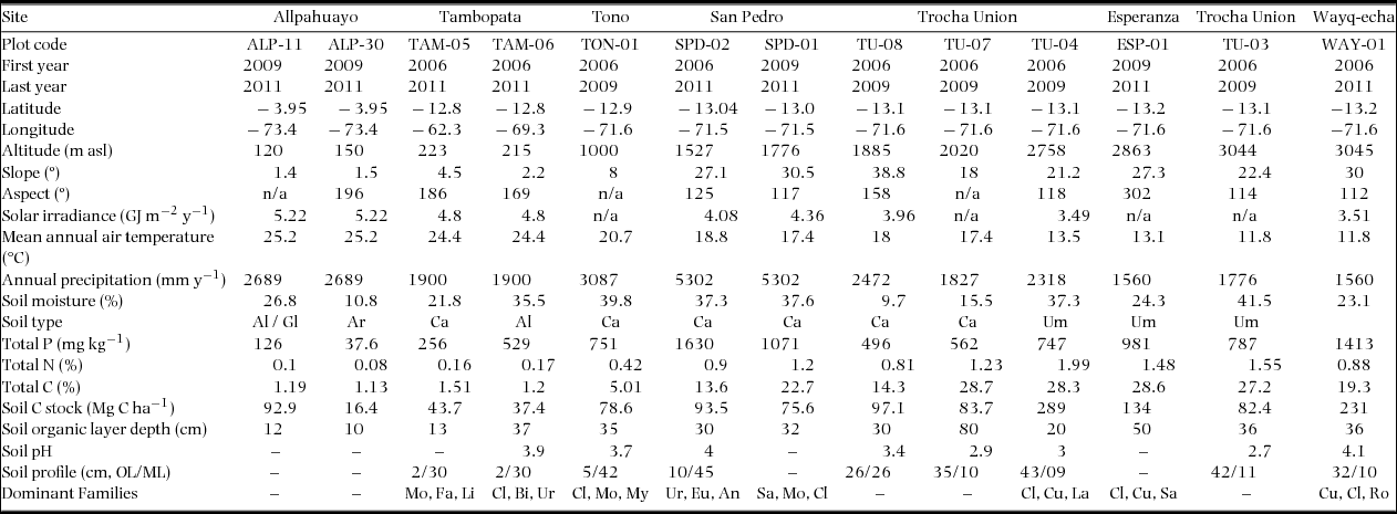
Appendix 1. Characteristics of study sites along the altitudinal gradient in the Peruvian Andes. Data from Zimmermann et al. (Reference ZIMMERMANN, MEIR, BIRD, MALHI and CCAHUANA2009), Girardin et al. (Reference GIRARDIN, MALHI, MAMANI, HUARACA HUASCO, DURAND, FEELEY, RAPP, SILVA-ESPEJO, SILMAN, SALINAS and WHITTAKER2010, Reference GIRARDIN, SILVA-ESPEJO, DOUGHTY, HUARACA-HUASCO, METCALFE, GALIANO-CABRERA, DURAND-BACA, ARAGÃO, MARTHEWS, HUARACA-QUISPE, ALZAMORA-TAYPE, EGUILUZ-MORA, FARFÁN-AMÉZQUITA, GARCÍA-CABRERA, HALLADAY, FISHER, SILMAN, MEIR, SALINAS and MALHI2014), Salinas et al. (Reference SALINAS, MALHI, MEIR, SILMAN, ROMAN CUESTA, HUAMAN, SALINAS, HUAMAN, GIBAJA, MAMANI and FARFAN2011), Huaraca Huasco et al. (Reference HUARACA HUASCO, GIRARDIN, DOUGHTY, METCALFE, DURAND, SILVA-ESPEJO, GALIANO CABRERA, ARAGÃO, ROZAS DAVILA, MARTHEWS, HUARACA-QUISPE, ALZAMORA-TAYPE, EGUILUZ-MORA, FARFAN, CABRERA, HALLADAY, SALINAS-REVILLA, SILMAN, MEIR and MALHI2014), Malhi et al. (Reference MALHI, AMEZQUITA, DOUGHTY, SILVA-ESPEJO, GIRARDIN, METCALFE, ARAGAO, HUARACA-QUISEPE, ALZAMORA-TAYPE, EGUILUZ-MORA, MARTHEWS, HALLADAY, QUESADA, ROBERTSON, FISHER, ZARAGOZA-CASTELLS, ROJAS-VILLAGRA, PELAEZ-TAPIA, SALINAS, MEIR and PHILLIPS2014), del Aguila-Pasquel et al. (Reference DEL AGUILA-PASQUEL, DOUGHTY, METCALFE, SILVA-ESPEJO, GIRARDIN, CHUNG GUTIERREZ, NAVARRO-AGUILAR, QUESADA, HIDALGO, REYNA HUAYMACARI, HALLADAY, DEL CASTILLO TORRES, PHILLIPS and MALHI2014), G. Asner and C.A. Quesada (pers comm.). Soil carbon stock was estimated from the top 0–30 cm layer. Abbreviations: nutrients: phosphorus (P), nitrogen (N), carbon (C), organic layer (OL), mineral layer (ML); soil type: Alisol (Al), Gleysol (Gl), Arenosol (Ar), Cambisol (Ca), Umbrisol (Um); dominant Families: Moraceae (Mo), Fabaceae (Fa), Linaceae (Li), Clusiaceae (Cl), Bixaceae (Bi), Urticaceae (Ur), Myristicaceae (My), Urticaceae (Ur), Euphorbiaceae (Eu), Anacardiaceae (An), Sapotaceae (Sa), Cunoniceae (Cu), Lauraceae (La), Sabiaceae (Sa), Rosaceae (Ro).


