Introduction
Large mammalian herbivores form an essential component of the natural environment in which they occur due to the impact that they have on the structure and functioning of ecosystems (Hempson et al. Reference Hempson, Archibald and Bond2015). Their preference for certain habitat types is determined by complex interactions between external factors including forage availability and quality, water availability, soil type, topography, season and predation risk (Bailey et al. Reference Bailey, Gross, Laca, Rittenhouse, Coughenour, Swift and Sims1996, O’Kane & Macdonald Reference O’Kane and Macdonald2018). Furthermore, intrinsic factors such as feeding type and morphology interact with resource competition, habitat requirements and facilitation, affecting species richness and the structure of herbivore assemblages (Cromsigt et al. Reference Cromsigt, Prins and Olff2009, Gordon & Illius Reference Gordon and Illius1996).
Herbivores select the habitat in which they feed over several temporal and spatial scales. At broader spatial extents, dispersal or migration may be necessary due to constraints of water availability, forage abundance, competition and thermoregulation, whereas at smaller extents these constraints include topography, distance from water, forage quality and quantity, and predation (Bailey et al. Reference Bailey, Gross, Laca, Rittenhouse, Coughenour, Swift and Sims1996). Along the body size spectrum, the quality of forage becomes less important than quantity of forage due to the digestive constraints of smaller herbivores (Demment & Soest Reference Demment and Soest1985). As a result, smaller herbivores exert larger search efforts compared with larger herbivores to find higher quality forage (Bailey et al. Reference Bailey, Gross, Laca, Rittenhouse, Coughenour, Swift and Sims1996). Forage quality is affected by soil nutrient content (Holland & Detling Reference Holland and Detling1990), season and regrowth as a response to herbivory and/or fire (Wilsey Reference Wilsey1996). Finally, the feeding type of herbivores is also closely related to their water dependency, with grazers and mixed feeders experiencing higher levels of water dependency than browsers (Hempson et al. Reference Hempson, Archibald and Bond2015).
The constraints under which herbivores select habitat interact with predator avoidance. In areas of diverse herbivore and predator body sizes, smaller herbivores are exposed to a greater risk of predation than larger herbivores, as both small and large predators can consume small-bodied prey (Hopcraft et al. Reference Hopcraft, Olff and Sinclair2010). Gregariousness of the species and body size affects predator-avoidance strategies, and herbivores may select more open or dense habitats dependent on the anti-predator strategies they employ (Creel et al. Reference Creel, Winnie, Maxwell, Hamlin and Creel2005, Riginos & Grace Reference Riginos and Grace2008). Herbivores are therefore regulated by top-down (predation) or bottom-up (forage quality and availability) processes (Hopcraft et al. Reference Hopcraft, Olff and Sinclair2010). These processes however may not be mutually exclusive. The underlying environmental gradients at the larger scale – soil, climate, water availability and their subsequent effect on forage quality and quantity - are therefore the primary constraints on herbivore distribution across the landscape (Bailey et al. Reference Bailey, Gross, Laca, Rittenhouse, Coughenour, Swift and Sims1996, Hopcraft et al. Reference Hopcraft, Olff and Sinclair2010).
The complexity of interactions between these processes underpins the importance of understanding savanna ecology to management. Substantial contributions to this understanding have been made by the rich history of monitoring and research which has emerged over the last century from Kruger National Park (hereafter KNP) (Biggs et al. Reference Biggs, Du Toit and Rodgers2003). KNP has a vastly heterogeneous landscape with diverse herbivore assemblages, facilitating the study of trade-offs herbivores face across multiple spatial and temporal scales. However, one of the primary environmental gradients which determines herbivore distribution, water availability, has been contentious in the context of KNP due to extensive water provision policies (Pienaar et al. Reference Pienaar, Biggs, Deacon, Gertenbach, Joubert, Nel, van Rooyen and Venter1997, Smit et al. Reference Smit, Grant and Devereux2007). In 2003, KNP had less than 8% surface area further than 5 kilometres (km) from water (Gaylard et al. Reference Gaylard, Owen-Smith, Redfern, Du Toit, Rodgers and Biggs2003). This resulted in an observable decrease in grasses and woody cover closer to artificial water points, the decline of rare herbivores due to an increase in predators, and fluctuations in common herbivore population numbers (Brits et al. Reference Brits, Rooyen and Rooyen2002, Gaylard et al. Reference Gaylard, Owen-Smith, Redfern, Du Toit, Rodgers and Biggs2003, Harrington et al. Reference Harrington, Owen-Smith, Viljoen, Biggs, Mason and Funston1999). Due to these effects, KNP management revised their water provision policy and began to close waterholes across the landscape (Pienaar et al. Reference Pienaar, Biggs, Deacon, Gertenbach, Joubert, Nel, van Rooyen and Venter1997).
Considering the increasing decline in global herbivore populations (Ripple et al. Reference Ripple, Newsome, Wolf, Dirzo, Everatt, Galetti, Hayward, Kerley, Levi, Lindsey, Macdonald, Malhi, Painter, Sandom, Terborgh and Van Valkenburgh2015, Vie et al. Reference Vie, Hilton-Taylor and Stuart2009), it is critical that a comprehensive understanding of the drivers of herbivore distribution across landscapes be developed. The study aims to test whether herbivores follow previously described trends across the Satara landscape, and to test effective means of measuring the determinants of herbivore biomass within certain habitats across a set of species which differ in functional traits. Herbivore studies typically classify species into groups of similar traits (Hempson et al. Reference Hempson, Archibald and Bond2015, Shipley Reference Shipley1999), and this provides a baseline against which to evaluate broad-level trends across different feeding types and body sizes of herbivores. Using these trends, we tested the effect of habitat attributes on 11 herbivore species at the Satara section of KNP. Herbivore studies typically look at aspects of the effects of environmental attributes on herbivores, whereas our study aims to test a combination of aspects across scales and seasons on a herbivore assemblage which differs in functional traits. We have thus tested a number of hypotheses related to the body size and feeding type of these herbivores against habitat attributes: (1) we expected risk of predation to be a stronger predictor of space use by small-bodied herbivores than larger herbivores; (2) we expected feeding type to be a strong predictor of increased daily herbivore presence in relation to distance from water because grazers tend be more water-dependent; (3) we expected the daily presence of medium-bodied grazers and small mixed-feeders to increase at higher quality forage, and large grazers increasing at higher quantity forage; and (4) we expected a strong effect of season on the biomass of grazing and mixed-feeder herbivore distribution across the landscape, with biomass and distribution decreasing further from water in the dry season and the reverse for the wet season.
Methods
Study area
This study was conducted in the Satara section (central basalt plains) of KNP, which is situated at the north-eastern corner of South Africa (24.01°S, 31.49°E). Satara receives a mean annual rainfall of 547 mm (February et al. Reference February, Higgins, Bond and Swemmer2013). The region experiences mean minimum temperatures of 10°C and 20°C and mean maximum temperatures of 26.3°C and 32.6°C in July and December respectively (Parr Reference Parr2008). The vegetation is characterized by Senegalia nigrescens/Sclerocarya birrea tree savanna (Gertenbach Reference Gertenbach1983). Habitats of this area are attractive to herbivores as two ephemeral rivers, the N’wanetsi and Sweni rivers, typically flow once or twice in the wet season and have a number of pools which may persist in the dry season. Furthermore, surface water may take longer to evaporate on the clayey basaltic soils of the region, resulting in water being more locally available across the landscape in the wet season in the form of pans (Gaylard et al. Reference Gaylard, Owen-Smith, Redfern, Du Toit, Rodgers and Biggs2003). The Letaba basalt soil type contributes to study area suitability, as it has higher calcium carbonate (CaCo3) concentrations, which gives rise to extensive grassy plains (Venter & Gertenbach Reference Venter and Gertenbach1986) that are dominated by highly palatable grass species such as Urochloa mosambicensis and Digitaria eriantha (O’Connor & Pickett, Reference O’Connor and Pickett1992). The area is also exposed to occasional wildfires and prescribed burns (Van Wilgen et al. Reference Van Wilgen, Govender, Biggs, Ntsala and Funda2004).
Site design
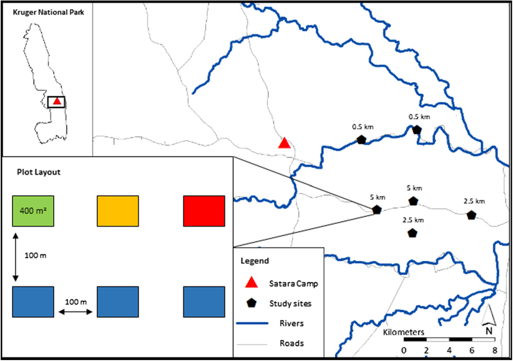
Suitable sites were identified by mapping distance to water, soil type and vegetation type as buffers of 0.5 km, 2.5 km and 5 km from all surface water (rivers and artificial waterholes), overlaid across the soil and habitat type layers using ArcGIS v10.5. (ESRI 2016). Site suitability was characterized by relative distance to water, soil type, habitat type, accessibility and the absence of previous experimental manipulation. Six sites were placed at three different distances to water, sites 0.5 km from water were situated north of the N’wanetsi river and 2.5 km and 5 km from water south of the N’wanetsi river (Figure 1). Five of the six sites fell within the Satara land type in KNP, dominated by Senegalia nigrescens/Sclerocarya birrea tree savanna, but due to constraints of site suitability one of the six sites fell within the Mavumbye habitat type, a similar land type characterized as Senegalia nigrescens bush savanna (Gertenbach Reference Gertenbach1983). Sites were sampled in June 2017, October 2017, February 2018 and June 2018, resulting in three sets of data from the late dry, early wet and late wet seasons. Wildfires occurred throughout the sampling period, resulting in one site at 2.5 km burning patchily in June 2017, and both 5 km sites burning completely in November 2017.

Figure 1. Map of the Satara section where the study was conducted, relative to the Satara Rest Camp. The site layout reads as follows: green plot = mown; yellow = mown and fertilized; red = fertilized only; blue = control. Plots were placed ∼100 m apart and were 400 m2 in size.
Each site comprised of six 20 × 20 m plots, 100 m apart, each fitted with a Cuddeback Attack Interchangeable Flash (Blue Series, Model 1255) camera trap. Plots were set up as part of a study on patch scale selection by herbivores. Camera trap data were thus the combined trapping effort of six cameras per site, each totalling an approximate area of 3.12 ha. We are confident that the plot treatments have not affected our evaluation of these landscape scale patterns, as the scale at which this paper is focused is inherently inclusive of patch scale selection in some species (Cromsigt & Olff Reference Cromsigt and Olff2006, Pretorius Reference Pretorius2009). Camera trapping is an effective, non-intrusive and replicable means of surveying mammals over a wide range of environmental and temporal scales (Carbone et al. Reference Carbone, Christie, Conforti, Coulson, Franklin, Ginsberg, Griffiths, Holden, Kawanishi and Kinnaird2001), allowing a novel means to overcome observational error of dung counts or animal observation counts.
Camera traps were fitted to each plot to have the best visual of the 400 m² plot area and were placed between 0.5 m and 1 m from the ground. They were angled away from the sun where possible, and set to a wide view angle, Fresnel cover lowered and at a wide aspect. The camera traps were set to take photographs at 10-minute intervals when activity was sensed. Finally, they were serviced (batteries replaced, and data retrieved) every 3 months, but batteries lasted on average 5 weeks, resulting in 5 weeks of data per season.
Herbivore biomass
The broad spatial and seasonal trends assessed in this study focused on water availability, forage constraints and habitat requirements of the herbivore species which commonly occur in the Satara region of KNP. These herbivore species were selected due to their representation of a suite of feeding preferences and body sizes, and the quantity of data collected by camera traps. The herbivore species were thus: five grazers (blue wildebeest Connocheates taurinus, Burchell’s zebra Equus quagga burchelli, buffalo Syncerus caffer, waterbuck Kobus ellipsiprymnus, white rhinoceros Ceratotherium simum); four browsers (common duiker Sylvicapra grimmia, giraffe Giraffa camelopardalis giraffa, greater kudu Tragelaphus strepsiceros, steenbok Raphicerus campestris); and two mixed feeders (elephant Loxodonta africana and impala Aepyceros melampus). Attributes were assigned to camera trap data as follows: date; species within the photo; number of individuals; time of day; functional characteristics (body size, feeding preference and digestive type), hereafter functional types. Feeding preference followed the three generalist functional classifications of ungulate herbivores: namely grazer, browser and mixed feeder (Gordon & Illius Reference Gordon and Illius1996, McNaughton & Georgiadis Reference McNaughton and Georgiadis1986, Owen-Smith & Novellie Reference Owen-Smith and Novellie1982). Counts data from captures were converted to the midpoint of the body weight range per species as described by Clauss et al. (Reference Clauss, Frey, Kiefer, Lechner-Doll, Loehlein, Polster, Rössner and Streich2003). As biomass values for size classes small and large were low due to low detection by camera traps, these size classes were merged with small-medium and medium-large respectively. Biomass duplications for species which remained at the site for a period of more than one hour were removed from data prior to analysis.
Environmental covariates
Distance to water was the primary determinant of site placement as it typically dictates herbivore movement (Gaylard et al. Reference Gaylard, Owen-Smith, Redfern, Du Toit, Rodgers and Biggs2003) and seasonal population fluctuations of herbivore species in savanna systems. The distances from the N’wanetsi and Sweni rivers, and the associated waterholes of the area, were used to determine suitable sites of the three distances from water. Predation was measured through camera trap data, allowing covariates of predator species, incidences of multiple predators and days since predator presence to be measured. Lion photo captures were also recorded as an individual variable due to the strong influence they have on foraging and vigilance behaviour of a range of herbivore body sizes (Périquet et al. Reference Périquet, Todd-Jones, Valeix, Stapelkamp, Elliot, Wijers, Pays, Fortin, Madzikanda, Fritz, Macdonald and Loveridge2012, Valeix et al. Reference Valeix, Loveridge, Chamaillé-Jammes, Davidson, Murindagomo, Fritz and Macdonald2009). Camera trap data were also used to determine grass height (using a marked pole in front of each camera), and plot burn data (burnt/unburnt and days since fire).
The average distance to the nearest visual obstruction was measured as a proxy for landscape of fear, given that distance to the nearest obstruction changes risk of ambush by a predator and anti-predator strategies employed by herbivore species. This value was the mean of measurements to the nearest obstruction (trees or shrubs) on each plot, using a range finder at a height of 1.5 m every 15°, totalling 24 measurements (Riginos Reference Riginos2015). The inverse of these measures was used to determine the distance between trees.
The following environmental variables were taken on each plot at each data collection period to measure forage quantity and quality: grass biomass using a disc pasture meter (Trollope & Potgieter Reference Trollope and Potgieter1986), for which the measurement value was used as a representation for biomass; grass quality using the Walker eight-point scale (Walker Reference Walker1976); and grass species were identified and a percentage cover within the plot estimated using Braun–Blanquet measure (Westhoff & Van Der Maarel Reference Westhoff, Van Der Maarel and Whittaker1978). The percentage of vigorous grass cover was determined using the mean of ‘vigorous’ values measured with the Walker eight-point scale (Walker Reference Walker1976), and used as a proxy for foliar protein using the assumption that low biomass, green grass had a higher protein content (Arsenault & Owen-Smith Reference Arsenault and Owen-Smith2008). Percentage available browse was assigned using height classes and tree counts (Riginos Reference Riginos2015). The coefficient of variation (CV) for grass biomass values was used as a measure of biomass heterogeneity, and the CV of distance to the nearest obstruction as landscape heterogeneity.
Data analysis
Camera trap data in our study had a high proportion of zeros, even when aggregated into night and day periods. We thus decided to first work on a presence/absence data to determine which environmental variables have the strongest effect on the species composition of the herbivore community. We estimated the probability of presence of a given species or functional group, using a generalized linear model for binomial data. We then investigated the drivers of biomass structure of the community by testing the variables associated with the relative biomass of the various functional groups, using presence data. We used a generalized linear model to analyse the determinants of daily observed biomass values per species and functional group biomass values for species with sufficient occurrence data for models to produce robust results. Biomass data were log-transformed to reduce large variance generated through high heterogeneity in body size, allowing data to conform to parametric analyses. All analyses were performed using R packages v3.4.1.
The dredge function in package MuMIn (Barton & Barton Reference Barton and Barton2015) was applied to the most complex models for both binomial and biomass data to generate subsets of the fixed effects of the global model. Models with AICc values which differed by <2 were then averaged using the model.avg function (Appendices A, B). Some variables retained in the average model gave estimates that had very large standard errors including 0; they were subsequently removed to simplify the final model.
Predation data were insufficient to determine an effect of predation on daily biomass. Data were initially split according to five time periods; namely pre-sunrise (00h00 to 05h59), morning (06h00 to 09h59), midday (10h00 to 13h59), afternoon (14h00 to 17h59) and night (18h00 to 23h59). In the process of determining whether predator incidence was sufficient to have an effect on herbivore presence and biomass for 24 hours thereafter (Valeix et al. Reference Valeix, Loveridge, Chamaillé-Jammes, Davidson, Murindagomo, Fritz and Macdonald2009), presence/absence and biomass values for night and day were created by merging the relevant time of day classes together. There was no significant effect of predator occurrence on any of the functional types, and we thus do not present analysis with predator incidence in the Results section, but we will briefly comment on this observation in the Discussion.
Results
Probability of occurrence
Feeding types
Binomial data models overall produced results (Table 1, Appendix C) which followed expected trends from literature. Probability of grazer presence decreased with increasing distance from water, with the effect increasing in the dry season (Figure 2a). For grazers, distance additionally interacted with grass biomass, and grazer probability of presence increased with higher grass biomass further from water (Figure 2a). We expected an increased biomass of grazers on burned sites than unburned sites, however burn effects were not selected within the ‘dredge’ process and thus did not have an effect on the overall grazer functional type.
Table 1. A summary of the expected outcomes and results produced by GLMs for binomial data for each functional type, indicating the probability of presence by a functional type at certain habitat attributes. Species traits and expectations were based on the following literature: Arsenault & Owen-Smith (Reference Arsenault and Owen-Smith2008), Clauss et al. (Reference Clauss, Frey, Kiefer, Lechner-Doll, Loehlein, Polster, Rössner and Streich2003), Gagnon & Chew (Reference Gagnon and Chew2000), Hempson et al. (Reference Hempson, Archibald and Bond2015)


Figure 2. Model simulation over the relevant gradients for the results of each feeding type’s estimated coefficients in the generalized linear model (Appendix A – Binomial values; feeding types). Values represented indicate the probability of occurrence by each feeding type predicted by the relevant environmental variables. For mixed feeders, season was not a valid descriptor of biomass; thus, values were lumped to only have three curves representing distance from water. Blue curves represent 0.5 km from water; green represents 2.5 km from water and orange represents 5 km from water.
For mixed feeders, distance did not have effects on probability of presence unless in interaction with grass biomass, and overall probability of presence was lower at higher grass biomass and at greater distance from water (Figure 2b).
Browser probability of presence increased with increasing distance from water and this effect remained consistent across seasons (Figure 2c, d). Across all distances from water, probability of browser presence was lower on burnt sites (Figure 2c). Overall, probability of browser presence was lower in the late wet season when compared with late dry and early wet seasons (Figure 2c, d).
Body size
For all body sizes, except medium-large herbivores, probability of presence was lower with increasing distance from water (Figures 3, 4). For small-medium herbivores, probability of presence increased at higher grass heights (Figure 3a).

Figure 3. Model simulation over the relevant gradients for the results of each body size’s estimated coefficients in the generalized linear model (Appendix A – Binomial values; body size classes). Values represented indicate the probability of occurrence by small-medium and medium sized herbivores predicted by the relevant environmental variables. Blue curves represent 0.5 km from water; green represents 2.5 km from water and orange represents 5 km from water.

Figure 4. Model simulation over the relevant gradients for the results of each body size’s estimated coefficients in the generalized linear model (Appendix A – Binomial values; body size classes). Values represented indicate the probability of occurrence by medium-large sized class and megaherbivores predicted by the relevant environmental variables. Blue curves represent 0.5 km from water; green represents 2.5 km from water and orange represents 5 km from water.
Medium herbivore probability of presence decreased with increasing CV (distance to nearest visual obstruction), i.e. landscape heterogeneity (Figure 3c, d). Additionally, CV and distance from water interacted, with medium herbivore probability of presence increasing at higher CV further from water. Probability of medium herbivore presence was higher on burned than unburned sites, decreasing with distance from water (Figure 3c).
Probability of medium-large herbivore presence was highest on areas of burned, short grass height, particularly in the early wet season (Figure 4a), decreasing with increased distance from water. The inverse was true for unburned areas, with medium-large herbivore presence being highest further from water (Figure 4b). Probability of presence increased with increasing distance from water in the late-dry and late-wet seasons (Figure 4a, b).
For megaherbivores, probability of presence was highest further from water and at decreased grass height (Figure 4c).
Daily biomass results
Feeding types
Daily biomass models revealed that grazer biomass decreased closer to water when grass biomass was lower and increased further from water when grass biomass was higher (Figure 5a, Appendix D). Mixed feeder biomass was highest at unburnt sites (Figure 5b). Browser biomass was overall higher further from water and increased with higher CV (distance to the nearest visual obstruction) in the early-wet and late-wet seasons (Figure 5c, d).

Figure 5. Model simulation over the relevant gradients for the results of each feeding type’s estimated coefficients in the generalized linear model (Appendix B – Biomass values; feeding types). Values represented indicate the biomass by each feeding type in relation to the functional type’s relevant describing environmental variable. Blue curves represent 0.5 km from water; green represents 2.5 km from water and orange represents 5 km from water.
Body size
Small-medium herbivore biomass was lower in the dry season than early- and late-wet seasons, was highest closer to water and increased with increasing CV (Figure 6a). Medium herbivore biomass was highest in the early wet season and highest further from water (Figure 6b). Furthermore, medium herbivore biomass increased with increasing CV at 2.5 km and 5 km from water but remained the same across all CV values at 0.5 km from water (Figure 6b).

Figure 6. Model simulation over the relevant gradients for the results of each body size’s estimated coefficients in the generalized linear model (Appendix B – Biomass values; body size classes). Values represented indicate the biomass by each body size group in relation to the functional type’s relevant describing environmental variable. Blue curves represent 0.5 km from water; green represents 2.5 km from water and orange represents 5 km from water.
Medium-large herbivore biomass was higher in the early- and late-wet seasons and closer to water on both burned and unburned sites (Figure 6c, d). Medium-large herbivore biomass decreased with increasing distance between trees at 2.5 km and 5 km from water on both burned and unburned sites, remained consistent at all distances between trees at 0.5 km on burned sites, and decreased again slightly on unburned sites at 0.5 km (Figure 6c, d).
Megaherbivore biomass was overall higher in the late-wet season than late-dry and early-wet seasons (Figure 6e).
In terms of assemblage composition, determined by habitat overlap, large changes in abundance and distribution of small mixed feeders and large grazers (Figure 7) were observed as a result of resource availability.

Figure 7. A visual representation of the assemblage composition across the three distances from water for the wet and dry season, and under two types of habitat density. Single trees on the left of each distance represent open habitat and multiple trees on the right represent dense habitat. Thickness of the line represents strength of the probability of presence by the functional types described by species of the same colour. Dark orange lines = mega-mixed feeder; light orange = small mixed feeder; black = large browser; blue = small browser; green = mega grazer; medium grey = large grazer; light grey = small-medium grazer.
Discussion
Grazers
Medium and medium-large grazing herbivores are commonly described as water-dependent, typically being found in the 0.5–2 km zone from water (Gaylard et al. Reference Gaylard, Owen-Smith, Redfern, Du Toit, Rodgers and Biggs2003). They are comparatively more dependent on surface water than browsing species, as the moisture content of grass generally falls below 10% in the dry season (Kay Reference Kay1997). Although the home range of grazing herbivores is typically closer to water during periods of drought, buffalo, waterbuck and zebra (medium-large body size class) generally occur further than 2.5 km from water (Gaylard et al. Reference Gaylard, Owen-Smith, Redfern, Du Toit, Rodgers and Biggs2003). Grazing large herbivores alter their distribution to occur further from water to mitigate poor forage conditions (i.e. forage constraints are more important than that of being close to water) (Gaylard et al. Reference Gaylard, Owen-Smith, Redfern, Du Toit, Rodgers and Biggs2003, Venter et al. Reference Venter, Prins, Mashanova, de Boer and Slotow2015). Our results show that grazers are attracted to short grass resources closer to water, whereas further from water species are attracted to high grass biomass resources which have not yet been depleted. This indicates that distance from water is a critical determinant of foraging selection patterns by species of different feeding preferences. Additionally, grass growth stage is a critical parameter of preference for a site (Murray & Brown Reference Murray and Brown1993). Accordingly, grazers will return to sites at previously grazed areas which are green with palatable regrowth (Archibald Reference Archibald2008). Our results supported this, with grazer biomass being higher at lower grass biomass at 0.5 km and 2.5 km. Furthermore, grazer biomass was highest at 2.5 km in the early wet season, following the typical magnet effect post-fire regrowth has on the distribution of grazing herbivores (Archibald et al. Reference Archibald, Bond, Stock and Fairbanks2005). Forage constraints remained the primary determinant of herbivore biomass across the landscape in the wet season, with clear preference of burnt and shorter grass areas. Finally, distance from water and grass regrowth may be a good reflection of the relationships between grazers and grass biomass, given that body size interacts with whether grazers select forage for quality or quantity, and areas of forage reserve are typically maintained further from water.
Browsers
Our models did not produce conclusive results regarding the relationship between browser biomass and the availability of browse across the landscape, and at a local scale, the relationship between browsing species and the height of browse availability described by Owen-Smith (Reference Owen-Smith1985). However, our results supported evidence that browsers are typically less water-dependent and feed >3 km from water (Gaylard et al. Reference Gaylard, Owen-Smith, Redfern, Du Toit, Rodgers and Biggs2003). It is worth noting that the browser functional type spanned across three body size classes: namely small (common duiker and steenbok), medium (kudu) and megaherbivore (giraffe), but the effect of distance from water remained consistent with browsers typically occurring further away from water. This may be more true for common duiker, steenbok and kudu, as giraffe typically feed within 0.5 km and 1 km from water (Gaylard et al. Reference Gaylard, Owen-Smith, Redfern, Du Toit, Rodgers and Biggs2003) despite being a less water-dependent species. These effects however may not be clear in our results due to the confounding nature of the body size classes within this functional type. Browsers occupy habitat further away from water due to higher moisture content of browse compared with grass (Western Reference Western1975). The relationship between browser habitat occupancy and distance to water may also be a product of the nature of the landscape. Shrub density typically increases with distance from watering points at Satara, with woody vegetation resources having been largely depleted by large herbivores as far as 2.8 km from water (Brits et al. Reference Brits, Rooyen and Rooyen2002). Giraffe and steenbok occupy mixed-habitat, and kudu and common duiker occupy closed habitat for most of the year (Pérez-Barbería et al. Reference Pérez-Barbería, Gordon and Nores2001). However, larger species are able to use a higher diversity of habitat types and are less constrained by dietary tolerance and habitat specificity than smaller species (Du Toit Reference Du Toit, Du Toit, Rodgers and Biggs2003). Our environmental covariates did not define habitats as closed-, mixed- or open-habitats, however the positive relationship between browser biomass and the distance to the nearest visual obstruction indicates that browsers we focused on prefer denser areas.
Mixed feeders
Mixed feeders are able to effectively change the utilization of grazing versus browsing resources across seasons, grazing predominantly in the wet season and browsing in the dry season. In Kruger, mixed feeders are observed to ‘switch’ from a preference of predominantly graze to browse when the 2-month concurrent mean annual rainfall has dropped below ∼30 mm (Du Toit Reference Du Toit, Du Toit, Rodgers and Biggs2003). Although it is expected that there would be a clear trend between distance to water and mixed feeder biomass, as both species are water-dependent (Redfern et al. Reference Redfern, Grant, Biggs and Getz2003), our model results did not show any clear trends, possibly due to high variation across the sample size. This could potentially be because the body size classes in this functional type spanned from small-medium (impala) to megaherbivore (elephant). Impala show preference to feeding within 1–2 km of water (Gaylard et al. Reference Gaylard, Owen-Smith, Redfern, Du Toit, Rodgers and Biggs2003) with a preference for green grass when rainfall is not limiting (Sinclair Reference Sinclair, Sinclair and Norton-Griffiths1995). Impala will revert to browsing in the dry season when green grass is not available (Du Toit Reference Du Toit, Du Toit, Rodgers and Biggs2003), as browse maintains a higher protein content for longer into the dry season than grass (McNaughton & Georgiadis Reference McNaughton and Georgiadis1986). This was supported by our results in that probability of mixed feeders was higher at shorter grass heights in the wet season when regrowth would be green. This result is likely not representative of elephant biomass, as they experience a weak relationship with forage quality, but a stronger relationship with forage quantity (Redfern et al. Reference Redfern, Grant, Biggs and Getz2003). Impala will take 2–3 day intervals between drinking although this interval can become twice as frequent in the dry season. Although elephant have shorter drinking intervals (1–2 days in the dry season) than impala, and typically feed in the riparian zone (Gaylard et al. Reference Gaylard, Owen-Smith, Redfern, Du Toit, Rodgers and Biggs2003), their feeding preference range extends as far as 3 km from water (Smit et al. Reference Smit, Grant and Devereux2007). Overall biomass trends indicate that there is an increase in mixed feeder biomass in the wet season, likely caused by higher elephant biomass in the region in the late wet season especially when elephants display increased movement across the landscape, as the constraints of forage and water availability are not as severe as in the dry season (De Knegt et al. Reference De Knegt, Van Langevelde, Skidmore, Delsink, Slotow, Henley, Bucini, De Boer, Coughenour, Grant, Heitkönig, Henley, Knox, Kohi, Mwakiwa, Page, Peel, Pretorius, Van Wieren and Prins2011).
Body size classes
Smaller herbivores have higher metabolic constraints than large herbivores due to increased energy demands (McNaughton & Georgiadis Reference McNaughton and Georgiadis1986) and their body size furthermore governs the rate and extent of energy which can be extracted from their diet. This is as a result of the retention time of food causing digestion efficiency to be lower in smaller animals than larger animals given the same food source (Demment & Soest Reference Demment and Soest1985), and thus smaller bodied species must shift to the higher protein diet provided by browse (McNaughton & Georgiadis Reference McNaughton and Georgiadis1986). Our results supported evidence that forage is the primary determinant of small-medium herbivore biomass. However, our results also indicated that smaller bodied herbivores prefer areas of increased grass height. This is in contradiction of the theory that smaller herbivores, which are more susceptible to predation (Sinclair et al. Reference Sinclair, Mduma and Brashares2003), would choose more open habitats to improve predator visibility (Riginos & Grace Reference Riginos and Grace2008). Small herbivores are usually solitary or in pairs (Hempson et al. Reference Hempson, Archibald and Bond2015), and are not able to use aggression or speed to prevent predation and thus rely on crypsis in more dense vegetation as an anti-predator strategy (Jarman Reference Jarman1974). Our models could not test against the effects of predation, and we therefore cannot speculate as to whether risk of predation would be a stronger driver of small herbivore biomass, rather than forage preference. In terms of preference for increased grass height, it is also likely that this pattern is more representative of small bodied browsers (steenbok and common duiker) (Pérez-Barbería et al. Reference Pérez-Barbería, Gordon and Nores2001), rather than the small-medium bodied impala in the wet season. This pattern will be representative of all three species in the dry season, however impala feeding preference will shift to short, green grass in the wet season as previously discussed.
For medium herbivores, the strongest predictor of biomass at a site was whether it had burnt or not, and also the homogeneity of the landscape. The medium body size class comprises wildebeest and kudu, and thus some results may be confounding. The preference for burnt areas is likely representative of wildebeest biomass, which is well documented throughout the literature (Hassan et al. Reference Hassan, Rusch, Hytteborn, Skarpe and Kikula2007, Shackleton Reference Shackleton1992, Tomor & Owen-Smith Reference Tomor and Owen-Smith2002, Wilsey Reference Wilsey1996). In times when burnt regrowth is not available, water availability may be a stronger determinant of wildebeest biomass at a site, as they typically feed in the 0.5–1 km zone, despite having longer intervals of 2–3 days between drinking. The burnt areas were at 2.5 km and 5 km from water, indicating that forage quality may be a stronger driver of wildebeest biomass than distance from water. Kudu are water-independent and typically feed >3 km from water (Gaylard et al. Reference Gaylard, Owen-Smith, Redfern, Du Toit, Rodgers and Biggs2003), and thus the relationship between decreasing medium herbivore biomass and distance from water is also more likely representative of wildebeest than kudu. Results which are not confounding however, are the relationship between distance to water and coefficient of variation on the distance to the nearest obstruction (Figure 4). Kudu are probably more representative of the 2.5 km and 5 km trend, occurring at higher biomass in denser areas (which had a higher coefficient of variation), as they are classified as species which prefer closed habitat (Pérez-Barbería et al. Reference Pérez-Barbería, Gordon and Nores2001). The function remains relatively flat for the 0.5 km zone, suggesting that homogeneity of the landscape, both in structure and composition, is not as important a driver of wildebeest biomass as forage quality and water availability.
Our results support findings that preference for burnt areas does not decrease with body size (Klop et al. Reference Klop, van Goethem and de Iongh2007, Tomor & Owen-Smith Reference Tomor and Owen-Smith2002), contrary to Wilsey (Reference Wilsey1996). Preference for burnt areas was evident in small-medium, medium and medium-large body size classes. In addition to preference of burnt areas, medium-large herbivores had a clear preference for areas of short grass (Figure 4). This is especially clear at the burnt 2.5 km zone in the early wet season, when medium-large biomass is at its highest. This further indicates that forage quality and quantity is a stronger driving factor for where medium-large biomass occurs, rather than water availability, as all the three species in this body size class (buffalo, zebra and waterbuck) typically feed in the 0.5–2 km zone from water (Gaylard et al. Reference Gaylard, Owen-Smith, Redfern, Du Toit, Rodgers and Biggs2003). Medium-large herbivore biomass is highest in the late wet season, suggesting that there are population-level movements across the park when water is less easily accessible. This is probably explained by buffalo distribution in the park across seasons, as buffalo typically move further away from water sources in the dry season to meet forage requirements of quantity rather than quality (Redfern et al. Reference Redfern, Grant, Biggs and Getz2003). This could also explain the relationship between grass height and biomass at the 5 km zone (Figure 3), although our model for binomial data does not then adequately explain the effects of season, as this trend would only make sense in the dry season. Finally, medium-large herbivores were at higher biomass with decreased distance between trees, where they might have been compelled to feed in areas of higher forage quality (Le Roux et al. Reference Le Roux, Kerley and Cromsigt2018). Forage quality is likely higher because grass layer growth may be facilitated by increased nutrient availability as a result of increased tree density (Ludwig et al. Reference Ludwig, De Kroon, Berendse and Prins2004).
Results for megaherbivores could not be clearly interpreted since the functional type comprises all three feeding preferences, namely giraffe (browser), white rhinoceros (grazer) and elephant (mixed feeder). Furthermore, elephant and white rhinoceros are classified as water-dependent species, whilst giraffe are water independent (Gaylard et al. Reference Gaylard, Owen-Smith, Redfern, Du Toit, Rodgers and Biggs2003, Hempson et al. Reference Hempson, Archibald and Bond2015), creating complex interactions with forage requirements and habitat type preference. Our model results indicated that the strongest predictor of megaherbivore biomass was the presence of short grass at 2.5 km and 5 km. This pattern could be explained by forage utilization by white rhinoceros, as they prefer feeding on short grass areas (McNaughton & Georgiadis Reference McNaughton and Georgiadis1986, Pretorius Reference Pretorius2009, Waldram et al. Reference Waldram, Bond and Stock2008). The relationship between grass height and distance from water at 0.5 km indicates that grass height was not a valid predictor of megaherbivore biomass close to water, where giraffe are most likely to feed (Gaylard et al. Reference Gaylard, Owen-Smith, Redfern, Du Toit, Rodgers and Biggs2003).
Finally, assemblage composition differed across season as a result of altered forage use by the small-mixed feeder and large grazer functional types. In the wet season when resource quality is improved and water is more uniformly distributed across the landscape (Gaylard et al. Reference Gaylard, Owen-Smith, Redfern, Du Toit, Rodgers and Biggs2003), the abundance of grazers and mixed feeders increases. Furthermore, the change in resource quality causes small mixed feeders and large grazers to alter their resource use from browse and tall grass swards respectively, to short grass swards which contain less fibre and increased crude protein (Arsenault & Owen-Smith Reference Arsenault and Owen-Smith2008, Du Toit Reference Du Toit, Du Toit, Rodgers and Biggs2003, Kutilek Reference Kutilek1979). In the wet season, assemblages close to water comprise largely grazers across the body size spectrum, particularly in more open, short grass habitats, mixed feeders across the body size spectrum, with few large browsers. Further from water, assemblages comprise fewer grazers and more browsers across the body size spectrum, particularly in denser habitat of increased grass height. In the dry season, assemblages close to water comprise largely of medium grazers, which occupy open habitat of short grass height, and mega-mixed feeders. As the distance from water increases, assemblage composition includes more small mixed feeders, browsers and large grazers, particularly in denser habitat of increased grass height. Furthest from water, assemblages comprise largely of large grazers and browsers, particularly in denser habitat of increased grass height, megagrazers at short grass height, and mega-mixed feeders.
Conclusion
Our results supported trends across body size classes and feeding types which have previously been described. However, herbivore studies have typically looked at aspects of the effects of environmental attributes on herbivores, whereas our study has tested a combination of aspects across scales and seasons, on a herbivore assemblage which differs in functional traits. The results of this study showed that water availability and forage quality and quantity largely alter the composition of the assemblage, particularly in the grazer and mixed feeder guild. The means utilized to test predation effects were insufficient to explore the relationship across functional types, indicating that broad-scale camera trap surveys, in our case, may not have been an effective tool in this regard.
The use of distance from water and grass regrowth measurements to reflect grazer biomass warrants more investigation at a less coarse grain, especially in areas further from water and which experience less grazing pressure. Finally, the models developed in this study are a comprehensive analysis of a wide spectrum of body sizes and feeding types across a broad environmental gradient. The detection and confirmation of previously described trends indicates that the use of environmental attributes in GLMs may be a useful means to predict herbivore presence across seasons at a landscape scale.
Acknowledgements
We thank South African National Parks and the Scientific Services division of Kruger National Park for their permission to work in KNP. Furthermore, the game guards and technicians who assisted in the development and servicing of the sites over the course of the year, in particular Happy Mangena. Thank you to Christopher Brooke for assistance with graphics, Yentl Swartz and Zanri Schoeman for the use of silhouette images in this paper. Nelson Mandela University, Fairfield Tours and DST-NRF grant 112199 supported C. Young’s research.
Appendix A
AICc value comparisons for global and final generalized linear models by functional types by binomial data. Final models are the product of the global model with the lowest AICc value, following the removal of variables which had large standard errors including 0.

Appendix B
AICc value comparisons for global and final generalized linear models by functional types for biomass data. Final models are the product of the global model with the lowest AICc value, following the removal of variables which had large standard errors including 0.

Appendix C
Results from the final generalized linear model selected for each functional type – binomial data.

Appendix D
Results from the final generalized linear mixed model for each functional type – Biomass data.