INTRODUCTION
Animals are often present in locations that match species-specific preferences and physical tolerances, in accordance with the need to acquire food, reproduce and defend themselves (Hamilton Reference HAMILTON1971). When these biological or physical needs are not met, many organisms make large or small-scale vertical or horizontal movements in order to increase their chance of survival. In addition, over geological timescales, species evolve to effectively utilize their habitat to increase their fitness. For example, there are four marine lakes in the small island nation of Palau each having a different subspecies of golden jellyfish (Mastigias papua) that has its own separate genetic, physical and behavioural characteristics (Dawson Reference DAWSON2005, Hamner & Hauri Reference HAMNER and HAURI1981, Hamner et al. Reference HAMNER, GILMER and HAMNER1982). In particular, in Jellyfish Lake, Mastigias papua etpisoni has adapted and evolved unusual behavioural strategies and sensory responses to environmental conditions over the last 10 000 y (Hamner et al. Reference HAMNER, GILMER and HAMNER1982). It is currently unknown what conditions maximize their survival, largely because it is a challenge to collect data on both the individual organism and the environment on a scale that matters to individuals.
Millions of Mastigias papua etpisoni are nearly always present in Jellyfish Lake but their population can be sensitive to environmental shifts. For example, during 1997–1998, the medusae population disappeared from the lake, associated with high water temperatures related to the El Niño Southern Oscillation (Dawson et al. Reference DAWSON, MARTIN and PENLAND2001, Martin et al. Reference MARTIN, DAWSON, BELL and COLIN2006) but the benthic jellyfish polyps in the lake survived and the medusae population eventually recovered in 2000 as temperatures cooled. The recovery of this jellyfish population is important to Palau's economy because Jellyfish Lake has become one of the most popular tourist snorkelling destinations. Therefore, assessing the distribution and abundance of the Mastigias papua etpisoni population in relation to its lifecycle and habitat features is therefore economically significant and ecologically important for understanding its biophysical connection to oscillating climate dynamics.
A general understanding of Mastigias papua etpisoni population, lifecycle and movements are known. The population of Mastigias papua etpisoni normally consists of the full size spectrum due to continuous reproduction (Hamner & Hauri Reference HAMNER and HAURI1981, Hamner et al. Reference HAMNER, GILMER and HAMNER1982). Mastigias papua etpisoni largely relies on the photosymbiotic zooxanthellae within its tissues for its food needs, but also acquires energy and nutrients through stinging cell capture of zooplankton, principally copepods. Because sunlight is needed to sustain zooxanthellae, Mastigias papua etpisoni makes a daily west-to-east migration across the lake. This 1-km-long migration ensures Mastigias papua etpisoni individuals receive adequate sunlight for photosynthesis, but also stay out of shadows cast by vegetation and high hills on the lake's edge, decreasing encounter rates with the predatory sea anemone (Entacmaea medusivora) residing at the lakeside (Dawson & Hamner Reference DAWSON and HAMNER2003). Through this daily routine, Mastigias papua etpisoni maximizes photosynthetic rates and minimizes predation.
In this study, we aim to demonstrate a non-invasive, highly efficient and novel approach to map Mastigias papua etpisoni abundance and distribution in relation to environmental properties in this protected marine lake. We hypothesize that the jellyfish population will mainly be present on the eastern side of the lake during our midday surveys. We expect the distribution of jellyfish throughout the lake to be patchy with discrete patches of higher densities of jellyfish, which would suggest individuals have varying responses to biological or physical cues that initiate or halt their migration, or individuals migrate at different rates. We also hypothesize that the vertical distribution of jellyfish will be related to water column properties and match physiological tolerances. We anticipate that occupying a specific depth range provides jellyfish with adequate oxygen for respiration and light for photosynthesis.
METHODS
Study site and species
In the Western Pacific, Jellyfish Lake (locally known as Ongeim'l Tketau) is located on Mecherchar Island in the Rock Islands Southern Lagoon, Palau (07 09.83′N, 134 22.50′E; Figure 1), and is inhabited by perennial jellyfish blooms. It is an isolated marine lake that is indirectly connected to the ocean through cracks, fissures and tunnels in limestone. The lake is brackish and stratified by an excess of precipitation over evaporation and has limited wind and tidal-driven mixing (Hamner & Hamner Reference HAMNER and HAMNER1998, Hamner et al. Reference HAMNER, GILMER and HAMNER1982). The tides in Jellyfish Lake are damped 25% of the lagoon tide with a 2.5-h time lag (Hamner & Hamner Reference HAMNER and HAMNER1998). For the protection of Mastigias papua etpisoni, motorized boats are prohibited in the lake and all instrumentation has to be carried in and out overland. All research conducted was approved by the Bureau of Marine Resources and the Koror State Government.
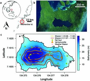
Figure 1. The Republic of Palau is a small island in the western Pacific (a), Jellyfish Lake is located in Mecherchar (photo credit: P. Colin) (b), the REMUS autonomous underwater vehicle was deployed within Jellyfish Lake, and ran two nearly identical missions on the morning of 24 March 2011 (local time) (c). * represent locations of underwater limestone tunnels from Hamner & Hamner (Reference HAMNER and HAMNER1998).
Jellyfish Lake is principally inhabited by Mastigias papua etpisoni. Mastigias papua etpisoni individuals are known to migrate at sunrise towards the east from all areas of the lake and return west following the sun in the afternoon (Hamner & Hauri Reference HAMNER and HAURI1981). After sunset, individuals make repeated vertical migrations throughout the oxygenated layer from the surface to the chemocline in order to uptake nitrogen needed by zooxanthellae for photosynthesis (Hamner et al. Reference HAMNER, GILMER and HAMNER1982, Muscatine & Marian Reference MUSCATINE and MARIAN1982).
Vertical profiles and net sampling
We measured the water properties and abundance of Mastigias papua etpisoni in Jellyfish Lake. On 16 March 2011, measurements of vertical water column properties were made on the west and east side of the lake between 9h51–10h10 and 10h34–10h46 (local time, Figure 1c). From a Caddisfly floating chair, data were collected at 1 m intervals from 0–24 m using a Hydrolab DS5 Water Quality Sonde with the following sensors: temperature, conductivity, pH, chlorophyll-a (CHL), Hach LDO dissolved oxygen, and Li-Cor Ambient Light (or Photosynthetically Active Radiation (PAR) sensor) (OTT Hydrometry Ltd). Past studies have shown the upper oxygenated mixed layer is separated from a deeper anoxic layer by a floating bacterial plate dominated by purple photosynthetic, sulphur bacteria (Chromatium sp.) at ~15 m (Hamner et al. Reference HAMNER, GILMER and HAMNER1982). The depth and thickness of the bacterial plate was studied from water samples collected by means of a Nansen bottle. Water samples collected at 0.5-m intervals were tested for smell and colour. The bacterial plate was identified by a pink colour and the smell of hydrogen sulphide. We tested for differences in the physical parameters on the west and east side of the lake and tested for correlations between parameters using a Pearson's correlation.
On 17 March 2011, three replicates of a set of 15 evenly spaced vertical net hauls (Figure 1c; net radius (r) = 0.25 m, 1-mm mesh) were taken from 15 m depth to the surface, which is standard protocol for monthly observations (Martin et al. Reference MARTIN, DAWSON, BELL and COLIN2006). The three surveys began at 9h40, 11h15 and 13h10, and lasted ~40 min each. Temporal spacing of the surveys allowed sampling during different phases of the well-documented jellyfish migration in this lake (Dawson & Hamner Reference DAWSON and HAMNER2003, Hamner & Hauri Reference HAMNER and HAURI1981). The only species caught in the nets was Mastigias papua etpisoni. During each survey, all jellyfish were placed into bins, and were counted and measured after all of 15 vertical tows were completed allowing for more rapid sampling of the lake. Bell diameter (BD) of each medusa was measured in 0.5 cm increments. The number of medusae was summed for the 15 net hauls within each replicate, and Mastigias papua etpisoni abundance was estimated three times using this number of jellyfish (J) and the area of the lake (A = 61 000 m2),
 $$\begin{equation*}
{\rm{Jellyfis}}{{\rm{h}}_{{{Abundance}}}} = A\frac{J}{{15{r^2}\pi }}
\end{equation*}$$
$$\begin{equation*}
{\rm{Jellyfis}}{{\rm{h}}_{{{Abundance}}}} = A\frac{J}{{15{r^2}\pi }}
\end{equation*}$$
From the three replicates, an average population estimate and standard deviation for the day was determined. We also determined jellyfish abundances in 1-cm size class increments from 0–15 cm for comparison with acoustic estimates.
A floating weather station on a 3 m tripod was located midway between the east and west basin of the lake (07 9.67′N, 134 22.61′E). It had a rain gauge (Texas Electronics TE525-WS) and marine model wind speed and direction sensor (RM Young 05106 Wind Monitor-MA) and provided hourly weather measurements. This information was included because large storms and thus, vertical mixing, could affect the distribution and abundance of jellyfish.
REMUS autonomous underwater vehicle
Acoustic techniques are commonly used to estimate the distribution and abundance of fishes and zooplankton over large areas because these surveys can be conducted relatively quickly. Acoustic methods are usually paired with short-term optics or capture of species for size frequency and abundance validation. These types of traditional sampling methods (i.e. net tows) are useful for providing morphological and taxonomic information but are often problematic for jellyfish, which have fragile tissues that can be minced, or large aggregations can clog or destroy nets (Brierley et al. Reference BRIERLEY, AXELSEN, BUECHER, SPARKS, BOYER and GIBBONS2001). In addition, these methods often provide only semi-quantitative estimates of abundance (Brodeur et al. Reference BRODEUR, MILLS, OVERLAND, WALTERS and SCHUMACHER1999, Purcell Reference PURCELL2003) because medusae patchiness cannot be resolved (Graham et al. Reference GRAHAM, PAGÈS and HAMNER2001). Echosounders have been integrated into autonomous underwater vehicles (AUVs) that are also equipped with other sensors to simultaneously measure the biological and physical environment (Benoit-Bird et al. Reference BENOIT-BIRD, MOLINE and SOUTHALL2017), but not yet attempted for the study of jellyfish.
We used a propeller-driven REMUS-100 AUV (augmented with a propeller guard) to map the distribution and abundance of Mastigias papua etpisoni and record measurements of the physical environment of Jellyfish Lake. The REMUS is torpedo-shaped, has a length of 160 cm, a diameter of 19 cm, a depth range of 0 to 100 m, weighs 37 kg, and with two people can be hand deployed (Moline et al. Reference MOLINE, BLACKWELL, VON ALT, ALLEN, AUSTIN, CASE, FORRESTER, GOLDSBOROUGH, PURCELL and STOKEY2005). The REMUS uses a compass for heading, Doppler Velocity Log (DVL) for speed and altitude over the bottom, pressure sensor for depth, GPS for surface navigation, and acoustic transponders for precise underwater navigation (Moline et al. Reference MOLINE, BLACKWELL, VON ALT, ALLEN, AUSTIN, CASE, FORRESTER, GOLDSBOROUGH, PURCELL and STOKEY2005). The REMUS was equipped with sensors to measure temperature, salinity, bathymetry and acoustic backscatter. The REMUS had a YSI CTD that sampled at a 4-s interval. A single-beam 217 kHz BioSonics DT-X portable digital scientific echosounder was integrated into the REMUS vehicle and oriented to look upwards while the vehicle swam at depth. The echoes were not corrected for their position in the beam because this is a single-beam system. The system was calibrated by BioSonics Inc. using a reference-standard transducer in their hydroacoustic calibration facility. The echosounder had a beam width of 5.7°, a transmit source level of 221.9 dB µPa−1 and receiver sensitivity of –51.5 dB µPa−1. The minimum data collection threshold was set to −150 dB. Data were collected within a range of 0–15 m from the echosounder transducer. The transducer had a ping rate of 5 pings s−1, and a transmit pulse duration of 0.1 ms. A GoPro Hero 2 camera was also mounted on the REMUS facing upwards and recorded video. This allowed for visual identification of Mastigias papua etpisoni, but due to the turbidity of the water these images were not clear enough for any quantitative abundance estimates (Figure 2a, b).

Figure 2. Photographs showing jellyfish (Mastigias papua etpisoni) swarms in Jellyfish Lake, Palau. Jellyfish viewed from ~8 m depth (a), jellyfish near the lake's surface (b), both photos were taken using a GoPro attached to the REMUS. Note the high variation in jellyfish body orientation. An aerial view of the jellyfish aggregation in the south-east corner of the lake in January 2008 (photo credit: P. Colin) (c). Note the shadow cast on the lake by the trees.
On 24 March 2011, the REMUS ran two missions beginning at 10h38 and 11h07, lasting 24 and 23 min and travelled a distance of 1911 m and 1833 m at an average speed of 1.3 m s−1. We aimed mission times to coincide with the times of minimal jellyfish movement and overlap with the timing of net tows and vertical water column profiles. While the REMUS surveys occurred 1 wk after net surveys, we expect no major differences in jellyfish size and abundance as the medusa grow only ~1 cm wk−1. The REMUS maintained a depth of ~8 m, as visual observations and past studies (Dawson & Hamner Reference DAWSON and HAMNER2003, Hamner et al. Reference HAMNER, GILMER and HAMNER1982) throughout the lake revealed few, if any, jellyfish are below this depth during the day. This depth minimized potential disturbance and maintaining a shallower depth (than vertical net tows) allowed us to survey closer to the shallow lakesides and avoid the bacterial plate. The difference between the REMUS track in mission 1 and mission 2 (Figure 1c) was the result of acoustical navigation challenges, where sound likely reflected in unpredictable ways off steep walls within the confined space of the lake.
The acoustic backscatter data were processed in BioSonics’ Visual Acquisition 6 and Visual Analyzer 4.3 software. We limited our analysis from the surface to 0.5 m from the vehicle to remove sound intensity distortions due to the transducer near field or any near-vehicle effects. Using Visual Analyzer, identification of the lake surface was done manually. Average temperature and salinity recorded on the vehicle's CTD was used to calculate sound speed and absorption coefficients. In Visual Analyzer, the mean backscattering cross section and target strength (TS) for jellyfish was estimated using the Expectation Maximization and Smoothing (EMS) method (Hedgepeth Reference HEDGEPETH1994, Hedgepeth et al. Reference HEDGEPETH, GALLUCCI, O'SULLIVAN and THORNE1999), which is a robust iterative statistical technique that is useful for single-beam data. A minimum of 200 targets were required for completion of the EMS procedure. This EMS technique is based on the distribution of targets versus TS and the probability of placement within the acoustic beam. The number of acoustic targets was estimated using echo integration, which allows the measured energy return for a given volume of water to be used to estimate target populations. Visual Analyzer's echo integration method uses the above TS estimation technique to obtain a mean backscattering cross-section value so that the density of jellyfish can be estimated. For analysis, the TS range was set to −65 to −85 dB, which removed all background noise and other very weak unwanted echoes. Other echo recognition parameters included a correlation factor of 0.9, minimum and maximum pulse width factor of 0.2 and 3, and end point criteria of −6 dB. The measurements were binned into 1 m bins from the vehicle to the surface and into 7 m bins along the vehicle track. The acoustic surveys provided areal (jellyfish m−2 in the sampled water column) and volumetric (jellyfish m−3) estimates of jellyfish density. The accurate conversion from echo integration to animal densities depends on estimates of individual TS (Simmonds & MacLennan Reference SIMMONDS and MACLENNAN2005). However, because no laboratory tests were conducted to identify the TS range for Mastigias papua etpisoni, we ran a sensitivity analysis to determine how changing the lower echo threshold altered the number of jellyfish detected. For rapid processing, we ran the above echo integration procedure on a subset of data and changed the minimum echo threshold from −65 dB to −90 dB in 1 dB increments for each iteration. The results from this test combined with visual observation of the echograms confirmed a threshold of −85 dB was appropriate for our dataset (Appendix 1). We excluded all targets that were unlikely to be jellyfish, based on the size, shape and level of the acoustic return. For example, high acoustic returns on the surface could be floating debris (i.e. fallen logs, leaves, sticks), snorkellers, or bubbles generated from human action. Jellyfish Lake is a major tourist attraction where people can freely snorkel. Other species that inhabit the lake that could produce acoustic backscatter include copepods (Oithona and Acrocalanus), and silverside fish (Pranesus) (Hamner & Hamner Reference HAMNER and HAMNER1998). However, copepods are likely too small to be detected at 217 kHz except at high densities.
Spatial analysis
Kriging was used to estimate the spatial distribution of jellyfish between REMUS survey lines. Kriging is a well-established geostatistical technique for spatial interpolation that allows values to be obtained at points without direct observations from neighbouring areas using spatial autocovariance (Cressie Reference CRESSIE1988, Journel & Huijbregts Reference JOURNEL and HUIJBREGTS1978). Ordinary kriging was performed using the package ‘geoR’ in R (Ribeiro & Diggle Reference RIBEIRO and DIGGLE2001). This was also done for temperature, salinity and density but first, we omitted all observations at depths that outside of the 15–85% depth quantile to reduce any error associated with slight differences in vehicle depth. Rigorous care was taken to ascertain the depth of the vehicle was not driving spatial variation in water properties. All grids were converted to the same extent with 5 × 5-m grid cells. An example of jellyfish density along the REMUS track, kriged values and variance is shown in Appendix 2. Jellyfish abundance estimates were calculated by multiplying jellyfish density by the area of the grid cell and summing across the grid. To investigate the spatial distribution of jellyfish by longitude, we grouped jellyfish density into 44 bins with 0.0001 degrees longitude spacing (for each bin n > 85). We also visualized the vertical distribution of jellyfish density in 1-m bins from 0–9 m (n > 200). We tested for significant differences in jellyfish density between mission 1 and mission 2 for each depth bin using a t-test. We also tested for significant differences between all depth bins using a non-parametric Kruskal–Wallis test and a multiple comparison test after Kruskal–Wallis for each respective mission.
RESULTS
During our study period of 16–24 March 2011, in Jellyfish Lake the weather was mild, with total rainfall of 52.6 mm, an average wind speed of 1.2 ± 0.8 m s−1, and most frequent wind direction was from the north-north-west. On 16–17 March 2011, physical and biological parameters were measured as a function of depth on the west and east side of Jellyfish Lake (Figure 3). On 16 March when water properties were measured, there was a total of 1.8 mm of rain, average wind speeds of 0.9 ± 0.6 m s−1 from the west-south-west and on 17 March when jellyfish net hauls were done, there was a total of 12.7 mm of rain, average wind speeds of 1.0 ± 0.5 m s−1 from the south-south-west. This suggests there were no significant weather events to alter the behaviour of Mastigias papua etpisoni during these survey days.
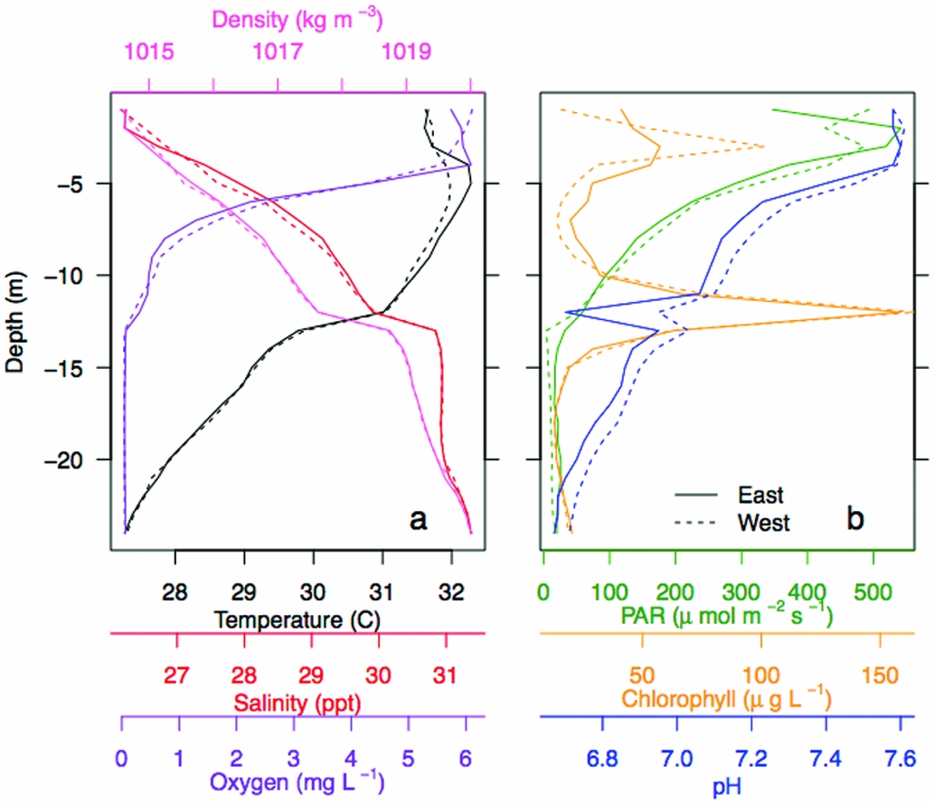
Figure 3. Vertical water column structure of Jellyfish Lake, Palau. Vertical profiles of water temperature, salinity, oxygen and water density (a), and photosynthetic active radiation (PAR), chlorophyll-a concentrations, and pH at the east and west survey site (b).
Vertical properties of the water column showed oxygen was high (~5.5–6 mg L−1) in the upper 4 m and decreased with depth to anoxic levels below 13 m (~0 mg L−1, Figure 3a). Surface water temperature (< 2 m) was cooler (~31°C), with a slight increase (~32°C) from 5–7 m. Temperature linearly decreased below 10 m to a minimum of 27.3°C. Salinity steadily increased from 26 to 31.4 ppt from the surface to 24 m. pH was ~7.6 at the surface, decreased steadily below 4 m and was the lowest at ~6.7 at 24 m (Figure 3b). PAR was high (800–1200 umol m−2 s−1) at the surface, decreased with depth and was < 60 µmol m−2 s−1 below 12 m. Chl concentrations peaked at ~75 and 150 µg L−1 at ~3 m and 12 m. Water density increased with depth from ~1015 to ~1020 kg m−3, with the pycnocline at 13 m. Vertical profiles for each parameter were similar on the west and east side of the lake (Pearson correlation, r > 0.94). There was a strong negative correlation with salinity and the following variables: pH, oxygen, PAR and temperature on the west and east side (r < −0.80; Appendix 3). There was a strong positive correlation between pH, temperature, PAR and oxygen (r > 0.50; Appendix 3). CHL was not strongly related to any of these variables (r < 0.40). Separating the upper oxygenated mixed layer from the deeper anoxic layer was a floating bacterial plate that was seen in peak CHL at 12 m (Figure 3). Water samples of the plate showed that it was thin, ~0.25 m. A change in physical variables was apparent above and below this layer, maintained by a strong density gradient, with modifications in salinity, temperature, light and oxygen below the bacterial plate.
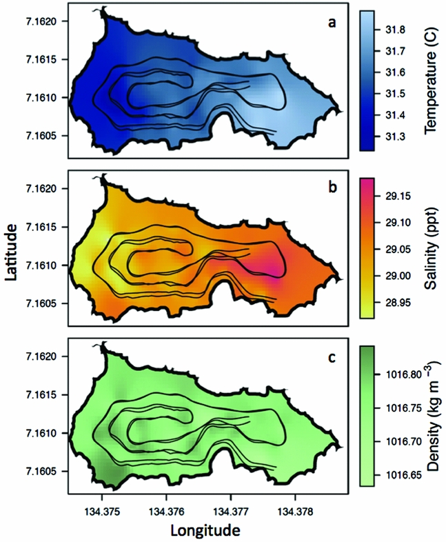
On 24 March 2011, the REMUS ran two nearly identical missions lasting ~25 min each (Figure 1c). On this day, the weather was mild with no rain and average wind speeds of 1.6 ± 0.9 m s−1 from the north. On average, at ~8 m depth, the temperature of the lake was 31.6 ± 0.1°C, the salinity was 29.0 ± 0.05 ppt and the density was 1016.8 ± 0.02 kg m−3 (Figure 4). At ~8 m, the west side of the lake was cooler by ~0.5°C, had a lower salinity by ~0.3 ppt but a slightly higher density by ~0.2 kg m−3 whereas the east side was warmer, saltier and less dense (Figure 4), mirroring vertical profile measurements from 16 March 2011 (Figure 3). The agreement between vertical profiles and horizontal REMUS surveys on the west and east side of the lake support that any depth variations of the REMUS that were not accounted for did not hinder our ability to detect changes in physical properties from west to east and reveals how widespread this gradient was.

Figure 4. Spatial variability of water properties in Jellyfish Lake, Palau. Water temperature (a), water salinity (b) and water density (c) measured from the REMUS at ~8 m depth. The REMUS tracks are plotted for reference.
Using the REMUS, we acoustically mapped the distribution and abundance of Mastigias papua etpisoni for the first time. Echograms clearly showed discrete acoustic returns from individual jellyfish as confirmed with video recordings (Figure 5). The echograms also revealed some unidentified clusters at the surface, probably debris from trees or people snorkelling, and occasionally unknown scatters at depth, perhaps schools of small fish (Figure 5). Our echo integration threshold test confirmed our procedure was adequate, where similar estimates of jellyfish abundance and density were attained using an echo threshold of −84 to −88 dB (Appendix 1). The average TS of individual jellyfish was −81.0 ± 3.03 (n = 48 375) at 217 kHz (Table 1) and the distribution of TS showed most jellyfish had TS between −79 to −85 dB (Figure 6a). On 17 March 2011, the average jellyfish BD from net sampling was 3.40 ± 4.43 cm, ranging from 0.5 to 15.5 cm (Figure 6b). There was a bimodal distribution of jellyfish size classes with very few jellyfish with BDs between 3–6 cm and ~63% of medusae BDs, from all net hauls, were ≤ 0.5 cm (Figure 6b).

Figure 5. An example of a volume backscattering (Sv) echogram at 200 kHz from 11h19–11h21 in Jellyfish Lake, Palau. Acoustic scattering was plotting with a 40logR time varying gain correction, which is appropriate for single targets. The REMUS was at a depth of ~8 m with the echosounder transducer facing upward towards the lake's surface. Jellyfish (Mastigias papua etpisoni) can be seen throughout the echogram. Two unknown high acoustic return clusters could result from debris on the surface or a fish school at depth; these types of rare, yet unidentified clusters were removed from the data analysis.
Table 1. Comparison of jellyfish bell diameter (BD) and acoustic target strength (TS) of different jellyfish species using a 200-kHz echosounder. The mean ± SD or range in BD and TS is summarized.


Figure 6. Distribution of jellyfish (Mastigias papua etpisoni) target strength and bell size in Jellyfish Lake, Palau. The number of jellyfish detected by target strength in 2 dB bins (a). The size frequency distribution in per cent (n = 1023) of medusa bell diameter in March 2011 (b).
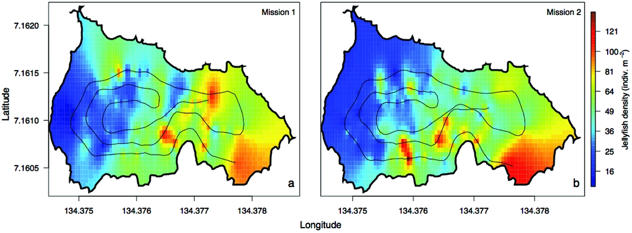
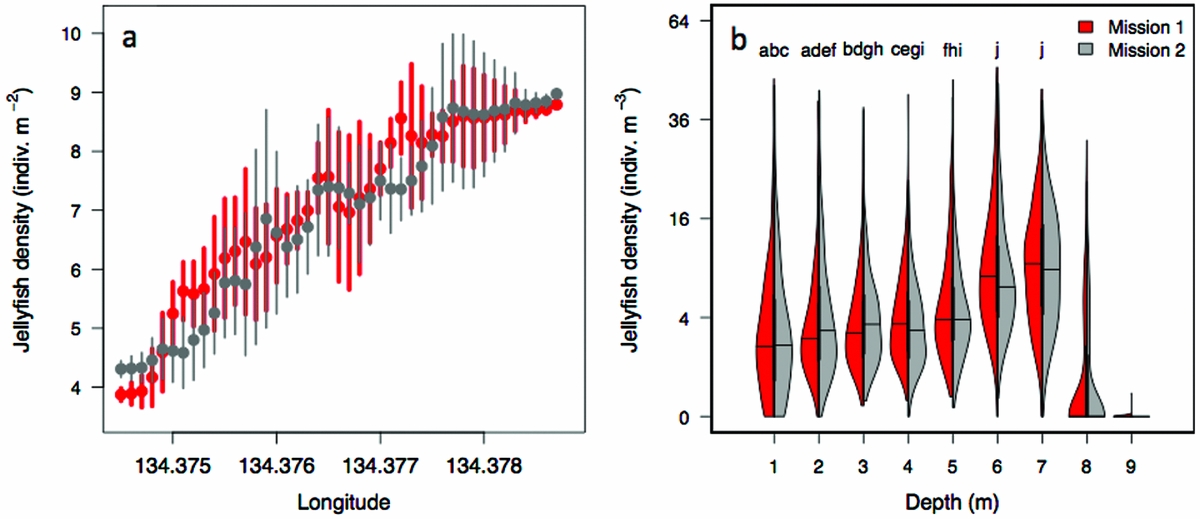
The density of Mastigias papua etpisoni measured by the REMUS, varied spatially and vertically. Spatially, the density of Mastigias papua etpisoni as estimated from REMUS surveys, increased linearly across the lake from the west to east from an average of ~4–9 jellyfish m−2 (Figure 7, Figure 8a), but the distribution of jellyfish was patchy during both missions with a few areas having dense aggregations of more than 120 jellyfish m−2 (Figure 7). While the two REMUS missions were only 30 min apart and showed very similar results, the eastward migration of jellyfish was apparent between mission 1 and mission 2 (Figure 7). Visualizing each mission separately also revealed the jellyfish patchiness, which may have been obscured if the missions were averaged together. These patterns in jellyfish density mirror volume backscattering (Sv) measured along the vehicle's track (Appendix 4). Extrapolated density estimates outside of the vehicle's track should be regarded as tentative as these were not direct measures, especially densities within the south-east corner of the lake where the kriging variance was higher (Figure 7, Appendix 2). However, comparison of an aerial image (Figure 2c) with density estimates (Figure 7) revealed a similar jellyfish distribution and demonstrate that the south-east corner does indeed have a higher abundance of jellyfish during midday. The aerial image was taken at a different date, but it should be noted that jellyfish daytime distribution patterns are very consistent. Vertically, the density of Mastigias papua etpisoni ranged from 0–~60 jellyfish m−3 (Figure 8b) between the surface and 9 m depth with no significant differences in density at each depth between mission 1 and mission 2 (t-test, P > 0.05). Mastigias papua etpisoni density was often significantly different between distant depth bins (multiple comparisons test after Kruskal–Wallis, P < 0.05; Figure 8b). Generally, Mastigias papua etpisoni density was not significantly different between 1 to 5 m; highest densities were between 6–7 m (not significantly different from each other, P > 0.05) with lowest densities below 7 m and virtually no jellyfish at 9 m. While vertical net hauls ranged from 0–15 m and REMUS estimates were between ~0–8 m, these findings (Figure 8b) coupled with visual observations from swimmers and past studies revealed no jellyfish were below 9 m making net hauls and REMUS survey data comparable. From the three sets of net hauls, the mean density of jellyfish was 115.78 ± 22.84 m−2.

Figure 7. Spatial distribution of jellyfish (Mastigias papua etpisoni) density during mission 1 (a) and mission 2 (b) in Jellyfish Lake, Palau. The REMUS track is plotted for reference.

Figure 8. Horizontal and vertical distribution of jellyfish (Mastigias papua etpisoni) during mission 1 and mission 2 in Jellyfish Lake, Palau. The mean and SD in jellyfish density by longitude (a). Probability density of jellyfish density by depth (b). Data was grouped into 1-m depth bins. Individual letters indicate non-significant differences in the mean between depth bins for both missions with the exception of f, which was only non-significant in mission 2. Thick black lines specify the interquartile range, thinner black lines are the upper and lower adjacent values, and horizontal lines are the median.
Jellyfish abundance estimates were made from both acoustic data and net hauls. From acoustic surveys, the estimated abundance of Mastigias papua etpisoni was 2.8 and 2.7 million for mission 1 and mission 2. From net samples, the abundance estimate for all size classes was 7.1 ± 1.4 million jellyfish. When jellyfish below 1 cm BD were excluded, the abundance estimate was 2.6 ± 0.5 million jellyfish (Figure 9), and abundances estimates were similar for BDs ≥3, ≥4, ≥5, ≥6 and ≥7 cm, roughly 2.0 million (Figure 9).

Figure 9. Jellyfish (Mastigias papua etpisoni) abundance estimates (mean ± SD) in Jellyfish Lake, Palau, from net hauls by bell diameters in 1 cm increments, excluding smaller size classes below each threshold. Jellyfish abundance estimate from acoustics data is shown by the black dashed line.
DISCUSSION
Understanding species-habitat relationships require measurements of both the species’ distribution and the habitat occupied on a similar spatiotemporal scale. While AUVs can require substantial effort for mission planning and sensor integration, the quality and quantity of data from AUVs demonstrate Mastigias papua etpisoni distribution, abundance and habitat can be simultaneously measured in less than 1-h. Comparable data from net samples and vertical profiles required about 5 h to collect, indicating the relative efficiency and utility of the AUV. An AUV is the most suitable tool for measuring abundance, given that all motorized boats are prohibited in the lake and any surface platform (i.e. kayak or rowing boat towing an echosounder at depth) would disturb the jellyfish that are highly abundant at the surface. As the acoustic targets in Jellyfish Lake were largely monospecific, acoustics data could provide estimates of size distribution if target strengths were accurately measured, thus, net tows would not be necessary. In our study, the AUV and net/profile datasets were complementary, and together reveal intriguing spatial variability in physical water properties, jellyfish distribution, patchiness and potential habitat preferences as we hypothesized. Our AUV observations suggest Mastigias papua etpisoni is perceptive of their environment and shift their habitat utilization to maximize productivity, which is consistent with habitat choice theory.
Previous studies have used acoustic methods to estimate the TS, distribution and abundance of jellyfish. The TS of jellyfish is much lower than swimbladdered fish due to their lower reflectivity as a result of their high water content and a resulting acoustic impedance close to seawater, although medusa BD is still positively related to TS (Brierley et al. Reference BRIERLEY, AXELSEN, BOYER, LYNAM, DIDCOCK, BOYER, SPARKS, PURCELL and GIBBONS2004, Mutlu Reference MUTLU1996). TS estimates for Mastigias papua etpisoni were slightly lower than other jellyfish species, probably because their BD is considerably smaller (Table 1). Also, our measurements were from below (an upward-looking echosounder) compared with other studies from above (a downward-looking echosounder), potentially impacting the comparison of TS due to the variation in body orientation. Mutlu (Reference MUTLU1996) suggested that the high variability in TS between jellyfish species might be caused by the rhythmic contraction of the umbrella and body orientation. A laboratory estimate of TS, size/TS, and orientation/TS relationship remains to be established for Mastigias papua etpisoni.
Spatial and vertical water column profiles of the lake revealed a small longitudinal gradient in water conditions, which has not been recognized before, and confirmed that it was highly stratified. Exchange of water between the lagoon and Jellyfish Lake is thought to be gentle where seawater enters and exits the lake through cracks, fissures and tunnels (Hamner & Hamner Reference HAMNER and HAMNER1998) due to tides. The small variations in water properties between the west and east side (Figure 3, 4) may result from the effect of weather patterns and water exchange via tunnels on the lake's circulation. A greater understanding of flow through the underwater tunnels and lake circulation is necessary to identify the mechanism for these noticeable gradients across the small distance of the lake. This understanding may help to elucidate drivers of water column structure and variability, which influences jellyfish distributions. In general, vertical water column properties of temperature, salinity and oxygen were similar to previous studies; however, the bacterial plate was slightly shallower (~12 m) during our study compared with past observations of 15–16 m (Dawson & Hamner Reference DAWSON and HAMNER2003, Hamner & Hamner Reference HAMNER and HAMNER1998, Hamner et al. Reference HAMNER, GILMER and HAMNER1982) with the reasoning unknown. The depth of this floating bacterial plate may be important because it acts as a boundary that the jellyfish do not cross due to the anoxic and sulphidic waters below (Hamner et al. Reference HAMNER, GILMER and HAMNER1982).
The vertical distribution of Mastigias papua etpisoni throughout the lake is probably related to environmental parameters, which is well recognized in other species (Graham et al. Reference GRAHAM, PAGÈS and HAMNER2001) but not fully investigated for Mastigias papua etpisoni. For example, the effects of water temperature, salinity, light and dissolved oxygen on growth, reproduction and survival have been documented for other medusae and polyps (Dong et al. Reference DONG, SUN, PURCELL, CHAI, ZHAO and WANG2015, Purcell et al. Reference PURCELL, ATIENZA, FUENTES, OLARIAGA, TILVES, COLAHAN and GILI2012, Suzuki et al. Reference SUZUKI, YASUDA, MURATA, KUMAKURA, YAMADA, ENDO and NOGATA2016). During the REMUS surveys, we measured the distribution of Mastigias papua etpisoni in higher resolution than past studies (Dawson & Hamner Reference DAWSON and HAMNER2003, Hamner et al. Reference HAMNER, GILMER and HAMNER1982) and found significantly more jellyfish between 6–7 m, where PAR was ~200 umol m−2 s−1 and oxygen was ~2 mg L−1. Light is needed for photosynthesis and jellyfish are restricted to oxygenated waters. It has been hypothesized that during midday Mastigias papua etpisoni migrate to deeper depths to mitigate UV damage or photoinhibition of their zooxanthellae (Dawson & Hamner Reference DAWSON and HAMNER2003), and perhaps to increase maximum potential quantum yield. We provide some of the first evidence that this could be true throughout the lake. If PAR is one of the main drivers of Mastigias papua etpisoni vertical distribution, the optimal depth for Mastigias papua etpisoni may vary due to light penetration, water clarity, seasonal light intensity and cloud cover. Jellyfish in other locations are known to make light-mediated diel vertical migrations, and are often concentrated on water temperature, salinity or density gradients through either active behavioural responses or passive accumulation (Graham et al. Reference GRAHAM, PAGÈS and HAMNER2001). Therefore, it is reasonable to expect Mastigias papua etpisoni to respond to small changes in vertical water column properties according to habitat choice theory, and aggregate at depths that match physiological tolerances and maximize photosynthetic output, but further study is needed to quantify these thresholds.
Mastigias papua etpisoni make predictable horizontal movements each day, migrating eastward in the morning towards the sun to expose photosymbionts optimally to sunlight (Dawson & Hamner Reference DAWSON and HAMNER2003, Hamner & Hauri Reference HAMNER and HAURI1981). Between the two REMUS missions at 10h38 and 11h07, the distribution of Mastigias papua etpisoni shifted towards the east, which resembles past studies showing the eastward migration ends around noon (Dawson & Hamner Reference DAWSON and HAMNER2003) when the sun is overhead. Both REMUS missions revealed a patchy distribution of jellyfish, which has been reported (Dawson & Hamner Reference DAWSON and HAMNER2003, Hamner et al. Reference HAMNER, GILMER and HAMNER1982) but not visualized in a useful way. Patchiness is often attributed to horizontal transport but in this case, it is behavioural which draws into question why some animals swam more slowly or started their migration at a later time. Previous studies show patchiness can be due to individual variation in behavioural responses to physical (i.e. temperature, oxygen, light) and biological (i.e. predation, reproduction, food, endogenous rhythms) drivers that initiate movements (Folt & Burns Reference FOLT and BURNS1999). We found Mastigias papua etpisoni densities of up to ~150 m−2 (longitudinal average 4–10 m−2, Figure 7, 8) whereas past measurements show a high variability in densities, up to 1000 jellyfish m−2 and on average, 30 m−2 (Hamner & Hauri Reference HAMNER and HAURI1981) and 145 m−2 (Hamner et al. Reference HAMNER, GILMER and HAMNER1982). This range of density estimates may be attributed to the sampling methodology, sampling locations or population variability related to environmental factors. For example, an inverse relationship between mean temperature above the chemocline and Mastigias papua etpisoni density (BD > 2 cm) has been established and predicts that at temperatures of 30–31°C seen in our study, jellyfish densities would be 4–16 m−2 (Martin et al. Reference MARTIN, DAWSON, BELL and COLIN2006), in agreement with our results.
The Mastigias papua etpisoni population estimates from acoustic data (~2.75 million) were less than abundance estimates for all jellyfish size classes (~7.1 million) from net sampling. Vertical coverage between REMUS surveys (0–8 m) and net hauls (0–15 m) was different but few jellyfish reside below 8 m (Dawson & Hamner Reference DAWSON and HAMNER2003, Hamner et al. Reference HAMNER, GILMER and HAMNER1982, Figure 8b), allowing for comparisons between abundance estimates. Considering only jellyfish with BDs of 1 cm and greater, the acoustic estimates were similar to net haul estimates (Figure 9). The discrepancy in abundance estimates (considering all medusae sizes) can potentially be attributed to the inability of our acoustic frequency to detect the smallest size classes due to the low acoustic return from such medusae. When considering the lower size limit of acoustically detectable medusae, the present population does not provide a clear indication of a lower threshold but the probability of detection does increase with size. Small jellyfish may not have been included in our echo integration procedure but the minimum size for detectability is uncertain. As we stated earlier, a rigorous TS to bell diameter relationship has yet to be established for Mastigias papua etpisoni.
Recognizing that there are different limitations to acoustics versus net sampling for Mastigias papua etpisoni, we can consider and compare the utility and probable accuracy of both. REMUS surveys were restricted to deeper waters where it could travel at 8 m depth and in general, did not sample close to the lake edge to avoid collision, especially in the far east end where dense swarms of medusae occurred during the sampling times. Because the REMUS did not effectively sample the area that might have had the highest densities of medusae, the acoustic data rely on statistical estimations to include this area within the total lake, but it is difficult to assess the accuracy of such as there are sharp gradients in density values in the limited portion of that area that was directly sampled by REMUS (Figure 7 and as seen in aerial images in Figure 2c). Future surveys should include the south-east portion of the lake. If surveys were run at other times of day (e.g. early morning, midday to afternoon) the lack of coverage of the south-east area of the lake might be less important as the medusae would have moved elsewhere within the lake where they are more accessible to REMUS surveys.
A single net haul survey of the entire lake can be made rather quickly, less than 1-h for the sampling of the 15 stations, if medusae from all hauls are pooled and not measured until all hauls are completed. Measuring the BD of each jellyfish requires another hour or so (depending on absolute number collected), thus rapid successive surveys cannot be made, as can be done using the REMUS. If all net hauls in a single survey are pooled for time efficiency (as in this study), then no distributional mapping is available, something that the REMUS data provides. REMUS data also provides vertical distributions, which cannot be derived from vertical net hauls. The uneven distribution of Mastigias papua etpisoni at any given time may impact abundance estimates using either method, especially when regions with the densest patches are not sampled.
AUVs could be an additional approach to document the behaviour and habitat selection of jellyfish in relation to time of day and physical conditions. In many respects AUV surveys offer additional benefits compared with traditional net haul surveys with faster overall sampling, back-to-back surveys (10–12 h battery life) that could show habitat use as reflected in changing densities of jellyfish over time, the ability to run surveys in the dark of night when virtually nothing is known about jellyfish distribution or behaviour, and enhanced physical survey data. In addition, AUVs can be outfitted with a variety of sensors (e.g. zooplankton imagers and chlorophyll fluorometers) and are capable of undulating up and down throughout the water column to replace vertical profiles. The present study provides important baseline information on the use of AUVs for rapid assessment over relatively large areas of future jellyfish blooms that would otherwise be extremely time-intensive or impossible to do using traditional techniques. Our findings provide useful insights for future mission planning, validation and analysis that could be used to study jellyfish or other organisms in enclosed or semi-enclosed areas. Ecological concepts, such as habitat choice, diel vertical migration, aggregation structure, predator–prey dynamics and population variability, could be investigated in lagoon, cove and lake systems where jellyfish often live in large populations (Colombo et al. Reference COLOMBO, BENOVIĆ, MALEJ, LUČIĆ, MAKOVEC, ONOFRI, ACHA, MADIROLAS and MIANZAN2009, D'ambra et al. Reference D'AMBRA, GRAHAM, CARMICHAEL, MALEJ and ONOFRI2013, Suzuki et al. Reference SUZUKI, YASUDA, MURATA, KUMAKURA, YAMADA, ENDO and NOGATA2016). Therefore, using one platform, behavioural patterns and variability can be examined across many spatiotemporal scales with greater ease and speed compared with traditional methods while also increasing data quantity.
ACKNOWLEDGEMENTS
The Palau Bureau of Marine Resources and the Koror State Government are thanked for issuing permits for the work and for allowing the use of the AUV in this novel environment. We also wish to thank the US Office of Naval Research for their support of this research that was initiated by grants from the Flow Encountering Abrupt Topography Department Research Initiative. Dr Cimino was partially supported through the generous funding of the Friedkin Foundation. We thank those who assisted with data collection, especially Emilio Basilius, William Middleton and Shannon Scott, and Patrick Colin and Juan Zwolinski for their comments on the manuscript.

Appendix 1. Jellyfish (Mastigias papua etpisoni) density in Jellyfish Lake, Palau, using different target strength thresholds for echo integration in Visual Analyzer using a subset of the acoustic data that covered ~45 m. Based on these results and visual observations, we used a target strength threshold of −85 dB (black dashed line).

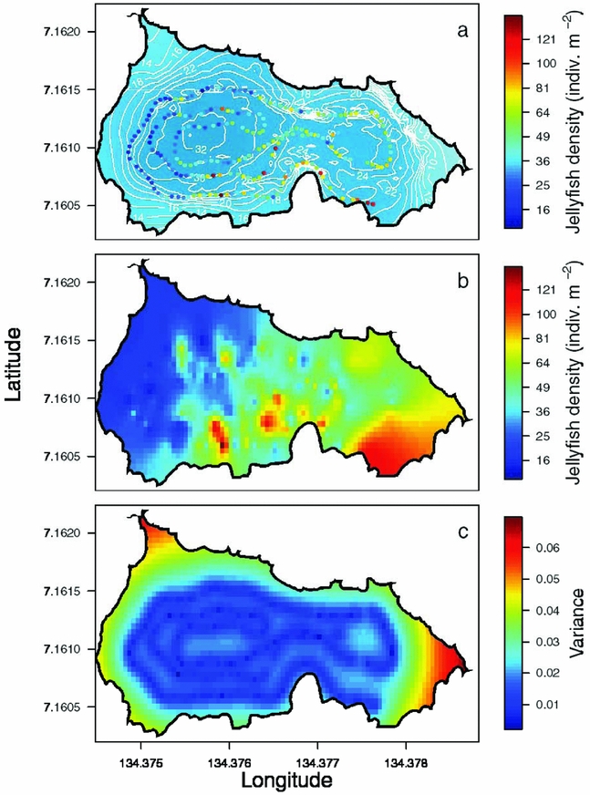
Appendix 2. An example of the interpolation process for jellyfish (Mastigias papua etpisoni) density in Jellyfish Lake, Palau. Jellyfish density along the REMUS track with bathymetry in the background (a), jellyfish density estimated from ordinary kriging (b) and spatially explicit estimates of the variance in interpolated estimates (c).
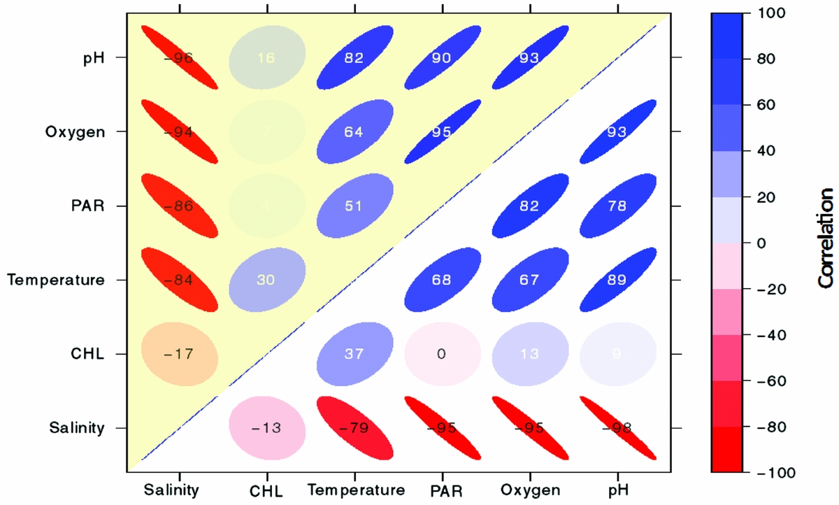
Appendix 3. Correlogram showing correlation coefficients using Pearson's correlation between the vertical distributions of physical and biological parameters (pH, oxygen, PAR (photosynthetically available radiation), temperature, CHL (chlorophyll-a) and salinity) in Jellyfish Lake, Palau. Colour and intensity of shading reveal the correlation where warm colours indicate a negative correlation and cool colours indicate a positive relationship. Circles indicate a low relationship whereas ellipses indicate a stronger relationship. For legibility, the values range from −100 to 100 but can be interpreted as Pearson's correlation, which ranges from −1 to 1. Correlations between variables on the east side of the lake are shaded yellow and variables on the west side of the lake are white.
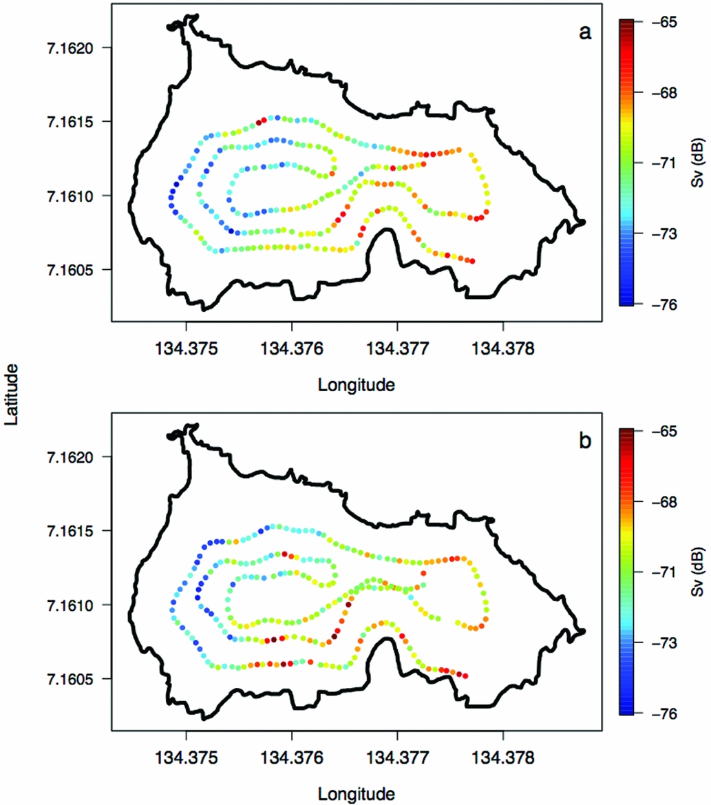
Appendix 4. Volume backscattering (Sv) of jellyfish (Mastigias papua etpisoni) along the REMUS track for missions 1 (a) and 2 (b) in Jellyfish Lake, Palau.