INTRODUCTION
Manta birostris (Walbaum, Reference Walbaum1792) is an exceptional ray species on account of its size, with some individuals measuring up to 9 m in width. They occur worldwide in tropical and subtropical regions, and occasionally migrate to temperate waters (Bigelow & Schroeder, Reference Bigelow, Schroeder, Bigelow and Schroeder1953; Compagno, Reference Compagno and Hamlett1999). While mantas are observed primarily in productive coastal areas near shore environments, they are also found at seamounts and even encountered far from shore in the open sea (Dewar et al., Reference Dewar, Mous, Domeier, Muljadi, Pet and Whitty2008; Luiz et al., Reference Luiz, Balboni, Kodja, Andrade and Marum2009; Marshall, Reference Marshall2009). Given the exceptional size of this species, it is very surprising that so little information exists about its biology. The lack of publications is partially due to the absence of industrial fishing for mantas as well as the minimal systematic collection of data. Information on growth rates, gestation period, age at sexual maturity and reproductive rates is scarce (Bigelow & Schroeder, Reference Bigelow, Schroeder, Bigelow and Schroeder1953; White et al., Reference White, Giles and Dharmadi2006).
Although not the target of large-scale fisheries, giant mantas are incidentally captured and/or taken in regional fisheries through much of their range (Alava et al., Reference Alava, Dolumbaló, Yaptinchay, Trono, Fowler, Reed and Dipper2002; White et al., Reference White, Giles and Dharmadi2006). Concerns about overexploitation resulted in listing the giant manta as Vulnerable in part of its range by the IUCN World Conservation Union (Marshall et al., Reference Marshall, Ishihara, Dudley, Clark, Jorgensen, Smith and Bizzarro2006). While elasmobranchs are generally considered highly susceptible to overfishing due to their natural history (Musick, Reference Musick1999), mantas are likely at an even greater risk given their very low reproductive rates, generally small population sizes and potentially limited distributions (Marshall et al., Reference Marshall, Ishihara, Dudley, Clark, Jorgensen, Smith and Bizzarro2006). A decline in manta sightings has been noted in a number of locations including Japan, French Polynesia and Mexico (Homma et al., Reference Homma, Maruyama, Itoh, Ishihara, Uchida, Seret and Sire1999; Marshall et al., Reference Marshall, Ishihara, Dudley, Clark, Jorgensen, Smith and Bizzarro2006).
Some of the best information available on distribution patterns within the mantas’ broad geographic range comes from photo identification studies that record the occurrence of photographically identified individuals over time. Based on this and other research, local residence patterns appear to be site-dependent (Dewar et al., Reference Dewar, Mous, Domeier, Muljadi, Pet and Whitty2008). In certain regions, the same individual mantas are observed repeatedly over long time periods (e.g. Yap, Hawaii and Bora Bora), whereas in others (e.g. New Zealand, parts of Australia, Baja California, Mexico, Africa, Ecuador and southern Japan), their occurrence is seasonal (Homma et al., Reference Homma, Maruyama, Itoh, Ishihara, Uchida, Seret and Sire1999; Duffy & Abbott, Reference Duffy and Abbott2003). When mantas are sighted on multiple occasions, they are often returning to the same feeding and cleaning stations (Homma et al., Reference Homma, Maruyama, Itoh, Ishihara, Uchida, Seret and Sire1999). Notarbartolo di Sciara & Hillyer (Reference Notarbartolo di Sciara and Hillyer1989) reported evidence of seasonality in the abundance and distribution of manta rays in the Caribbean Sea off Venezuela.
In 2006, 12 aerial surveys of French Guiana waters were undertaken (three per month in April, May, June and July). No M. birostris were observed until the first flight in July (11 July 2006) when around 50 individuals were seen together in one group (5°16′N 52°34′W) dispersed over 20 km2 and all swimming in a north-west direction (Girondot & Ponge, Reference Girondot and Ponge2006). None was observed on 12 July 2006, and only five were seen on 13 July. Such a migration was never before reported in this region. In 2008, 111 individuals were seen mainly along the continental shelf during another aerial survey campaign in French Guiana waters from 28 September to 12 October (Van Canneyt et al., Reference Van Canneyt, Certain, Dorémus and Ridoux2009). The authors reported an exceptional concentration (date and number not indicated) of M. birostris observed during one flight to the west of the continental shelf. However, each marine zone was surveyed only once (Mannocci et al., Reference Mannocci, Monestiez, Bolaños-Jiménez, Dorémus, Jeremie, Larand, Rinaldi, Van Canneyt and Ridoux2013), and it was not possible to conclude if the aggregation was geospatially stable or dependent on some temporal or trophic condition at sea, as previously proposed in Venezuela or Brazil (Notarbartolo di Sciara & Hillyer, Reference Notarbartolo di Sciara and Hillyer1989; Luiz et al., Reference Luiz, Balboni, Kodja, Andrade and Marum2009).
This unexpected pattern formed the basis of a programme for monitoring this species as part of a more general programme undertaken in French Guiana waters in the context of an environmental impact assessment prior to oil drilling.
MATERIALS AND METHODS
Aerial survey
From 15 September 2009 to 2 September 2011, 117 aerial surveys of the marine environment were conducted in French Guiana waters (South America) as part of an impact assessment for oil drilling (18, 51 and 48 flights in 2009, 2010 and 2011, respectively). Five types of aerial surveys were conducted depending on the various objectives of the surveys (Figure 1A–E). The combined aerial surveys are shown in Figure 1F, with a grid of 0.1° × 0.1° shaded according to the number of times each square was monitored.

Fig. 1. Tracks of the five kinds of aerial surveys performed in French Guiana (A–E) and the superposition of all tracks taken from the 117 aerial surveys conducted from 2009 to 2011 with a shaded scale for each 0.1° × 0.1° square depending on the number of times the square was monitored. The south-east–north-west plain line indicates the continental shelf position. The dot and cross along the coast respectively mark the position of Cayenne and Kourou cities.
Aerial surveys were conducted at a height of 300 m. Two pilots and two observers were present in the plane for each survey. Prior to each flight, we requested meteorological information, and if the weather was not favourable in the survey zone, the flight was postponed until better observation conditions were obtained. The real-time position of the plane was recorded using Garmin GPS. Furthermore, information about weather and sea conditions was taken throughout the entire flight.
Each time an animal was observed (ray, shark, turtle or cetacean), the following information was recorded: time, GPS position, flight altitude, angle between the observed animal and the vertical, taxonomic identification of the individual at the most precise level, and behavioural information including the swimming direction. A circle-back procedure was then applied to 26 animals (Hiby, Reference Hiby, Garner, Amstrup, Laake, Manly, McDonald and Robertson1999) in the following manner: the pilot continued the flight for 30 s, then made a half-circle and returned parallel to the original line for 1 min, before finally making a second half-circle, with the zone where the animal was seen being monitored again. This is one approach for estimating the detection probability of animals. Photos were subsequently taken when possible using a zoom of 300% to ensure their identification at the end of the mission.
Systematics and identification
Devil rays (Family Mobulidae, Suborder Myliobatoidei, Order Rajiformes, Subclass Elasmobranchii, Class Chondrichthyes) are currently divided into two distinctive genera: Mobula Rafinesque, 1810 and Manta Bancroft, 1828. The genus Manta contains two species: the reef manta ray Manta alfredi (Krefft, Reference Krefft1868) and the giant manta ray Manta birostris (Walbaum, Reference Walbaum1792), which is the largest ray in the world. Long considered to be the same species, the status of the reef manta ray as a separate species was only confirmed in 2009 (Marshall, Reference Marshall2009). A third form, termed Manta sp. cf. birostris, was differentiated in the specimens examined and photographed in the Atlantic Ocean and Caribbean, but further evidence is needed to elucidate its taxonomic status (Marshall, Reference Marshall2009).
Reef manta rays are typically 3–3.5 m in disc width with a maximum size of about 5.5 m, while M. birostris has a common length of 4.5 m (Stehmann, Reference Stehmann, Fischer, Bianchi and Scott1981) and reaches disc widths of at least 7 m (Last & Stevens, Reference Last and Stevens2009) with anecdotal reports up to 9.1 m (Compagno, Reference Compagno and Hamlett1999; White et al., Reference White, Giles and Dharmadi2006).
These two species of manta rays are the largest in the family Mobulidae and indeed the largest rays in the world. The dorsal surface is black, with large, conspicuous, white shoulder patches in the suprabranchial region, with or without black spots inside them (Figure 2). Manta rays have a distinctive body shape with triangular ‘wings’ and paddle-like lobes extending in front of their mouths. The disc is approximately 2.2–2.3 times as broad as it is long. The animal has a slender, whip-like tail that exceeds the disc length if intact. Marshall (Reference Marshall2009) identified a total of 10 non-overlapping proportional measurements that could be used to distinguish the M. birostris from the M. alfredi. However, the distinction between the M. alfredi and M. birostris based on measurements taken from aerial photography is not reliable enough to be used. Nevertheless, M. alfredi is mainly an Indo-Pacific species, observed sporadically in eastern Atlantic waters, but never in the west Atlantic (Marshall, Reference Marshall2009). Although we cannot be entirely sure that the individuals observed were indeed M. birostris, only this species occurs in French Guiana based on current knowledge.

Fig. 2. Manta birostris, 25 September 2010 (picture taken at an altitude of 300 m).
Ocean net primary production
Net primary production (NPP) is commonly modelled as a function of chlorophyll concentration. However, it has long been recognized that variability in intracellular chlorophyll content from light acclimation and nutrient stress confounds the relationship between chlorophyll and phytoplankton biomass. To account for this effect, the carbon-based productivity model (CbPM) was first described by Behrenfeld et al. (Reference Behrenfeld, Boss, Siegel and Shea2005) and has since been expanded to model spectral differences in light penetration through the euphotic zone (Westberry et al., Reference Westberry, Behrenfeld, Siegel and Boss2008). The CbPM was therefore used here as a proxy of NPP.
Data analysis
GENERALIZED LINEAR MIXED MODEL
Flight survey data were grouped in a square of 0.1° × 0.1° (note that this surface is not precisely a square in kilometres, but the difference between squares in the studied zone is very small, <0.01 km2). The use of the 0.1° × 0.1° square as opposed to the kilometre square was necessary in order to be coherent with the sea surface temperature (SST) and NPP data. For each flight, the surface monitored in each square was computed based on the GPS real-time track by multiplying the linear distance in each square by the mean altitude of the survey in that square. The rationale for this was that observations were only possible on the side opposite the position of the sun, while the maximum angle to observe individuals was 45° (see Van Canneyt et al., Reference Van Canneyt, Certain, Dorémus and Ridoux2009). The number of observations of M. birostris for each square and each flight was then enumerated. The SST for each square and day of flight was also computed (Reynolds et al., Reference Reynolds, Smith, Liu, Chelton, Casey and Schlax2007).
The number of sightings per 0.1° × 0.1° square was fitted using a generalized linear mixed model (GLMM). The random factor was the flight identity, while the fixed factors were the periodic effect based on the ordinal day in the year (sDays = sin(2π day)/365.25, cDays = cos(2π day)/365.25), the distance from the middle of the square to the nearest coast line and to the continental slope at a depth of 1000 m, SST, NPP and the surface prospected in each square. First-order interactions were also included in the model. Zero-inflated Poisson distribution with log link was used to fit data using penalized quasi-likelihood. When the factors involved the periodic effect based on the ordinal day in the year (sDays and cDays), the significance of the factor used the z-transformed combined probability of each single factor (Whitlock, Reference Whitlock2005). Backward model selection was performed by removing at each step the least significant factor until only significant ones remained (P < 0.05; factor was retained if used in a significant interaction). Models were run using the glmmPQL function in the MASS package in R (Venables & Ripley, Reference Venables and Ripley2002). The names of the factors are as follows:
-
– Passage: Prospected surface in km2 within the 0.1° × 0.1° square;
-
– cDays and sDays: Periodic effect based on the ordinal day in the year;
-
– Coast: Minimum distance in km from the centre of the 0.1° × 0.1° square to the coast line;
-
– Slope: Minimum distance in km from the centre of the 0.1° × 0.1° square to the line of middle slope;
-
– SST: Sea surface temperature in °C within the 0.1° × 0.1° square;
-
– NPP: Square root of the net primary production in mg C m−3 d−1 within the 0.1° × 0.1° square.
Parametric phenology model
To ensure that the pattern of periodicity detected by GLMM was not too constrained by the model construction itself, the number of ray sightings per flight was fitted using the methodology developed by Girondot (Reference Girondot2010). In short, a non-linear function is fitted onto the counts using maximum likelihood with negative-binomial distribution. The non-linear function uses six parameters that have a direct phenological interpretation:
-
– Min: Basal number of observations (different each year);
-
– Max: Mean number of observations per flight at the peak of the season (different each year);
-
– Peak: Ordinal day at the peak of the season (identical every year);
-
– LengthB: Length of the season before Peak (identical every year);
-
– LengthE: Length of the season after Peak (identical every year);
-
– Theta: Negative-binomial parameter describing dispersion around the mean.
The model was compared to a constant model using the Akaike information content (AIC) (Akaike, Reference Akaike1974). AIC is a ranking measure that takes into account the quality of the model fit by comparing it with the data while penalizing the number of parameters used:
 $${\rm AIC=} - {\rm 2ln}\, L+2\, M$$
where L corresponds to the maximum likelihood and M to the number of parameters. Models with the lowest AIC values were retained as good candidate models and ΔAIC was calculated as the difference in AIC value between a particular model and the one with the lowest AIC. Akaike weights (w i = exp(−ΔAIC/2) normalized to 1) were used to evaluate the relative support of the various tested models (Burnham & Anderson, Reference Burnham and Anderson1998). Akaike weights can be directly interpreted as conditional probabilities for each model. Ideally, the model with the lowest AIC was kept for further testing. When two or more models possessed similar Akaike weights, the model with the lowest number of parameters was selected. When several models had the same number of parameters, the model with the lowest AIC was chosen.
RESULTS
Overall, 117 flights were performed covering a total of 111,094 km linear distance (18,196 km in 2009, 52,901 km in 2010 and 39,996 km in 2011). The distribution of the monitored surface per 0.1° × 0.1° square shows a mode at 2.92 km2 based on the method of Asselin de Beauville (Reference Asselin de Beauville1978). Among these 117 flights, M. birostris was observed in 54 of them (46.15%) for a total of 138 individuals.
GLMM analysis
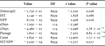
The final selected model for the spatial and temporal distribution of M. birostris is shown in Table 1. As expected, the ‘passage’ factor, which is the prospected surface within the 0.1° × 0.1° square, is highly significant. The higher the prospected surface within the square is, the higher the probability to observe a ray. The distance to the coastline is also highly significant, revealing that rays are more present at the centre of the continental shelf (Figure 3). The pair of cDays and sDays is also highly significant, which indicates that a very significant periodicity is observed with a peak presence in early September and the lowest in March (Figure 3). However, it should be noted that the methodology used here constrains the periodicity to be perfectly symmetric around the peak, which would obviously not represent reality (see below).

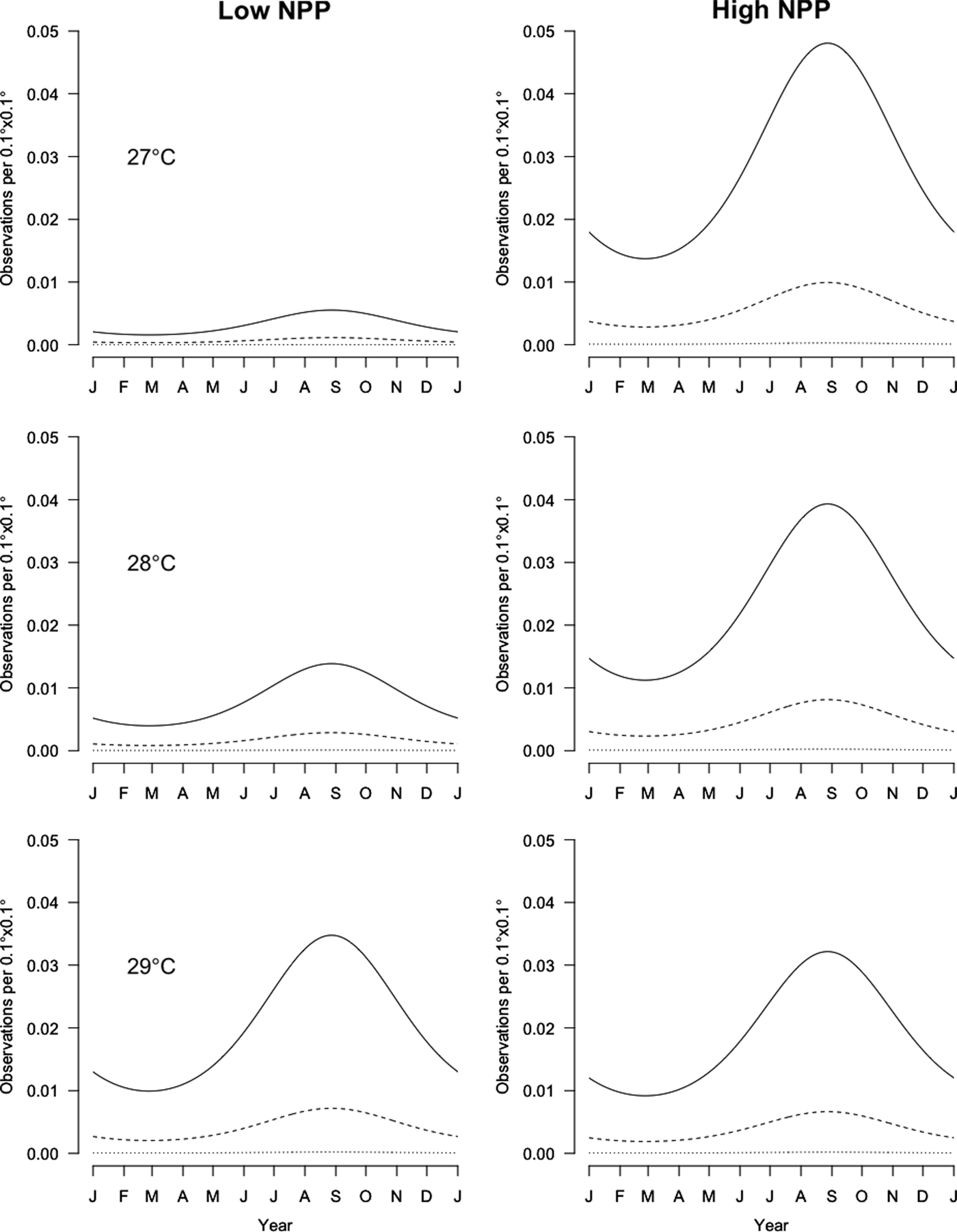
Fig. 3. Prediction of the number of observations per 0.1° × 0.1° square for the selected model depending on the surface sea temperature (SST) (27, 28 and 29°C), low and high net primary production (NPP) (100 and 4900 mg C m−3 d−1, respectively), day of the year and spatial position (continental shelf: coast = 84 km, slope = 67 km; slope: coast = 137 km, slope = 24 km). The surface monitored per square is set as the mode of the monitored surfaces per square: 2.925 km2. Plain curves are in the middle of the continental shelf, dashed curves are located in the middle of the slope, and dotted lines are for oceanic localization.
Table 1. Significance of different factors involved in the generalized linear mixed model (GLMM) after backward selection. The P value shown for factors involving sDays and cDays is based on the combined probabilities using z-transform (Whitlock, Reference Whitlock2005).

The next significant factors are the SST, NPP and their interaction. It should be noted that the SST and NPP are not independent from the month of the year or from the distance to the coast. However, as these factors are also retained in the analysis, this indicates that the effects of SST and NPP are detected beyond their annual and spatial variability.
The higher the SST and NPP are, the more rays are detected (Figure 3). At 29°C, rays are detected regardless of the NPP, but they are much less frequently detected at 27°C except if the NPP is high.
Parametric phenology analysis
The constraint of the symmetric periodic pattern across the year was relaxed using the methodology developed by Girondot (Reference Girondot2010) in order to fit a periodic pattern onto a time series of counts. The selected model (periodic vs constant, Akaike weight = 0.998) shows a rapid increase in the presence of rays from May to July, followed by a relatively flat period from July to September and a slow decrease from September to January (Figure 4). However, this analysis does not allow for the effect of all other factors, notably the length of the aerial survey and its position relative to the coast. Nevertheless, no significant relationship between the survey month and the total length of the aerial transects was observed (t = 0.01, df = 115, P = 0.99).

Fig. 4. Periodicity of the number of rays observed during flights modelled using the parametric equation from Girondot (Reference Girondot2010). The dots indicate the observed number of individuals per flight, the plain line the average number of individuals, the dashed lines the 95% confidence interval for the average number of individuals, and the dotted lines the 95% confidence interval for the number of observations per flight based on negative binomial distribution.
Circle-back procedure
The circle-back procedure was applied to 26 of the 138 observations. In all of these cases, the individual was observed again at the second passage. Thus, the probability of detecting an animal that is indeed present in the aerial transect is very high (CI 95% from 0.87 to 1) (based on the Wilson score test, see Agresti & Coull, Reference Agresti and Coull1998).
DISCUSSION
Many mysteries remain about the basic life history of manta rays. For example, it is uncertain how many exchanges take place between different stocks or whether the populations in different oceans may actually be separate species (Shark Specialist Group of the IUCN Species Survival Commission, 2007).
The seasonality of the presence of manta rays is also poorly understood. In Komodo Island, Indonesia, the most popular site for observing mantas is situated off the southern tip of Komodo Island in an area with a high degree of bathymetric structure. An examination of the longest records suggests some site preference, with five of seven individuals spending more than 90% of their time at the location where they were tagged. The strongest seasonal pattern was observed in the south where no mantas were recorded in the first quarter of any year. This coincides with an increase in temperatures and a reduction in productivity in this region as associated with monsoonal shifts (Dewar et al., Reference Dewar, Mous, Domeier, Muljadi, Pet and Whitty2008).
Underwater photographs of M. birostris gathered over a period of 9 years in a marine protected area in southeastern Brazil suggest a high predictability of manta ray occurrences in the region during the austral winter (June–September). The reasons for this are probably related to the seasonal oceanographic conditions, as characterized by the presence of a coastal front at the study site in winter and the consequent plankton enrichment, which provides a feeding opportunity for manta rays (Luiz et al., Reference Luiz, Balboni, Kodja, Andrade and Marum2009).
The pattern that we detected in French Guiana reveals an increase in the presence/detectability of manta rays from May to January in both the GLMM and the parametric models. As the observations were conducted from aerial surveys with most being done at a depth of >10 m in cloudy water, it is still possible that undetected animals were present below the surface. The detected temporal difference could be dependent on feeding behaviour as well as migratory patterns. We cannot completely eliminate this possibility but two observations lead us to prefer the migratory hypothesis: first, the observation of a large number of manta rays all swimming in the same direction on one particular day; and second, the very high probability detection, indicating that this species spends lengthy periods at the surface. The ideal situation would be to analyse these data using a combination of a parametric model and cofactors in the analysis in order to take advantage of both methodologies, but statistical tools permitting such an analysis are still not available.
Link with ocean productivity
Manta rays are filter feeders, hence their modified branchial apparatus. They mainly feed on all kinds of planktonic crustaceans in addition to small schooling fish. Therefore, local oceanic productivity may be a key to understanding the periodicity detected in relation to this species’ presence in French Guiana waters.
Two factors are essential to understanding the marine hydrology in French Guiana: its location to the north of the equator and the presence of the Amazon River located 500 km to the south. The Amazon is the largest river system in the world, contributing about 6 × 10¹² m3 of fresh water to the tropical Atlantic each year. This is about 16% of the annual discharge into the world's oceans (Gibbs, Reference Gibbs1970).
Systems of currents and countercurrents guide the hydrography in front of French Guiana (Muller-Karger et al., Reference Muller-Karger, Mcclain and Richardson1988). The equatorial currents directed from east to west around the equator are located at 10°N (north equatorial current) and from 5°S to 2°N (south equatorial current). The north equatorial countercurrent is located between these currents. When reaching the South American coast, the south equatorial current separates into two branches: the Brazil current toward the south-west and the North Brazil current toward the north-west. During the first half of the year, the North Brazil current becomes the Guyana current, and Amazonian water is exported toward the Caribbean Sea, extending over a broad geographic area that includes a coastal turbid zone, a large river plume and offshore lenses of low-salinity water. From July to December, the Guyana current bifurcates between 5°N and 8°N, and then Amazon water is retroflected into the north equatorial countercurrent (Muller-Karger et al., Reference Muller-Karger, Mcclain and Richardson1988) in front of the French Guianan coast as a result of increased south-east trade winds. As a consequence, a large amount of sediment from the Amazon River is exported to the east (Hu et al., Reference Hu, Montgomery, Schmitt and Muller-Karger2004), while the water in French Guiana is generally calm and less turbid (Pujos & Froidefond, Reference Pujos and Froidefond1995; Froidefond et al., Reference Froidefond, Gardel, Guiral, Parra and Ternon2002; Baklouti et al., Reference Baklouti, Devenon, Bourret, Froidefond, Ternon and Fuda2007).
Along with fresh water, the Amazon provides the largest riverine flux of suspended (1200 Mt y−1) and dissolved matter (287 Mt y−1), which includes a dissolved organic matter flux of 139 Mt y−1 (Meybeck & Ragu, Reference Meybeck and Ragu1997). These fluxes can have a dramatic effect on regional ecology as they represent potential subsidies of organic carbon, nutrients and light attenuation in an otherwise oligotrophic environment (Muller-Karger et al., Reference Muller-Karger, Mcclain and Richardson1988). Both chlorophyll (Chl) concentration and primary productivity on the continental shelf are the highest in the river–ocean transition zone, where the bulk of heavy sediments settle out of surface waters (Smith & Demaster, Reference Smith and Demaster1996). The combination of riverine nutrient input and increased irradiance availability creates a highly productive transition zone, the location of which varies with the discharge from the river. Phytoplankton biomass and productivity of over 25 mg Chl-a m−3 and 8 g C m−2 d−1, respectively, are found in this transition region (Smith & Demaster, Reference Smith and Demaster1996). Increased irradiance from July to December in the continental shelf of French Guiana (Pujos & Froidefond, Reference Pujos and Froidefond1995; Froidefond et al., Reference Froidefond, Gardel, Guiral, Parra and Ternon2002; Baklouti et al., Reference Baklouti, Devenon, Bourret, Froidefond, Ternon and Fuda2007) could be linked to increased primary production. This period corresponds to the highest presence in manta rays in French Guiana.
Although the temporality of the manta rays’ presence in French Guiana seems well established, their location from January to July still remains unknown. First, it should be noted that some individuals are seen throughout the entire year. Thus, even if a migration pattern does exist, it is not generalized. Second, an exceptional number of individuals were seen on 11 July 2006, all swimming in the same north-westerly direction in a movement that resembled a migration. We can therefore propose that they were closer to the equator and moving toward French Guiana waters at the period of the highest productivity in this area.
We prefer not to provide the number of individuals present in French Guiana waters due to the high uncertainty resulting from the lack of knowledge in detection probability and the comprehension of movement patterns. We can only say that the number of individuals present at the same time in French Guiana waters was greater than 50, which is the maximum number of individuals observed in a single flight in 2006.
ACKNOWLEDGEMENTS
This research was made possible thanks to the investment of Tullow Oil PLC, which financed and organized all of the logistics for the 117 aerial surveys. We particularly wish to acknowledge Joachim Vogt. We would also like to thank the two pilots, Laurent and Philippe Bénibri, for their continuous help and interest in this work. NOAA_OI_SST_V2 data provided by the NOAA/OAR/ESRL PSD, Boulder, Colorado, USA, from their Web site at http://www.esrl.noaa.gov/psd/. The manuscript has benefited from the corrections of Mrs Victoria Grace (English publications service).