INTRODUCTION
The Southern California Bight (SCB) is a highly populated (~20 million people) area that extends from Point Conception in southern California to the south of Ensenada, Baja California, Mexico (Macías-Zamora et al., Reference Macías-Zamora, Ramírez-Álvarez and Sánchez-Osorio2014a). This is an important and unique region with large marine ecosystem resources, and a history of organic sediment pollution from an increasing human population resulting in substantial environmental stress (Schiff et al., Reference Schiff, James Allen, Zeng and Bay2000; Dodder et al., Reference Dodder, Lauenstein, Ramirez, Ritter, Maruya and Schiff2011). Due to weather conditions in the region, pollutants can build up on impervious surfaces during the extended dry season, and subsequently washed off into the ocean once the wet season begins. Atmospheric deposition may be especially important as a source of pollutants in stormwater effluents in this region. Significant quantities of trace metals and other pollutants are emitted into the atmosphere daily, followed by deposition in the water column, rapid removal and transportation to bottom sediments (Chong & Wang, Reference Chong and Wang2000; Schiff et al., Reference Schiff, James Allen, Zeng and Bay2000; Sabin et al., Reference Sabin, Jeong, Stolzenbach and Schiff2005; Castro-Morales et al., Reference Castro-Morales, Macías-Zamora, Canino-Herrera and Burke2014; Macías-Zamora et al., Reference Macías-Zamora, Ramírez-Álvarez and Sánchez-Osorio2014a, Reference Macías-Zamora, Ramírez-Álvarez, Hernández-Guzmán and Mejía-Trejo2016). These anthropogenic contaminants may accumulate in sediments of nearshore coastal regions causing habitat alteration and thus changes in community composition, abundance and diversity of benthic fauna (Lenihan et al., Reference Lenihan, Peterson, Kim, Conlan, Fairey, McDonald and Oliver2003; Ranasinghe et al., Reference Ranasinghe, Montagne, Smith, Mikel, Weisberg, Cadien, Velarde and Dalkey2003, Reference Ranasinghe, Barnett, Schiff, Montagne, Brantley, Beegan, Cadien, Cash, Deets, Diener, Mikel, Smith, Velarde, Watts and Weisberg2007, Reference Ranasinghe, Schiff, Brantley, Lovell, Cadien, Mikel, Velarde, Holt and Johnson2012).
Polychaetes are good representatives of benthic communities because they are often the dominant taxa in terms of abundance, biomass and species composition in soft-bottom sediments. They play a major functional role in recycling, reworking and bioturbation of marine sediments as well as the burial of organic matter (Hutchings, Reference Hutchings1998). Polychaetes may, therefore, be good indicators of community patterns in benthic invertebrate assemblages, not only because of their high abundances, but also their high diversity of feeding guilds, and their ability to adapt and occupy a whole environmental range of habitats (Fauchald & Jumars, Reference Fauchald and Jumars1979; Mackie & Oliver, Reference Mackie, Oliver and Hall1996; Giangrande et al., Reference Giangrande, Licciano and Musco2005).
The SCB is a region widely studied in the USA. In contrast, the north-western Pacific coast of Mexico is an area little studied, with no integration of regional temporal variability in the benthic environment. Rodríguez-Villanueva et al. (Reference Rodríguez-Villanueva, Martinez-Lara and Macías-Zamora2003) carried out a baseline survey designed to evaluate benthic invertebrates and their possible relationship with environmental variables in the north-western coast of Mexico. Following this study, other regional surveys on persistent organic pollutants in marine sediments have been published in this region (Macías-Zamora & Canedo-López, Reference Macías-Zamora and Canedo-López2008; Macías-Zamora et al., Reference Macías-Zamora, Sanchez-Osorio, Ramírez-Álvarez and Ríos-Mendoza2008a, Reference Macías-Zamora, Ramírez-Álvarez and Sánchez-Osorio2014a, Reference Macías-Zamora, Ramírez-Álvarez and Hernández-Guzmánb, 2016) but none concerning marine invertebrates and their relationship with the environment. The objective of this study was to provide a regional perspective of the changes (both spatial as well as temporal) in the benthic community using polychaetes as a surrogate measure of environmental conditions, and to establish a temporal comparison between El Niño-Southern Oscillation (ENSO), ENSO-drought conditions and polychaete assemblages over the last 15 years.
MATERIALS AND METHODS
Study area
The study area encompasses the coastal shelf waters of the north-western region of Baja California, between 32.549°N 117.333°W and 31.751°N 116.639°W. It is limited to the north by the Pacific Ocean extension of the USA–Mexico International border, to the south by Punta Banda, Baja California, and to the west by the 200 m isobath (Rodríguez-Villanueva et al., Reference Rodríguez-Villanueva, Martinez-Lara and Macías-Zamora2003) (Figure 1). The SCB extends from Point Conception, California, USA to Cabo Colonet in Baja California, Mexico. Three-quarters of the mainland shelf Bight is in the USA (3795 km2), while the rest is located on the north-western coast of Mexico (1300 km2).

Fig. 1. Sampling sites for benthic macrofauna (polychaetes) and sediment on the north-western coast of Baja California, Mexico. The isobath of 200 m depth is indicated.
Field sampling design
Following the baseline survey of Rodríguez-Villanueva et al. (Reference Rodríguez-Villanueva, Martinez-Lara and Macías-Zamora2003) the study area was subdivided into three arbitrary zones (north, centre and south) (Figure 1) in parallel with the influence of two discontinuous industrialized population centres, as follows:
The northern zone extends from the USA–Mexico border (Pacific Ocean borderline) to Punta Descanso. It is characterized by its proximity to the largest population centres in Mexico (Tijuana and Rosarito B.C.) and the USA (San Diego, CA). This zone is characterized by a wide continental platform and is influenced by Tijuana Estuary, and the Binational and Punta Bandera wastewater treatment plants, and to a lesser extent by the Point Loma wastewater treatment plant.
The centre zone extends from Punta Descanso in the north to Punta Salsipuedes to the south. It is considered as a control area given the reduced population and absence of wastewater treatment plants (Macías-Zamora et al., Reference Macías-Zamora, Ramírez-Álvarez and Sánchez-Osorio2014a). This zone is influenced by the natural discharge of La Misión creek and has a narrow continental platform. Carter (Reference Carter1988) and Serrano-López (Reference Serrano-López1999) characterized this zone as an open bay.
The south zone includes the second largest city, Ensenada Baja California. It also includes Salsipuedes Bay, Todos Santos Bay and Punta Banda Estuary. It has a wide continental platform influenced by the discharges of three wastewater treatments plants (El Sauzal, El Gallo and El Naranjo).
Data collection
Sediments were sampled during three different ENSO events with corresponding intensity conditions, from the research vessels ‘Alguita’ and ‘Suchiate’ during three oceanographic cruises. In September 1998 during a strong ENSO event (‘Bight 98’), 72 stations were sampled; in December 2003 after a weak ENSO event (‘Bight 03’) 66 stations were sampled, and finally in October 2013 during regional drought conditions (‘Bight 13’) 80 stations were sampled. The stations were sampled using a van Veen (0.1 m2) grab at depths ranging between 15 to 206 m (Figure 1). To define the sample stations a ‘multiple density nested random-tessellation stratified design (MD-NRTS)’ was utilized (Stevens, Reference Stevens1997). MD-NRTS is a method used for populations distributed in a continuous fashion that measures environmental conditions at a regional scale. This method is based on a random stratified design that considered three strata: depth (I = 6–30 m, II = 31–120 m and III = 121–200 m), continental platform amplitude, and proximity to potential sources of anthropogenic impact.
Two grabs were taken per station, the first to analyse the macrofaunal community, and the second to analyse the chemical characteristics of the sediment. Macrofauna samples were sieved onboard through a 1.0 mm mesh screen, and all retained organisms placed in labelled plastic containers, relaxed for 30 min in MgSO4 solution, and later fixed in 10% borax-buffered formalin.
Sample treatment
In the laboratory, each macrofauna sample was washed with fresh water through a 0.5 mm mesh sieve and retained macroinvertebrates sorted in a Petri dish in 70% ethyl alcohol under a stereoscopic microscope. For this study, all polychaetes were separated, classified and later identified to family level with the use of keys and specialized literature (Fauchald, Reference Fauchald1977; Blake et al., Reference Blake, Hilbig and Scott1997; Rouse & Pleijel, Reference Rouse and Pleijel2001; de León-González et al., Reference de León-González, Bastida-Zavala, Carrera-Parra, García-Garza, Peña-Rivera, Salazar-Vallejo and Solís-Weiss2009).
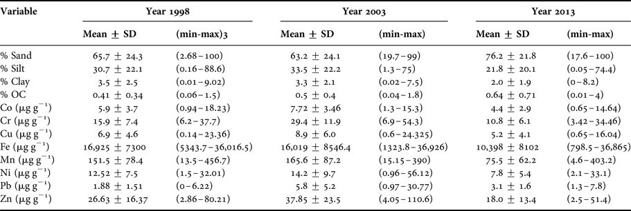
Three subsamples of sediment from the chemistry grabs were collected to determine the fine fraction (% <63 µm), organic carbon content (%OC), and trace metal concentrations. All samples were collected using a Teflon spatula, stored in previously acid-washed polypropylene centrifuge flasks, and kept frozen until further analysis. For measurements of trace metal concentrations, the sediment samples were digested and processed according to the method reported by Macías-Zamora et al. (Reference Macías-Zamora, Sánchez-Osorio, Ríos-Mendoza, Ramírez-Álvarez, Huerta-Díaz and López-Sánchez2008b). The analysis included the following trace metals: Co, Cr, Cu, Mn, Ni, Pb and Zn all in units of μg g−1 dry weight, as well as Fe (μg g−1) as a normalizing agent. Quantification was made using an Agilent 240FS AA fast sequential atomic absorption spectrometer. Sediment grain size distribution (GS) (% <63 µm) was determined using a Horiba (model LA-910) laser/tungsten particle size analyser according to the methodology described by Daesslé et al. (Reference Daesslé, Ramos, Carriquiry and Camacho-Ibar2002). A LECO (model CHNS-932) elemental analyser was used to determine the percentage of OC (%OC) in the sediment samples (Schiff & Weisberg, Reference Schiff and Weisberg1999).
Data analysis
ENVIRONMENTAL VARIABLES
Descriptive statistics were utilized to analyse the environmental variables measured: depth (m), %OC, sediment grain size (% <63 µm) and trace metal characteristics including Co, Cr, Cu, Fe, Mn, Ni, Pb and Zn in μg g−1 dry weight. In order to identify metal enrichment, metal-Fe baselines were established. According to Schiff & Weisberg (Reference Schiff and Weisberg1999), baseline relationships represent the prediction, which is considered as a natural concentration; thus, any concentration above that baseline limit would represent enrichment. In this study, we followed the procedure described by Schiff & Weisberg (Reference Schiff and Weisberg1999) to create the baseline of trace metals for the three sampling campaigns: 1998, 2003 and 2013.
Multivariate analysis
Multivariate analyses of the data were carried out to measure the level of association of different sample sites. To understand the spatial distribution of environmental parameters, Euclidean distances coefficient was calculated based on environmental/abiotic data previously normalized, resulting in a correlation matrix of the 11 environmental variables previously mentioned. Principal components analysis (PCA) was applied to the correlation matrix, which included all of the sampling stations in every year sampled. The analysis was applied using various routines in PRIMER-E v6 software (Clarke & Gorley, Reference Clarke2006).
BENTHIC MACROFAUNA
Univariate analysis
Differences between the sampled sites at spatial and temporal scales were examined using univariate community parameters, such as abundance (organisms per 0.1 m2), family richness (S), Shannon–Wiener diversity index (H′ log2), and Pielou's evenness index (J’) (Pielou, Reference Pielou1977; Odum, Reference Odum1979; Frontier, Reference Frontier1985; Ludwig & Reynolds, Reference Ludwig and Reynolds1988). Shannon–Wiener diversity index can usually take values between 0 and 5 bits per individual (Marques et al., Reference Marques, Salas, Patricio, Teixera and Neto2009). Molvaer et al. (Reference Molvaer, Knutzen, Magnusson, Rygg, Skey and Sorensen1997) established the following relationship between Shannon–Wiener index values and different levels of ecological quality, in accordance with the Framework Directive (WFD, 2000/60/EC). High status H′ > 4 bits per individual; Good status 3 < H′ ≤ 4 bits per individual; Moderate status 2 < H′ ≤ 3 bits per individual; Poor status 1 < H′ ≤ 2 bits per individual; and Bad status ≤ 1 bits per individual In order to understand the spatial distribution of polychaete families that make up the communities within the area of study, they were ranked according to the frequency of appearance in each of the sites sampled, expressed as percentile against the abundance of organisms.
Multivariate analysis
To analyse the level of association or similarity of different sample sites, and detect spatial patterns among the composition and abundance of the polychaete community, ordination and classification methods were used. An ordination space non-metric multidimensional scaling (nMDS) was constructed on transformed data (square root), employing the Bray–Curtis similarity coefficient. Relationships within each nMDS were identified by cluster analysis using the group average method. Posteriorly a one-way analysis of similarity (ANOSIM) for differences among groups detected was utilized. In addition, a SIMPER analysis was carried out to identify which taxa were most responsible for similarities within groups. The analyses were applied using PRIMER-E v6 software (Warwick & Clarke, Reference Warwick and Clarke1991; Clarke, Reference Clarke1993; Clarke & Warwick, Reference Clarke and Warwick1994; Clarke & Gorley, Reference Clarke and Gorley2006).
Relationship to environmental parameters
Environmental variables, as well as the structure of the polychaete fauna were analysed using Bio-Env analysis, which selects a variable, or combination of variables which best explained the differences in polychaete community structure observed. Bio-Env analysis shows the maximum values for the range coefficient of the Spearman correlation. For the best combinations of one, two, three or more variables, coefficient values are near one when a good correlation exists, and near zero when there is a small, or no correlation (Clarke & Warwick, Reference Clarke and Warwick1994). For this analysis we used a similarity matrix constructed using the Bray–Curtis similarity coefficient. Family abundance data was initially square root transformed, and a similarity matrix constructed using Euclidean distances coefficient after normalizing the 11 environmental variables: depth (m), OC (%), sediment grain size <63 µm (%), and heavy metal characteristics Co (μg g−1), Cr (μg g−1), Cu (μg g−1), Fe (μg g−1), Mn (μg g−1), Ni (μg g−1), Pb (μg g−1) and Zn (μg g−1).
Spatio-temporal differences in community structure of polychaete families and environmental variables were evaluated using a factor design (including: ‘year’, ‘zone’) and a permutational multivariate analysis of variance (Permanova). This analysis was done using 1000 permutations in the PRIMER 6 and PERMANOVA+ package (Anderson et al., Reference Anderson, Gorley and Clarke2008). All Permanova tests were calculated using a two-factored design: Time (3 levels; fixed) and zone (3 levels; fixed).
RESULTS
Sediment characteristics
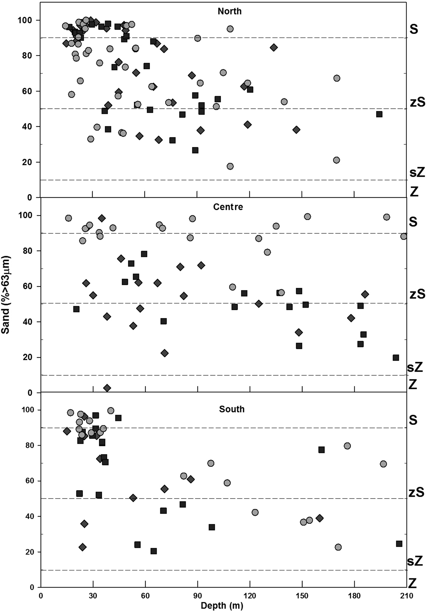
In general, sand predominated within the study area (Figure 2), representing on average more than 60%, while silt averaged between 20–30%, and clay less than 10%. However, in 1998 and 2003, the percentage of sand, silt and clay was found to be similar. In 2013, a decrease of the fine fraction (silt-clay) was observed in comparison to previous sampling years. Spatially, the inner shelf (6–30 m) was mainly sand (% >63 µm) (Figure 3), while on the middle shelf (31–121 m), the sediments varied between silty-sands and sandy-silts, with increased heterogeneity in grain size. On the outer shelf (121–200 m) sandy-silts were the predominant sediment. The clay (<4 µm) fraction had the lowest values observed, with content less than 10% in all samples. The inner shelf (6–30 m) for the north study area showed an increase in silt in 2013 that was not detected in 1998 or 2003. Other important changes occurred in the centre zone where the heterogeneity of the sediments decreased for 2013 when the sand content was highest (>80%) in the three shelf strata. In 1998 and 2003, the sand content in the centre zone varied between 20 and 98% in the three strata of the main shelf.
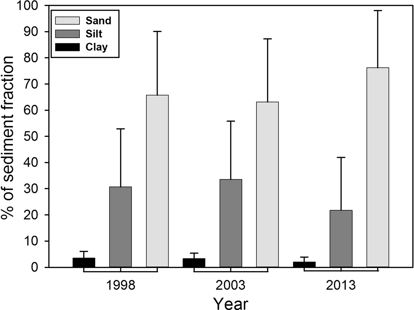
Fig. 2. Average per cent of the three main grain size fractions within the sampled sediments on the north-western coast of Baja California, Mexico. The SD for the three sampling years is shown by the whiskers.

Fig. 3. Sediment distribution: Sand (S), Silty-sand (zS), Sandy-silt (zS) and Silt (Z). Stations separated by zone and arranged by depth in each year. 1998 = ⋄, 2003 = □, 2013 = ○.
The average percentage of organic carbon (%OC) increased from 1998 to 2013 (Table 1). The correlation of the fine sediment fraction (% <63 µm) with the %OC was <0.5 for 1998 and 2003, but in 2013, there was no correlation between both variables because of the predominance of sands in the area. However, the overall tendency in the three sampling years was for %OC to increase with increased water depth.
Table 1. Values of environment variables in marine sediments from north-western coast of Baja California, Mexico.
CONCENTRATIONS OF METALS
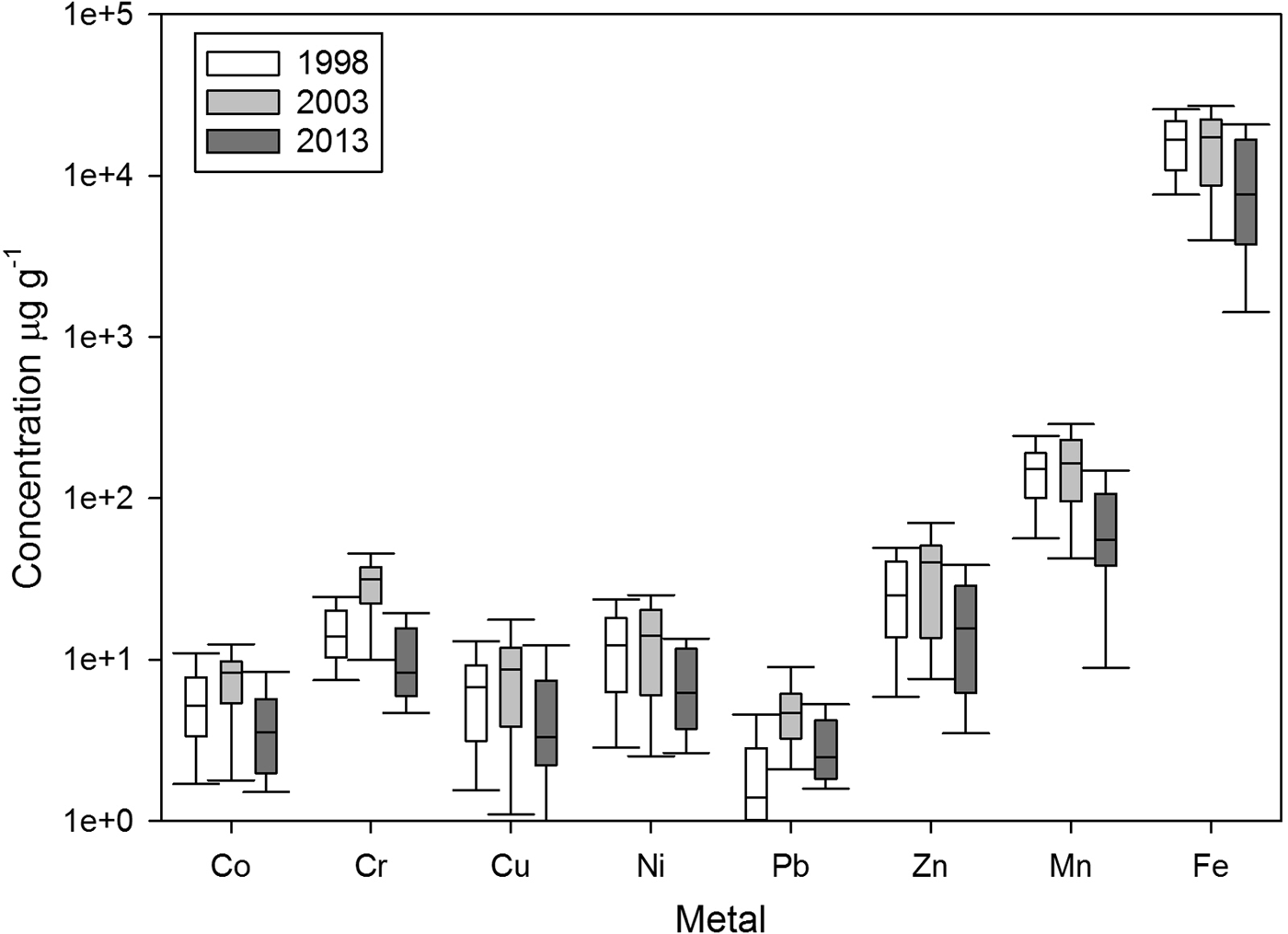
The overall trend for mean trace metal concentration was intermediate in 1998, highest in 2003 and lowest in 2013 (Figure 4). These differences were most apparent in the case of Cr and Pb. On the other hand, Fe showed a decrease over time. However, the concentration of Cr was higher in 2003 than was observed in 1998 and 2013, and the concentration of Pb in 2003 was higher than 1998. Average concentrations for the whole study area across the three sampling years followed the order Pb < Co ~ Cu < Cr ~ Ni < Zn < Mn < Fe.

Fig. 4. Box plots for trace metals concentrations in sediments from the north-western coast of Baja California, Mexico.
Spatio-temporal metals enrichment
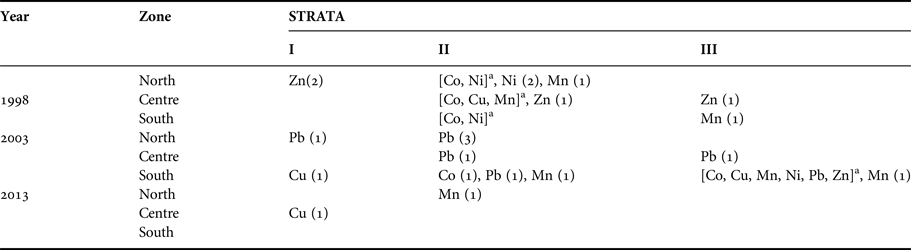
Of the total number of sampling stations, by year, 15% (11 stations) in 1998 and 18% (12 stations) in 2003 were enriched with five metals (Co, Cu, Ni, Zn and Mn) (Table 2), whilst Pb was enriched only in 2003. There was a decrease in the percentage of stations enriched by metals for 2013, with Cu and Mn above enrichment levels in only 2.5% of the stations (two stations). Spatially, trace metal enrichment was found in the sediments of the middle shelf (30–120 m) (Figure 5), whilst for the inner (6–30 m) and outer shelves (120–200 m) a low number of enrichment sites (<2) were present. Only one enriched site was detected for all trace metals, located in the submarine canyon of Bahia de Todos Santos (205 m) south of the area of study.

Fig. 5. Localization of enriched sites for any station with at least one trace metal in this category.
Table 2. Enrichment metals found in sediments. The number of sites enriched is given in parentheses.

a Stations enrichment in more than one metal.
Multivariate analysis
Principal components analysis performed for Bight 98 indicated that environmental variables explained 67.7% of the variability along the first two axes (Table 3). In the first component PC1 (56.4%), the values for most variables were almost equally weighted. The second component PC2 determined that depth, grain size % <63 µm, %OC, Co and Pb accounted for 11.3% of the total variance. The plot showed that stations were arranged along a depth gradient from shallow-intermediate stations (right side of plot) to deep stations (left side of plot) (Figure 6A). In general, stations that showed enrichment had at least one trace metal that was widely dispersed, indicating a high dissimilarity.

Fig. 6. Two-dimensional PCA ordinations on the sedimentary variables for each survey. (A) 1998; (B) 2003; (C) 2013. The north = △, centre = ○ and south = ▽ stations are displayed by depth strata: I (6–30 m); II (31–120 m); III (121–200 m). += site enriched in all trace metals.
Table 3. PCA analysis results.
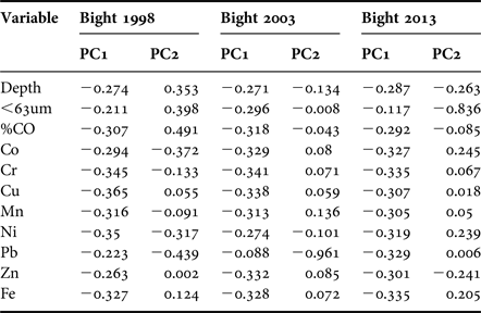
In Bight 2003, environmental variables explained 80.9% of the variability observed in the first two axes (Table 3). The first component PC1 explained 72% of the variability, and the values for most variables were almost equally weighted, with the exception of lead (PC2), which explained 8.9% of the variability. The plot (Figure 6B) showed a better depth gradient relationship than observed in Bight 98. Stations with any trace metal enrichment showed a high similarity, except for three stations (located in the north zone) enriched with lead.
No clear dissimilarity was observed at the station within the centre zone enriched with Cu; however, the middle-depth station from the north zone enriched with Mn was more similar to the deeper stations.
In Bight 2013, 81% of the variability was explained on the first two axes PC1 (71.2%) and PC2 (9.9%) (Table 3). In the first component PC1, the values of most variables were almost equally weighted. The second component PC2 determined that grain size % <63 µm was the most important variable. The plot (Figure 6C) showed that stations were arranged along a depth gradient from shallow-intermediate, to deep stations; however, for 2013, the similarities between shallow stations were higher than observed in middle and deep stations.
General results based on classification and ordination analysis showed that over the three surveys there was an increase in similarity between stations from Bight 1998 to Bight 2013. This indicated more environmental affinity between stations and, therefore, the stratification of stations in shallow, medium and deep zones was clearer for Bight 2013.
Polychaete community structure
SPATIO-TEMPORAL ABUNDANCE AND FAMILY RICHNESS
Analysis of 218 benthic stations sampled from three surveys resulted in a total of 59,373 polychaetes identified in 47 families.
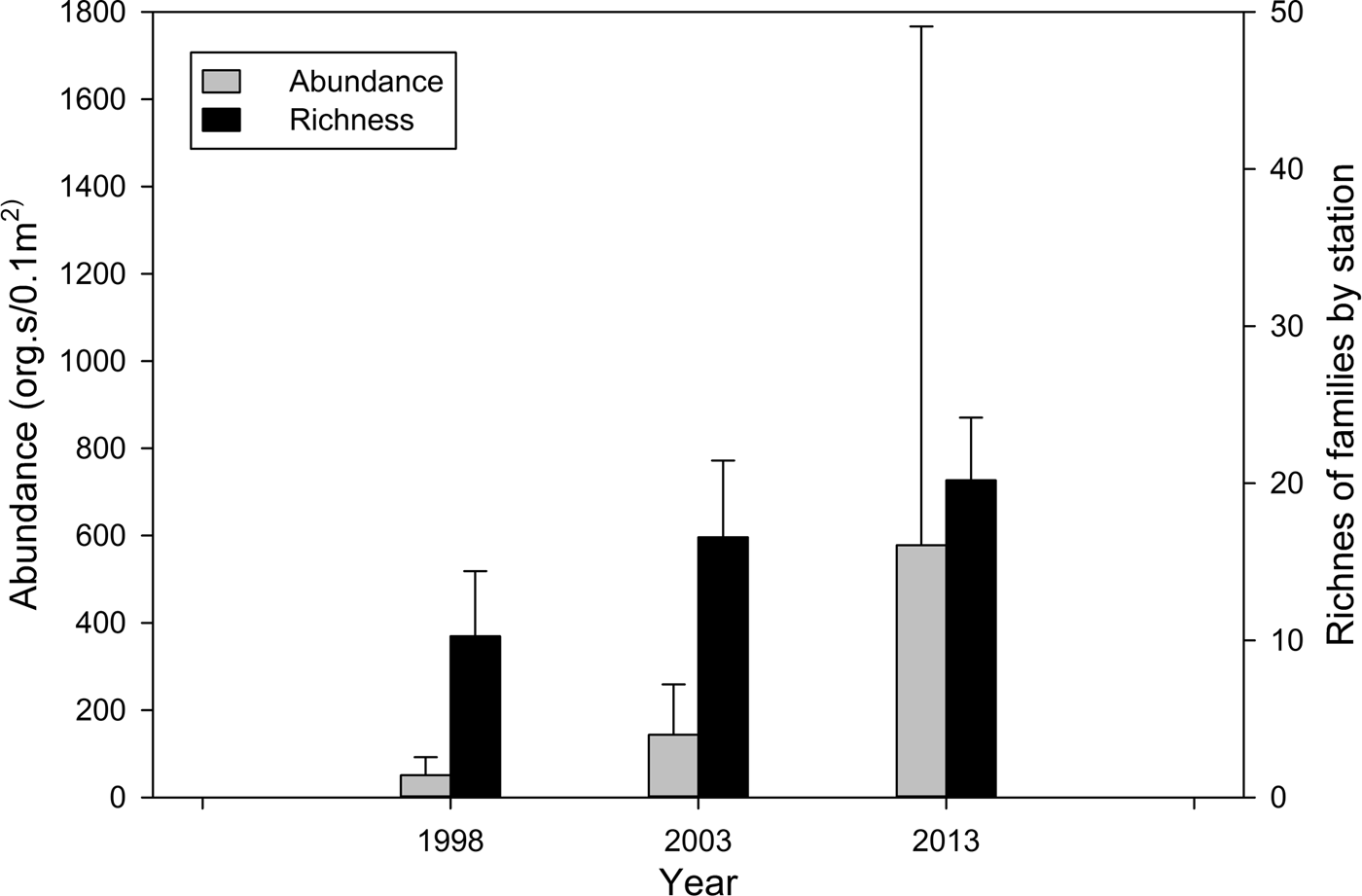
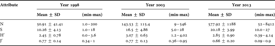
There was a regional and temporal increase in the abundance of polychaetes from 1998 to 2013. The average abundance of polychaetes in the study area increased ~ three times from 1998 to 2003, and for 2013, the abundance increased ~ 10 times with respect to 1998 (Table 4, Figure 7). In 2013, in the north zone, the highest values of abundance for all sampling years were detected, with values between 800 and 8500 ind. 0.1 m−2 (Table 4, Figure 8A).

Fig. 7. Average polychaete abundance and richness (number of families), including SD for the three sampling years.
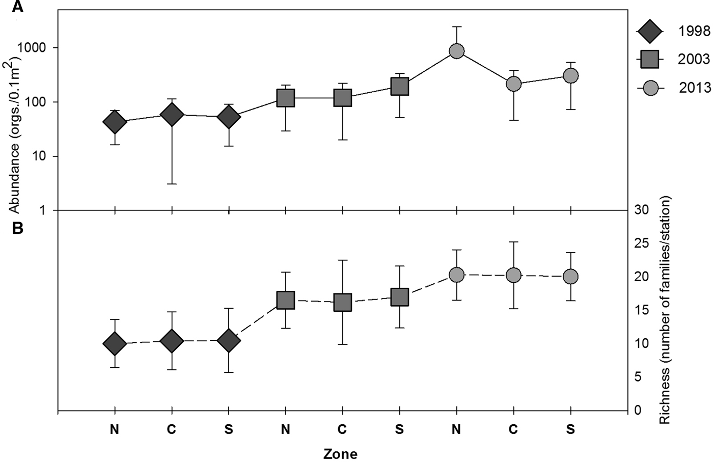
Fig. 8. (A) Average abundance, (B) richness (number of families) of polychaetes within the three zones (north, centre and south) including the SD for the three sampling years.
Table 4. Ecological attributes of benthic Polychaeta fauna in study area. Number of families (S), abundance (N), Evenness's of Pielou (J′) and Shannon-Wiener index (H′).

In the case of family richness, the lowest value in the area was observed in 1998. Family richness in 2003 increased by around 50% with respect to 1998, and for 2013 it doubled with respect to 1998 (Table 4, Figure 8B). Online Appendix A lists the 30 most abundant families, which accounted for 99 and 99.5% of the total abundance of polychaetes in each sampling year, respectively. Most of the 30 families were common among the surveys; however, their frequency increased from 1998 to 2013. Spionidae was the most abundant and frequently observed family, present at 90% of stations, and accounted for ~30% of the total abundance in 1998 and 2003. In 2013, the abundance of spionids was twice that of 1998 (67.4%). Chaetopteridae was neither frequent nor abundant in 1998 and 2003, but in 2013 was the second most abundant family. Phyllodocidae was the fifth most abundant family in 2013, but not abundant in 1998 or 2003.
SPATIO-TEMPORAL POLYCHAETE DIVERSITY
For the area of study, diversity H′ analysis showed an increasing trend from 1998 to 2013 (Table 4). This trend was supported by high values of evenness index between 0.7 and 1. In 1998, similar average values of H′ for the north, centre and south zones were observed (Figure 9A, B). In 2003, decreased values of H′ and J′ for the south zone were observed, whilst, in 2013, the same values decreased for the north zone, where the average diversity was lower in comparison to the rest of the zones.
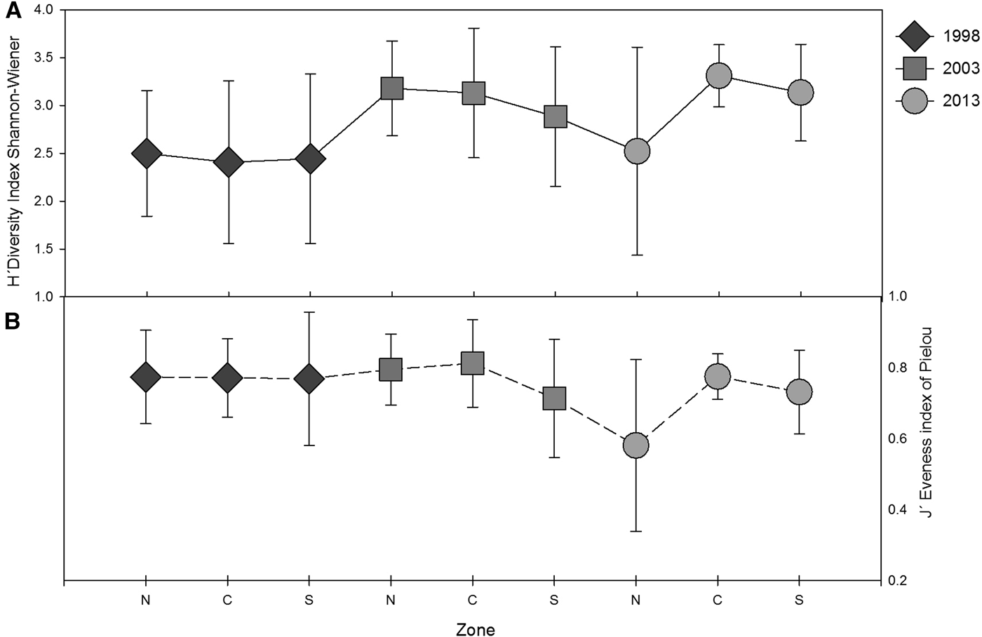
Fig. 9. (A) Shannon–Wiener Diversity index (H′ log2) and (B) evenness index (J′) of the polychaete communities averaged by zone (north, centre and south), including SD for the three sampling years.
The Shannon–Wiener index (H′) suggested in 1998 that 45% of the study area had a moderate ecological and environmental status (Figure 10), while 26.76% had good status, 23.9% had poor status. The remaining 4.2% had bad ecological and environmental status, located near to the discharges from wastewater treatment plants (north zone), the natural discharge of ‘La Misión’ creek (centre zone) and the mouth of Punta Band estuary (south zone).

Fig. 10. Shannon–Wiener (H′ log2) diversity index of polychaete community in relation to ecological quality status in years 1998, 2003 and 2013.
In 2003, the status of the area improved in comparison to 1998 (Figure 10) with the percentage area with moderate ecological and environmental status decreasing to 27.2% of the total area. This was restricted to the areas around the discharge of wastewater treatment plants (north zone), the natural discharge of ‘La Misión’ creek (centre zone) and at the mouth of the Punta Banda estuary (south zone). Good ecological and environmental status increased to 62.1%, and high ecological and environmental status was at 1.5%. While only 9% of the area registered poor ecological and environmental status.
In 2013, the percentage of the area classified as having a bad ecological and environmental status was 7.5% (Figure 10), the highest value of all sampling years around the discharges of wastewater treatment plants (north zone). Small patches of moderate status were observed in the central zone offshore deeper strata, close to a liquefied natural gas plant, in the submarine canyon, Todos Santos Islands and Punta Banda area (south zone).
Multivariate analysis
SPATIAL DISTRIBUTION OF THE FAUNA
Patterns of assemblages were visualized by non-metric multidimensional scaling (nMDS) in two dimensions with a stress value of 0.23 in Bight 1998, 0.21 in Bight 2003 and 0.18 in Bight 2013 (Figure 11A–C) which indicated a good representation of between station similarities that increased over time. nMDS analysis showed differences among sampling years, for Bight 98 sites were widely dispersed; therefore, no clear separation by depth strata or zone was observed (Figure 11A). For Bight 03, deep stations were clearly separated from shallow and middle-depth stations (Figure 11B). In Bight 13, a depth gradient from shallow, to mid and deep stations was observed (Figure 11C).

Fig. 11. Two-dimensional non-metric multidimensional scaling ordination (nMDS) plot on the basis of the Bray–Curtis similarity measure over the density values of polychaete families in each year survey (A–C). The north = △, centre = ○ and south = ▽. Depth strata: I (6–30 m); II (31–120 m); III (121–200 m); nMDS labelled by perturbation status (D–F).
POLYCHAETE ASSEMBLAGES
When stations were labelled according to their status of ecological quality in the previously obtained nMDS for the three surveys, the plots showed an ordination along a gradient of perturbation from high-good to moderate-bad status (Figure 11D–F).
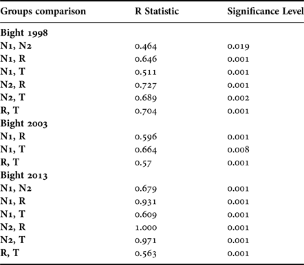
Different similarity thresholds were utilized to determine the main groups in the three surveys; this threshold was low in Bight 1998 (36%), close to 50% in Bight 2003 (48%) and 55.5% in Bight 2013 (Figure 11D–F). The stations with a moderate to high status were grouped at the central part (group of reference conditions ‘R’), stations with good-moderate status were dispersed around the central group (group of transition conditions ‘T’), and bad-moderate status (N1 and N2) widely dispersed around the main central group. Station group N1 grouped mainly stations located close to the discharges of the Tijuana Estuary and the Binational and Punta Bandera wastewater treatment plants located in the north zone. Station group N2 grouped stations mainly located between the wastewater plants from the north zone. The four major groups (R, T, N1 and N2) were determined in Bight 1998 and 2013, but only three major groups (R, T and N1) in Bight 2003 were noted.
SIMPER analysis found the taxa most responsible for the percentage of similarity in Bight 1998 ranged from 42 to 51% (online Appendix B). The Spionidae contributed the most similarity in groups R (28%), T (38%) and N1 (65%), while the Sigalionidae (33%) was the taxa most responsible for the percentage of similarity in group N2. Only four families were associated with 90% of the similarity in group N1, six families in group T, seven in group N2 and 13 families in group R.
SIMPER analysis found the taxa most responsible for the percentage of similarity in Bight 2003 ranged from 51 to 60% (online Appendix B). The Spionidae and Maldanidae contributed the majority of similarity in group R, Spionidae and Cirratulidae contributed most in group T, while in group N1 Glyceridae, Spionidae and Cirratulidae contributed to the majority of similarity. The number of families associated with 90% of the similarity in the groups increased with respect to Bight 1998, nine families in group N1, 11 in group T and 16 families in group R.
SIMPER analysis found the taxa most responsible for the percentage of similarity in Bight 2013 ranged between 62–77% (online Appendix B). In groups R and T, the Spionidae contributed between 15–18% to similarity, while in group N2 the Spionidae contribution was 40, and 56% in group N1, which was the highest contribution. Phyllodocidae and Chaetopteridae contributed the most similarity in groups N1, N2 and T. The Cirratulidae and Maldanidae contributed the most to similarity in group R. The number of families associated with 90% of the similarity in groups increased with respect to previous surveys, nine families in group N1, 14 in group N2, 17 families in group T and 19 families in group R.
Macrofauna community structure was significantly different among the groups in Bight 2013 (ANOSIM, P < 0.001, Table 5). In Bight 1998, stations in group N1 were not significantly different from group N2, and group N2 was not significantly different to group T. All other pairwise comparisons showed significant differences (Table 5). In Bight 2003, only stations in group N1 were not significantly different from group T. These differences suggested that these polychaete assemblages characterized perturbed areas.
Table 5. Anosim analysis results.
ENVIRONMENT–FAUNA RELATIONSHIP
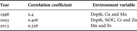
Bio-Env analysis indicated that the environmental variables that best explained changes in polychaete family distribution showed a low correlation. These variables were different in each sampled year; three variables in 1998, four in 2003 and two in 2013 (Table 6). Depth was a common variable for 1998 and 2003, but not in 2013. The variables Cu and Mn were observed in 1998, Cr and Zn in 2003, Mn and Fe in 2013. In 2003, only %CO was present in a combination of variables that best explained changes in polychaete family distribution.
Table 6. Bio-Env analysis results.
SPATIO-TEMPORAL DIFFERENCES
Environment variables
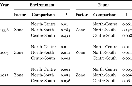
PERMANOVA analysis showed that the set of environmental variables measured in the study area had differences between sampling years, zones and strata (Table 7). Spatial differences showed that the environmental variables in the north zone differed to the centre zone in all three years. In 2003, the centre zone had differed to the south zone.
Table 7. PERMANOVA analysis results.
DISCUSSION
In the study area, the predominance of coarse sediments and the dispersion of pollutants has been previously related to the high energy oceanographic processes of the California Current System (Rodríguez-Villanueva et al., Reference Rodríguez-Villanueva, Martinez-Lara and Macías-Zamora2003; Macías-Zamora et al., Reference Macías-Zamora, Ramírez-Álvarez, Hernández-Guzmán and Mejía-Trejo2016). The observed increase in percentage of silts in the inner shelf (north zone) from 1998 to 2013 could be related with particle discharge from the Binational wastewater treatment plant, which started operations in 1999, discharging 25 million gallons per day of advance primary treatment (http://www.swrcb.ca.gov/sandiego/water_issues/programs/iwtp/index.shtml).
On the other hand, the regional increase in sand fraction detected in 2013 in comparison to previous years could be related to weather characteristics in each sampling year. In 1998, sampling was carried out at the end of the 1997–1998 strong ENSO event, when the annual precipitation was around 500 mm year−1 (Pavía & Badan, Reference Pavía and Badan1998). During this time important inputs of sediment from the coast, wastewater treatment plants, rivers, temporal creeks and non-point sources were introduced to the sea. In 2003 sampling took place after the 2002–2003 weak ENSO event when annual precipitation was ~200 mm year−1 (Alvarez et al., Reference Alvarez, Michel, Reyes-Coca and Troncoso-Gaytan2007). Sampling in 2013 was carried out in severe drought conditions, when the SCB region was in the midst of the worst drought in over a century (Griffin & Anchukaitis, Reference Griffin and Anchukaitis2014).
For coastal zones in southern California, Sabin et al. (Reference Sabin, Jeong, Stolzenbach and Schiff2005) estimated the contribution of trace metals from atmospheric deposition to stormwater was as much as 57–100% of the total trace metal loads in annual stormwater discharges, and further mentioned the importance of this contribution to water bodies near urban centres. In the current study, the lack of this contribution may be related with the decrease in the sediment enrichment of trace metals. Neave et al. (Reference Neave, Glasby, McGuinness, Parry, Streten-Joyce and Gibb2013) observed this effect in their seasonal study, in marine sediments from the northern territory in Australia, where sediments collected during the wet season generally contained the highest metal concentrations, and tended to decrease during the dry season when the sediments generally contained the lowest metal concentrations.
The only site enriched in all trace metals measured was detected in 2003, located at the south zone near the submarine canyon of Todos Santos Bay. This enrichment could be associated with dumping sites of dredged sediments from Ensenada harbour that were in operation during that year. These results were consistent with the enrichment in silver in marine sediments recorded by Gutiérrez-Galindo et al. (Reference Gutiérrez-Galindo, Muñoz-Barbosa, Mandujano-Velasco, Daesslé and Orozco Borbón2010). Romero-Vargas-Márquez (Reference Romero-Vargas Márquez1995) observed high concentrations of several metals, including Cd, Cu, Zn and Ni around the same dumping sites. Lares et al. (Reference Lares, Marinone, Rivera-Duarte, Beck and Sañudo-Wilhelmy2009) registered high concentrations of Zn, Cd and Ni in surface waters around the dumping sites that were attributed to the resuspension and transport of material dumped in this area.
After analysing the spatio-temporal regional changes in the polychaete community structure, higher abundance and diversities were observed than previously reported in the same zone by Rodríguez-Villanueva et al. (Reference Rodríguez-Villanueva, Martinez-Lara and Macías-Zamora2003). The changes through time in abundance and diversity are probably related to regional perturbation caused by the strong ENSO event in 1997–1998, and subsequent weak ENSO event in 2003. In 2013 drought conditions caused less regional perturbation in the benthic environment and therefore favoured a regional increase in abundance and diversity of polychaetes.
The community structure characteristics observed after ENSO events are consistent with those mentioned by Minnich et al. (Reference Minnich, Franco Vizcaíno and Dezzani2000), who determined that two of the main effects of ENSO on invertebrate benthic communities are changes in species composition and alteration in abundance and biomass.
The change in composition in 2013 of Spionidae, and the presence of Chaetopteridae is consistent with that observed by the City of San Diego south bay sampling, where a high dominance of both Spionidae and Chaetopteridae species was reported, as well as an increase in abundance of Spionidae species from 2007–2013. The authors indicated that sediment characteristics and depth primarily controlled the community structure (City of San Diego, 2015). Díaz-Jaramillo et al. (Reference Díaz-Jaramillo, Muñoz, Delgado-Blas and Bertrán2008) observed extensive communities of spionid polychaetes in areas that naturally possess high organic matter, and Elías et al. (Reference Elías, Rivero, Palacios and Vallarino2006) indicated that high densities of spionids are present around sewage outfalls. Therefore, these families could be responding both to local (wastewater treatment plants), regional disturbance effects (drought conditions) as well as oceanographic processes of high energy from the California Current System in the region.
According to Jumars et al. (Reference Jumars, Dorgan and Lindsay2015) the dominant families recorded here are predominately surface deposit feeders (Ampharetidae, Terebellidae and Oweniidae) or subsurface deposit feeders (Maldanidae and Cirratulidae), and only the Onuphidae and Phyllodocidae are considered carnivorous or scavengers.
The Spionidae and almost all benthic Chaetopteridae species use either suspension or surface deposit feeding modes (Jumars et al., Reference Jumars, Dorgan and Lindsay2015). Factors affecting the shift to suspension feeding include the horizontal flux of particles, flow speed and especially suspended food quality (Taghon et al., Reference Taghon, Nowell and Jumars1980; Bock & Miller, Reference Bock and Miller1996). These environmental characteristics may explain the observed changes in community composition for 2013, particularly close to perturbed areas where their abundance was high.
There was only a low spatio-temporal correlation observed between polychaete families and environmental variables, which may be explained by complex and variable ocean current patterns causing sediment heterogeneity (Schiff et al., Reference Schiff, James Allen, Zeng and Bay2000), along with ENSO events and drought condition.
Rodríguez-Villanueva et al. (Reference Rodríguez-Villanueva, Martinez-Lara and Macías-Zamora2003) indicated that depth, sediment grain size and %OC were the environmental variables controlling polychaete diversity in the study area, although these findings may also be a function of current circulation patterns, which dominate this area. In 2003 we found that depth, %OC, Cu and Zn were weakly correlated with polychaete structure.
Muñoz-Barbosa et al. (Reference Muñoz-Barbosa, Gutiérrez-Galindo, Daesslé, Orozco-Borbón and Segovia-Zavala2012) pointed out that Cu and Zn could have an adverse effect on the biota, but the impact and dispersion of chemical characteristics of wastewater plumes from San Diego to Ensenada Bay have been little studied. These plumes can be the primary mechanism for exchange and transfer of nutrients, organic compounds and trace metals to bays and the coastal ocean (Volpe & Esser, Reference Volpe and Esser2002). In our study, the relation of Cu, Cr, Mn and Zinc with the biological pattern in 1998 and 2003 could be related with the regional perturbation by ENSO events that affected the rates of exchange of sediments, nutrients and trace metals in mixed waters into the coastal zone.
Lam & Bishop (Reference Lam and Bishop2008) mentioned that the addition of Fe and Mn from continental margins to the sea, in combination with vertical mixing processes is at least as important as transport of these metals by atmospheric deposition. In 2013, low precipitation and less perturbation by mixing processes resulted in an increasing gradient of Fe and Mn with respect to depth, and conversely these metals were weakly correlated with polychaete structure.
Local effects on benthic community structure were observed and some of these could have resulted from anthropogenic activities within the area. In the north and south zones these effects were closely associated with wastewater treatment plants. In the centre zone the effect from the discharge of the La Misión creek was observed in 1998 and 2003 but not in 2013, probably due to low levels of precipitation. Additionally, effects were seen close to the coast between the centre and south zones near the liquefied natural gas plant. The north zone had differences in both environmental variables and polychaete composition with respect to the centre zone throughout the three sampling years. The exception was in 1998 with no significant differences, possibly because the Binational wastewater treatment plant was not yet in operation.
CONCLUSIONS
From 1998 to 2013 a spatio-temporal benthic analysis was conducted comparing polychaete community structure in the southern end of the Southern California Bight. Environmental variables indicated a change over time in sediment composition with an increase in the sand fraction, a major depth stratification in a gradient from shallow to deep, and a reduction of trace metal enrichment (Co, Cr, Cu, Mn, Ni, Pb and Zn). In 2013 an evident change in polychaete family composition was found with high frequency and abundances of the Spionidae, Chaetopteridae and Phyllodocidae especially close to discharge of wastewater treatment plants (local perturbations). Increased values of abundance, richness and polychaete diversity from 1998 (strong ENSO event) to 2003 (weak ENSO event) and 2013 (drought conditions) may be more directly a function of a decrease of regional perturbations due to oceanographic and weather conditions.
SUPPLEMENTARY MATERIAL
The supplementary material for this article can be found at https://doi.org/10.1017/S0025315417000637.
ACKNOWLEDGEMENTS
We would like to thank Algalita Marine Research Foundation for providing ship support and Captain Charles Moore for logistics in sampling, transport and assistance. Finally, we would also like to thank Ricardo Martinez-Lara for valuable comments on an earlier version of this manuscript.
FINANCIAL SUPPORT
The Autonomous University of Baja California partially financed this work with the internal project from 17th call contract #_629. Thanks are also given to CONACyT for providing a doctoral scholarship to Arturo Alvarez-Aguilar.