INTRODUCTION
As a primary producer, diatoms play an important role in the functioning of microbial food webs and geo-chemical cycles of silica and carbon in aquatic ecosystems (Round et al., Reference Round, Crawford and Mann1990; Berger & Wefer, Reference Berger and Wefer1991; Finkelstein & Davis, Reference Finkelstein and Davis2006; Smucker & Vis, Reference Smucker and Vis2011a, Reference Smucker and Visb; Di et al., Reference Di, Liu, Wang, Dong, Li and Shi2013; Liu et al., Reference Liu, Zhang and Xu2013, Reference Liu, Zhang and Xu2014). With their short cycle development, high species diversity, a wide range of occurrence, and sensitivity to environmental changes, they are particularly useful to indicate the intensity of anthropogenic impact and climate change in most aquatic ecosystems compared with the other living organisms (e.g. macroinvertebrates, molluscs, fish) (Round et al., Reference Round, Crawford and Mann1990; Zielinski & Gersonde, Reference Zielinski and Gersonde1997; Wan Mazahn & Mansor, Reference Wan Mazanh and Mansor2002; Duong et al., Reference Duong, Coste, Feurtet-Mazel, Dang, Gold, Park and Boudou2006; Berthon et al., Reference Berthon, Bouchez and Rimet2011; Stenger-Kovács et al., Reference Stenger-Kovács, Lengyel, Crossetti, Üveges and Padisák2013; Chen et al., Reference Chen, Qin, Stevenson and McGowan2014).
Jiaozhou Bay is a large eutrophic basin, covering an area of about 390 km2 with an average depth of about 7 m. It is connected to the Yellow Sea via a narrow mouth about 2.5 km in width, surrounded by Qingdao, northern China (Shen, Reference Shen2001; Liu et al., Reference Liu, Wei, Liu and Zhang2004; Xu et al., Reference Xu, Jiang, Al-Rasheid, Al-Farraj and Song2011). So far, Jiaozhou Bay has been stressed by human activities and is thus subject to eutrophication events (Jiang et al., Reference Jiang, Xu, Hu, Zhu, Al-Rasheid and Warren2011, Reference Jiang, Zhu, Zhang, Al-Rasheid and Xu2013, Reference Jiang, Xu and Warren2014). Although several studies have been conducted on community research of plankton in Jiaozhou Bay (Nuccio et al., Reference Nuccio, Melillo, Massi and Innamorati2003; Liu et al., Reference Liu, Zhang, Chen and Zhang2005, Reference Liu, Sun, Zhang and Liu2008, Reference Liu, Zhang and Xu2014), the annual cycle of planktonic diatoms has yet to be investigated.
In this study, a 1-year baseline survey on annual dynamics in community patterns of planktonic diatoms was performed during the period of June 2007–May 2008 in Jiaozhou Bay. Our aims of this study were: (1) to investigate the temporal variations in species composition, distribution and community patterns of planktonic diatoms; and (2) to determine the environmental drivers for seasonal shift in the diatom community structure in the marine ecosystem.
MATERIALS AND METHODS
Sampling stations and data collection
Five sampling sites (A–E) were selected in Jiaozhou Bay (35°55′–36°18′N 120°04′–120°23′E), surrounded by Qingdao, northern China (Figure 1). A total of 24 cruises were performed biweekly over a 1-year period from June 2007 to May 2008.

Fig. 1. Sampling stations of planktonic ciliates in Jiaozhou Bay.
Water samples were collected at a depth of about 1 m. Both for quantitative measures and for species identification of diatoms, 1000 mL of seawater was fixed with acid Lugol's iodine solution (2% final concentration, volume/volume) (Jiang et al., Reference Jiang, Xu, Hu, Zhu, Al-Rasheid and Warren2011).
Water temperature (T), pH, salinity (Sal) were measured in situ, using a multi-parameter kit (MS5, HACH). Soluble reactive phosphate (SRP), ammonium nitrogen (NH4-N), nitrate nitrogen (NO3-N) and nitrite nitrogen (NO2-N) were determined using a UV-visible spectrophotometer (DR-5000, HACH) according to the ‘Standard Methods for the Examination of Water and Wastewater’ (APHA, 1992).
Identification and enumeration
For purposes of identification and enumeration, 1000 mL of Lugol's–fixed seawater was settled for 48 h resulting in 30 mL of concentrated sediment (Utermöhl, Reference Utermöhl1958). A 0.1 mL aliquot of each concentrated sample was placed in a Perspex chamber and the diatoms were counted under a light microscope at magnification 400× (Xu et al., Reference Xu, Song, Warren, Al-Rasheid, Al-Farraj, Gong and Hu2008). Five aliquots from each sample were counted and yielded a standard error (SE) of <8% of the mean values of counts (Xu et al., Reference Xu, Song, Warren, Al-Rasheid, Al-Farraj, Gong and Hu2008). Diatom identification and enumeration were carried out following the methods outlined by Round et al. (Reference Round, Crawford and Mann1990). The taxonomic classification of diatoms was based on the published references to keys and guides such as Hasle & Syvertsen (Reference Hasle, Syvertsen and Tomas1997). The taxonomic scheme used was according to Round et al. (Reference Round, Crawford and Mann1990).
Data analyses
Species diversity (Shannon diversity) (H′), evenness (Pielou's evenness) (J′) and richness (Marglef's richness) (D) of samplings were calculated as follows:
 $$H^{\prime} = \sum\limits_{i = {\rm 1}}^S {Pi{\rm (ln}Pi{\rm )}} $$
 $$J^{\prime} = H^{\prime}/{\rm ln(}S{\rm )}$$
 $$D = (S - {\rm 1})/{\rm ln(}N{\rm )}$$
where Pi = proportion of the total count arising from the ith species; S = total number of species; and N = total number of individuals (Xu et al., Reference Xu, Song, Warren, Al-Rasheid, Al-Farraj, Gong and Hu2008).
Multivariate analyses of temporal variations in planktonic diatom communities were performed using the PRIMER v6.1.16 package (Clarke & Gorley, Reference Clarke and Gorley2006) and the PERMANOVA+ for PRIMER (Anderson et al., Reference Anderson, Gorley and Clarke2008). The seasonal species distributions of the diatoms were summarized using clustering submodule, while the seasonal shift in community patterns was summarized using canonical analysis of principal coordinates (CAP). Differences in species distribution patterns among groups were signified by the submodule ANOSIM, while those in community pattern between seasons of samples were tested by the submodule PERMANOVA (Anderson et al., Reference Anderson, Gorley and Clarke2008). The significance of biota-environment correlations was tested using Mental (RELATE) analysis, while the top 10 significant correlations between biotic and abiotic matrices were explored using the submodule BIOENV (biota-environment) (Clarke & Gorley, Reference Clarke and Gorley2006). Bray–Curtis similarity matrix for biotic data was computed from square root transformed species-abundance data, while Euclidean distance matrix for abiotic data was calculated from log-transformed environmental variable data (Xu et al., Reference Xu, Jiang, Al-Rasheid, Al-Farraj and Song2011). It should be noted that, to obtain the similarity matrix for clustering analysis of species distributions, the species abundance data were standardized before data transformation (Xu et al., Reference Xu, Song, Warren, Al-Rasheid, Al-Farraj, Gong and Hu2008).
Univariate analyses of correlations were carried out using the statistical program SPSS v16.0. Data were log-transformed before analyses (Xu et al., Reference Xu, Song, Warren, Al-Rasheid, Al-Farraj, Gong and Hu2008).
RESULTS
Environmental parameters
The mean values of 11 environmental variables for each month are summarized in Table 1. Water temperature followed a clear seasonal pattern, ranging from 1.4 to 27.5°C (mean 14.7°C). Salinity was around 30.0 psu and levelled at a stable level over the 1-year cycle, except sharp drops in late August (21.3 psu) and in late September (20.4 psu). The pH values ranged from 7.8 to 8.6, averaging 8.2. SRP ranged from 0.1 to 0.4 mg L−1 (mean value of 0.2 mg L−1) with a minor peak in early August. The mean concentration of NH4-N and NO3-N peaked in late September, whereas low concentrations of NO2-N were maintained throughout the year apart from a minor increase between July and September.
Table 1. Average values of environmental variables monitored within each month in Jiaozhou Bay during the 1-year cycle of June 2007–May 2008.

Sal: salinity; NH4-N: ammonium nitrogen; NO3-N: nitrate nitrogen; NO2-N: nitrite nitrogen; SRP: soluble active phosphate.
Species composition and seasonal distribution
The species composition of diatom communities recorded during the study period is summarized in Table S1. A total of 75 diatom species, representing 40 genera, 28 families, 19 orders and three classes, were identified during the 1-year survey. Of these species, 11 forms were distributed in all seasons, while 27, 35, 56 and 28 taxa only occurred in spring, summer, autumn and winter, respectively.
The clustering analysis resulted in 75 diatom species falling into four groups with a similar distribution pattern for each at a 49% similarity level (Figure 2a). For example, group I comprised 15 species, mainly dominated in late winter and early spring (Figure 2a: I); group II comprised 27 species which predominated in late spring and early summer (Figure 2a: II); group III comprised 28 taxa, which mainly dominated in late summer and early autumn (Figure 2a: III); and group IV included only five species with high occurrence in late autumn and early winter (Figure 2a: IV). Analysis of similarities (ANOSIM) signified the differences among the four groups (Global R = 0.894, P < 0.001), and between each pair of the groups (P < 0.001).
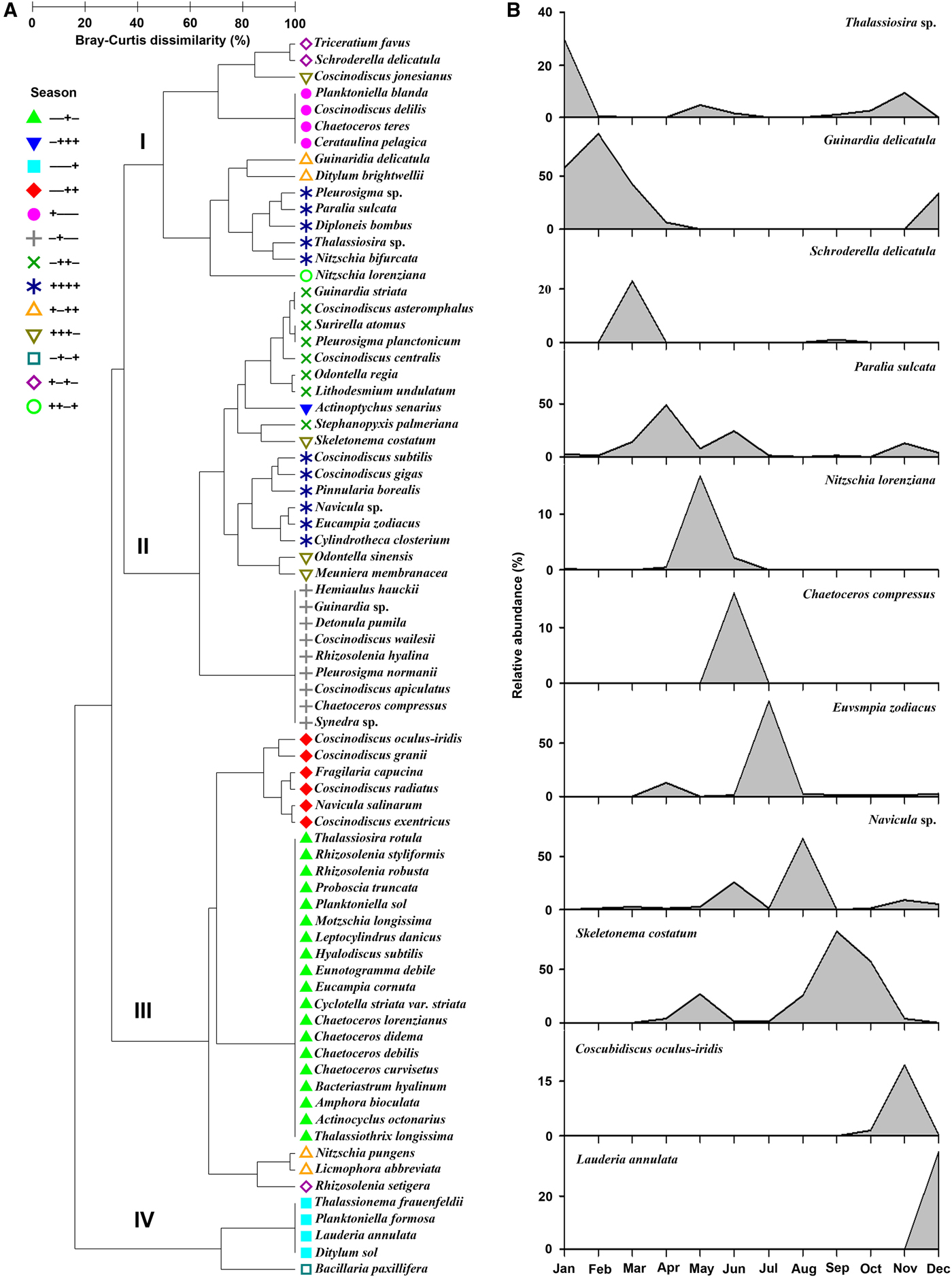
Fig. 2. Seasonal variation in species composition of planktonic diatoms (A), and the temporal succession of 11 dominant species during a 1-year cycle (B). I–IV = group I–IV.

Fig. 3. Annual variations in species number (A), abundance (B, cells L−1), relative species number (C) and relative abundance (D) of the diatoms in Jiaozhou Bay during the study period. Others = sum of Chaetocerotales, Lithodesmiales, Triceratlales, Anaulales, Licmophorales, Thalassionematales, Fragilariales, Surireliales, Thalassiophysales and Melosirales.
A total of 11 dominant species were identified, with a contribution of more than 15% of the total diatom abundance in a month for each (Figure 2b). Five of these species (Paralia sulcata, Nitzschia lorenziana, Schroderella delicaula, Guinarlia delicatula and Thalassiosira sp.) peaked mainly in the late winter and early spring season, four (Chaetoceros compressus, Euvsmpia zodiacus, Skeletonema costatum and Navicula sp.) dominated the samples in late summer and early autumn, and the other two (Coscubidiscus oculus-iridis and Lauderia annuluata) occurred in late autumn and early winter (Figure 2b).
Annual variation in species number, abundance and biomass
The annual variations in species number showed a unimodal distribution peaking in September (Figure 3a). Parallales, Naviculales, Hemiaulales, Coscinodicales, Rhizosoleniales and Thalassiosirales were primarily responsible for taxonomic composition.
The diatom abundances also peaked in unimodal model with maximum value (7.46 × 10⁴ cells L−1) in autumn (Figure 3b). Hemiaulales, Naviculales and Thalassiosirales were the primary contributors to the communities (Figure 3b).
Seasonal variation in community pattern
Although the orders Parallales, Naviculales, Hemiaulales, Coscinodicales, Rhizosoleniales and Thalassiosirales occurred in almost all months, the community patterns showed a clear seasonal variation, especially in the relative abundances (Figure 3c, d). For example, Rhizosoleniales, Parallales and Naviculales dominated the samples in spring (March to May), followed by dominant taxa Hemiaulales and Niviculales in summer (June to August); and Thalassiosirales and Coscinodiscales predominated the samples in autumn (September to November), followed by the dominant Rhizosoleniales in winter (December to February) (Figure 3d).
By canonical analysis of principal coordinates (CAP), the 120 data points showed a clear seasonal shift: the first axis (CAP 1) separated the samples in summer and autumn (on the right) from those in winter and spring (on the left), while data points in summer (upper) and those in autumn (lower) were discriminated by the second axis (CAP 2) (Figure 4a). PERMANOVA test revealed a significant difference between each pair of seasonal group (P < 0.05), except the pair of spring and winter (P = 0.06).

Fig. 4. Canonical analysis of principal coordinates (CAP) on seasonal scale for 120 data points of the diatom communities in Jiaozhou Bay during the study period (top), and correlations of 11 dominant species with the two CAP axes (below).
Vector overlay of Pearson correlations of the 11 dominant species with the canonical analysis of principal coordinates (CAP) axes was also shown in Figure 4b. Of these, three species (Eucampia zodiacus, Chaetoceros compressus and Navicula sp.) pointed toward the sample cloud of (upper right), three (Skeletonema costutum, Coscinodiscus oculus-iridis and Thalassiosira sp.) toward that of autumn (lower right), and the other five (e.g. Nitzshia lorenziana, Guinardia delicatula and Paralia sulcata) toward the data points in spring and winter (Figure 4b).
Annual variation in diversity measures
The annual variation in species diversity (H′), evenness (J′) and richness (D) indices in 12 months is shown in Figure 5. All three community parameters showed a similar temporal variation with two peaks in spring and autumn, respectively (Figure 5).

Fig. 5. Annual variations in species richness (a), evenness (b) and diversity (c) of the diatom communities in Jiaozhou Bay during the study period.
Interaction between biotic data and environmental variables
Canonical analysis of principal coordinates (CAP) showed that the environmental conditions represented a clear seasonal shift (Figure 6). Mental analysis revealed a significant correlation between annual variation in community pattern and changes of environmental variables (R = 0.157; P < 0.05). Biota-environment (BIOENV) analysis showed that the seasonal shift in community pattern was shaped by environmental drivers, especially temperature, pH, salinity and nutrients (NO3-N, NO2-N, SRP), alone or in combination (Table 2).
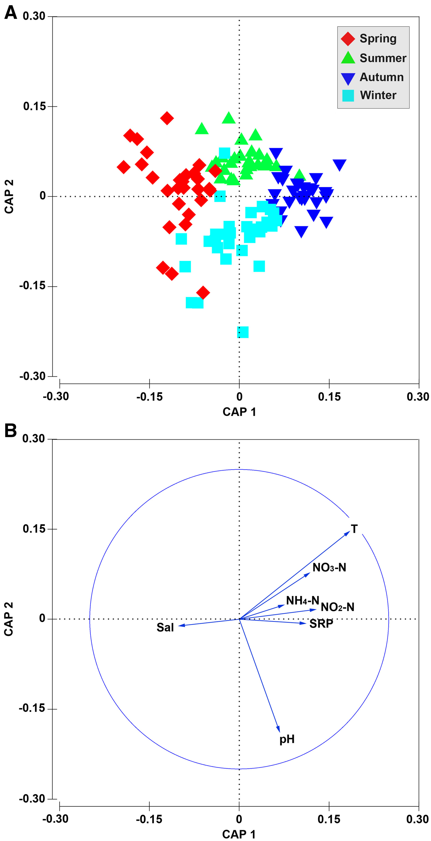
Fig. 6. Canonical analysis of principal coordinates (CAP) on seasonal scale for 120 data points of the environmental variables in Jiaozhou Bay during the study period (A), and correlations of environmental variables with the two CAP axes (B).
Table 2. Summary of results from biota-environment (BIOENV) analysis showing the 10 best matches of environmental variables with temporal variation in community patterns in coastal waters of the Yellow Sea during the study period.

ρ = Spearman correlation coefficient. Sal = salinity; SRP = soluble active phosphate; NO3-N: nitrate nitrogen; NO2-N: nitrite nitrogen.
Of 11 dominant species, four (Paralia sulcata, Skeletonema costatum, Guinardia delicatula and Nitzschia lorenziana) were significantly related with temperature, pH and/or nutrients (Table 3).
Table 3. Summary of results from correlation analyses between 11 four dominant diatom species and environmental variables in coastal waters of the Yellow Sea during the study period.

Sal = salinity; SRP = soluble active phosphate; NO3-N: nitrate nitrogen; NO2-N: nitrite nitrogen. *Significant difference at P < 0.05.
DISCUSSION
In this study, a total of 75 diatom species were identified during one annual cycle in Jiaozhou Bay. The annual variations in both species number and abundance showed a similar pattern, i.e. peaked during the period of July–September. Compared with the Liu et al. (Reference Liu, Sun, Chen and Zhang2003a, Reference Liu, Sun and Zhangb) reports in summer (August), using a trawling method, the species number and abundance in the same month were low (21 vs 34; 6.4 × 10⁴ vs 1.07 × 10⁵ cells L−1).
So far, although there have been a few reports on community research of diatoms, little information could be reported on the annual variation or seasonal shift in planktonic diatom community structure and their environmental drivers in Jiaozhou Bay (Liu et al., Reference Liu, Sun, Chen and Zhang2003a, Reference Liu, Sun and Zhangb, Reference Liu, Sun, Zhang and Liu2008). Our data revealed that planktonic diatom assemblages represented a clear annual/seasonal variation in terms of community structure. For example, of 75 diatom species, 27, 35, 56 and 28 occurred in spring, summer, autumn and winter, with 11 dominant species predominating the samples in different seasons. Furthermore, canonical analysis of principal coordinates (CAP) and PERMANOVA test demonstrated a significant seasonal shift in the community pattern, each of which had its own most contributive species.
Mental (RELATE) analysis revealed that the temporal variation in the diatom community structure was significantly correlated with changes of environmental variables, especially the combination of water temperature, pH and nutrients. Pearson correlation analysis demonstrated that a total of four dominant/common species were significantly correlated with temperature, pH and/or nutrient variables. These results imply that the seasonal shift in planktonic diatom community structure is significantly shaped by environmental drivers, especially the water temperature and nutrients.
In addition, the biodiversity measures (i.e. species diversity, evenness and richness indices) represented a similar seasonal variation, generally peaking in spring and autumn seasons in our study. However, it should be noted that these biological indices failed to show significant correlations with environmental parameters. This is consistent with the previous report (e.g. Xu et al., Reference Xu, Song, Warren, Al-Rasheid, Al-Farraj, Gong and Hu2008).
In summary, the diatom assemblages showed a clear seasonal shift in both species distribution and community structure, and the water temperature, pH and nutrients were the main environmental drivers in the eutrophic basin ecosystem. Further studies, however, are necessary in a range of seas and over long-term periods in order to verify these conclusions.
Supplementary material
To view supplementary material for this article, please visit http://dx.doi.org/ 10.1017/S0025315415000673.
ACKNOWLEDGEMENTS
Our special thanks are due to: Dr Xinpeng Fan, Dr Jiamei Jiang and Dr Xumiao Chen, Laboratory of Protozoology, Institute of Evolution and Marine Biodiversity, Ocean University of China, China, for their help in sampling and enumeration.
FINANCIAL SUPPORT
This work was supported by the Darwin Initiative Programme (Project No. 14-015) which is funded by the UK Department for Environment, food and Rural Affairs.