


INTRODUCTION
The marine environment off the coast of southern Africa is one of the most diverse, complex and highly variable in the world (Lutjeharms et al., Reference Lutjeharms, Monteiro, Tyson and Obura2001). The distribution of the Cape Hope squid Loligo reynaudii (locally known as chokka) along this coastline is largely influenced by the warm Angola current and the cold Benguela current upwelling system along the West African coast and the warm Agulhas current system along the south-east coast (Figure 1). Loligo reynaudii inhabits these three different environments (south coast of South Africa, west coast of South Africa, and southern Angola) with an apparent break in its distribution off the coast of Namibia (Shaw et al., Reference Shaw, Hendrickson, McKeown, Stonier, Naud and Sauer2010). In South Africa, two-thirds of the adult biomass is concentrated on the eastern Agulhas Bank shelf where it has become an important fishery resource, targeted by a major commercial hand-line jig fishery (6000–13,000 t caught annually) since the mid-1980s (Augustyn, Reference Augustyn1989, Reference Augustyn1991; Augustyn et al., Reference Augustyn, Roel, Cochrane, Okutani, O'Dor and Kubodera1993, Arkhipkin et al., Reference Arkhipkin, Rodhouse, Pierce, Sauer, Sakai, Allcock, Arguelles, Bower, Castillo, Ceriola, Chen, Chen, Diaz-Santana, Downey, Gonzales, Granados Amores, Green, Guerra, Hendrickson, Ibáñez, Ito, Jereb, Kato, Katugin, Kawano, Kidokoro, Kulik, Laptikhovsky, Lipinski, Liu, Mariátegui, Marin, Medina, Miki, Miyahara, Moltschaniwskyj, Moustahfid, Abhitabhata, Nanjo, Nigmatullin, Ohtani, Pecl, Perez, Piatkowski, Saikliang, Salinas–Zavala, Steer, Tian, Ueta, Vijai, Wakabay Ashi, Yamaguchi, Yamashiro, Yamashita and Zeidberg2015). In addition, 200–500 t is caught annually as a by-catch in the demersal trawl fisheries (Augustyn & Roel, Reference Augustyn and Roel1998; Arkhipkin et al., Reference Arkhipkin, Rodhouse, Pierce, Sauer, Sakai, Allcock, Arguelles, Bower, Castillo, Ceriola, Chen, Chen, Diaz-Santana, Downey, Gonzales, Granados Amores, Green, Guerra, Hendrickson, Ibáñez, Ito, Jereb, Kato, Katugin, Kawano, Kidokoro, Kulik, Laptikhovsky, Lipinski, Liu, Mariátegui, Marin, Medina, Miki, Miyahara, Moltschaniwskyj, Moustahfid, Abhitabhata, Nanjo, Nigmatullin, Ohtani, Pecl, Perez, Piatkowski, Saikliang, Salinas–Zavala, Steer, Tian, Ueta, Vijai, Wakabay Ashi, Yamaguchi, Yamashiro, Yamashita and Zeidberg2015). In southern Angola artisanal fishers catch L. reynaudii close to shore from rafts, using homemade jigs and hand-lines (Sauer et al., Reference Sauer, Downey, Lipinski, Roberts, Smale, Glazer, Melo, Rosa, Pierce and O'Dor2013).

Fig. 1. The current known distribution of Loligo reynaudii, with major oceanographic features of the different regions indicated (modified from Henriques et al., Reference Henriques, Potts, Sauer and Shaw2012). Morphological and genetic sampling locations of Loligo reynaudii on the south and west coast of Southern Africa are shown. PN, Port Nolloth; YZ, Yzerfontein; CT, Cape Town; CA, Cape Agulhas; MB, Mossel Bay; PB, Plettenberg Bay; SF, Cape St Francis; PE, Port Elizabeth; PA, Port Alfred.
Although a number of studies into the stock structure of L. reynaudii have been attempted in the last decade (using various biological and genetic techniques, e.g. Olyott, Reference Olyott2002; Olyott et al., Reference Olyott, Sauer and Booth2006, Reference Olyott, Sauer and Booth2007; Shaw et al., Reference Shaw, Hendrickson, McKeown, Stonier, Naud and Sauer2010; Stonier, Reference Stonier2012), its demography still remains unclear. Due to lengthy planktonic paralarval stages (40-day passive period) with the potential for high dispersal rates (Roberts & Mullon, Reference Roberts and Mullon2010), highly migratory adult stages (Sauer, Reference Sauer1995; Sauer et al., Reference Sauer, Lipinski and Augustyn2000) and a lack of obvious physical geographic barriers to movement along the coastline, genetic homogeneity of the South African stock was previously assumed. This assumption was questioned by Olyott et al. (Reference Olyott, Sauer and Booth2007), who suggested that juveniles growing under different environmental conditions on the western Agulhas Bank could result in discrete subpopulations with different biological characteristics such as slower growth rates and larger size at maturity. The influence of water temperature on the growth of other cephalopod species is well known (Forsythe et al., Reference Forsythe, Derusha and Hanlon1994; Carvalho & Nigmatullin, Reference Carvalho, Nigmatullin, Rodhouse, Dawe and O'Dor1998; Forsythe, Reference Forsythe2004).
A subsequent molecular study by Shaw et al. (Reference Shaw, Hendrickson, McKeown, Stonier, Naud and Sauer2010) indicated small but statistically significant genetic differences among some L. reynaudii samples, suggesting a more complicated stock structure. Although no significant differences were found between genetic samples of different spawning aggregations across the main spawning range on the eastern Agulhas Bank, subtle differences were found in geographically more distant samples from the western Agulhas Bank (Shaw et al., Reference Shaw, Hendrickson, McKeown, Stonier, Naud and Sauer2010). Such differences may necessitate a rethink of the current management strategy. A finer scale study of this region was therefore suggested to further investigate the possibility of geographically fragmented stocks and stock boundaries.
Although studying geographic variation has been an accepted method in fish stock discrimination for over a century (Ihssen et al., Reference Ihssen, Booke, Casselman, McGlade, Payne and Utter1981), and has been extended to cephalopods such as octopods (Voight, Reference Voight2002; Lefkaditou & Bekas, Reference Lefkaditou and Bekas2004) and sepiids (Guerra et al., Reference Guerra, Perez-Losada, Rocha and Sanjuan2001; Kassahn et al., Reference Kassahn, Donnellan, Fowler, Hall, Adams and Shaw2003; Neige, Reference Neige2006), the use of morphometric data has not yet been attempted for L. reynaudii. Morphometric studies have been widely used to distinguish between species of squid (Haefner, Reference Haefner1964; Lipinski, Reference Lipinski1981; Augustyn & Grant, Reference Augustyn and Grant1988; Pierce et al., Reference Pierce, Hastie, Guerra, Thorpe, Howard and Boyle1994a; Sanchez et al., Reference Sanchez, Perry and Trigg1996; Bonnaud et al., Reference Bonnaud, Rodhouse and Boucher-Rodoni1998; Pineda et al., Reference Pineda, Hernandez, Brunetti and Jerez2002) and to study the geographic variation of population units and fishery stocks within species of squid (Kashiwada & Recksiek, Reference Kashiwada and Recksiek1978; Kristensen, Reference Kristensen1982; Brunetti & Ivanovic, Reference Brunetti and Ivanovic1991; Boyle & Ngoile, Reference Boyle, Ngoile, Okutani, O'Dor and Kubodera1993; Pierce et al., Reference Pierce, Thorpe, Hastie, Brierly, Guerra, Boyle, Jamieson and Avila1994b; Borges, Reference Borges1995; Zecchini et al., Reference Zecchini, Vecchione and Roper1996; Carvalho & Nigmatullin, Reference Carvalho, Nigmatullin, Rodhouse, Dawe and O'Dor1998; Hernandez-Garcia & Castro, Reference Hernandez-Garcia and Castro1998; Vega et al., Reference Vega, Rocha, Guerra and Osorio2002; Liao et al., Reference Liao, Liu and Hung2010). It is important to note, however, that unlike molecular markers, phenotypic variation in body parts is markedly influenced by environmental factors (Carvalho & Nigmatullin, Reference Carvalho, Nigmatullin, Rodhouse, Dawe and O'Dor1998) and does not always result from genetic divergence (Cadrin, Reference Cadrin2000). Therefore, phenotypic variation may only provide indirect indication of stock structure (Begg et al., Reference Begg, Friedland and Pearce1999). Although they do not provide direct evidence of genetic isolation between stocks, they can indicate separation of post-larval stocks living in different environmental regimes (Begg et al., Reference Begg, Friedland and Pearce1999). Phenotypic markers may therefore be more useful for studying short-term, environmentally induced variation, as opposed to long-term genetic variation.
In an attempt to better understand the stock structure of L. reynaudii in South African waters this study undertook morphometric analysis across the distributional range of the species, and a more geographically concentrated genetic study of samples from across the Agulhas Bank region.
MATERIALS AND METHODS
Collection of samples
Loligo reynaudii samples from South Africa were collected utilizing various commercial jig vessels and a demersal trawl research vessel (Figure 1). The south coast demersal research survey (8 April 2011–13 May 2011) covered the shelf between 20°E (Cape Agulhas) and 27°E (Port Alfred) and the west coast survey (9 January 2012–13 February 2012) between 20°E (Cape Agulhas) and 29°S (Orange River). These demersal surveys provided for the collection of random samples over a range of shallow and deep areas on the south and west coast of South Africa. Between June and November 2011 additional samples were collected on board various commercial jig vessels fishing in the main inshore spawning areas which were not covered during the south coast demersal trawl survey. Samples caught by the artisanal jig fishery in southern Angola (in the coastal waters between 15° and 17°S) were collected from a single hawker at a fish market in Namibe, the species’ northern-most known geographic limit (Roberts et al., Reference Roberts, Downey and Sauer2012). Only adult squid were sampled, ranging in length from 180–420 mm dorsal mantle length (DML) for males and 150–260 mm DML for females.
All squid were frozen and transported to Rhodes University, South Africa, where they were kept at −20 °C until analysis. Genetic material in the form of tentacle clippings was collected from subsamples of squid caught in the Agulhas Bank and West Coast regions. The clippings were taken immediately after capture and stored in 70% ethanol until processed.
Selection of individuals
A total of 544 male and 535 female individuals from the three regions were used in the classification analyses. The average DML length of males (279.3 mm Angola, 299.8 mm south coast, 250.6 mm west coast) and females (185.8 mm Angola, 207.4 mm south coast, 190.8 mm west coast) from each region differed only slightly (see online Appendix A for the descriptive statistics of all character measurements taken). For both males and females the south coast subsample size was by far the largest.
All samples used in the classification analysis were classified as adults with maturity stages of 3 (preparatory), 4 (maturing) and 5 (mature), according to Lipinski's universal maturity scale for commercially important squid (Lipinski, Reference Lipinski1979; Lipinski & Underhill, Reference Lipinski and Underhill1995). No samples were classified as belonging to stages 1 (juvenile) and 2 (immature).
Morphometric measurements
Forty-three morphometric characters (Table 1) of the soft body parts (body, head, arms, tentacles) and hard structures (gladius, sucker rings, lower beak, statolith) were measured from each sample. Beak morphometric characteristics were modified from Clarke (Reference Clarke1986), statolith morphometric characters from Clarke & Maddock (Reference Clarke, Maddock, Clarke and Trueman1988) and gladius, sucker rings and soft parts were selected and modified from Lipinski (Reference Lipinski1981). Detailed specifics on the measurements taken for each soft part and hard structure can be seen in Table 1 and Figures 2–4. In order to prevent any warping of morphological characteristics, which can happen with repeated freezing and thawing (Lipinski, Reference Lipinski1981), each specimen was defrosted only once at room temperature before morphometric measurements were taken. No measurements were made on soft parts or hard structures which appeared to be damaged or to have suffered previous damage (e.g. missing arm and tentacle tips; re-grown arms and tentacles; damaged gladius, lower beaks, sucker rings and statoliths). All morphometric measurements were made by the senior author and under standardized conditions to avoid unnecessary variation in measurements.

Fig. 2. Soft part morphometric measurements recorded for Loligo reynaudii in this study, based on the work by Lipinski (Reference Lipinski1981). (A) soft part dimensions (taken from Pierce et al., Reference Pierce, Thorpe, Hastie, Brierly, Guerra, Boyle, Jamieson and Avila1994b), (B) fin angle dimension (taken from Pierce et al., Reference Pierce, Thorpe, Hastie, Brierly, Guerra, Boyle, Jamieson and Avila1994b).
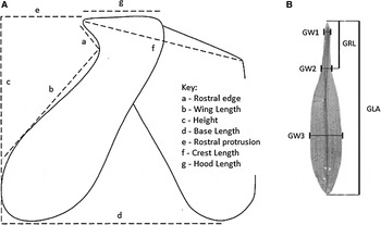
Fig. 3. Hard structure morphometric measurements recorded for Loligo reynaudii in this study, based mainly on the work by Clarke (Reference Clarke1986). (A) lower beak dimensions (taken from Ogden et al., Reference Ogden, Allcock, Watts and Thorpe1998), (B) Gladius dimensions (taken from Baron & Re, Reference Baron and Re2002).

Fig. 4. Diagram of a Loligo reynaudii statolith. (A) basic terms of a L. reynaudii statolith (after Jereb & Roper, Reference Jereb and Roper2010), (B) L. reynaudii statolith dimensions measured in this study (modified from the work by Clarke & Maddock, Reference Clarke, Maddock, Clarke and Trueman1988; Lipinski et al., Reference Lipinski, Roeleveld, Underhill, Okutani, O'Dor and Kubodera1993).
Table 1. Loligo reynaudii soft part and hard structure morphometric characters measured in this study.

All soft part morphometric data were measured to the nearest millimetre according to recommendations by Roper & Voss (Reference Roper and Voss1983), using a single set of vernier callipers. Measurements on the gladius and sucker rings were made after removing the structures from the squid. Gladius measurements were made to the nearest mm using vernier callipers and sucker ring diameter was measured using a low-powered microscope with an eyepiece micrometer. Beaks were carefully extracted from the buccal mass following the method described by Clarke (Reference Clarke1986) and immediately frozen until further analysis. After defrosting at room temperature at a later stage, lower beaks were measured in profile to the nearest 0.01 mm using a single set of digital callipers. Statoliths were removed from the head with a small pair of tweezers and stored in empty vials until further analysis of only one statolith per pair (either left or right) under a low-powered microscope with an eyepiece micrometer.
Analysis of morphological data
Prior to analysis, morphometric data were screened for errors using bivariate plots and regression analyses to identify outliers. Unfortunately soft part measurements could not be retaken as specimens were discarded after measurements. Errors in soft part data were therefore corrected by reference to the original data sheets, alternatively data from those samples were deleted. Some hard structures such as beaks and statoliths were re-measured where necessary.
Morphometric studies, whereby multivariate measurements of different body parts are used to characterize the average shape of the sampled population, need to take into account/adjust the effect of body size as most of the variations are the result of changes in body size (Lleonart et al., Reference Lleonart, Salat and Torres2000). There are slightly different ways of removing the effect of body size. In this study, each morphometric character was log-transformed and standardized using the following allometric formula (Liao et al., Reference Liao, Liu and Hung2010):
 $${M_{{\rm std}}} = \log (M) - \beta (\log (Ml) - (\log (\bar Ml))$$
where M
std is the standardized morphometric measurement, log(M) is the log of the morphometric measurement, β is the slope of regression of the morphometric measurement to the dorsal mantle length, Ml, log(Ml) is the log of the dorsal mantle length, and
 ${\rm log}(\bar Ml)$
is the mean of the log of the dorsal mantle length. Although this is the commonly used approach to remove the effect of size we have also considered another method that uses a size variable of each morphometric group, such as c for beaks and TSL for statoliths. The classification models were then applied to data of both approaches to remove the effect of size. Results of the classification, using the three models, were comparable (online Appendix B).
${\rm log}(\bar Ml)$
is the mean of the log of the dorsal mantle length. Although this is the commonly used approach to remove the effect of size we have also considered another method that uses a size variable of each morphometric group, such as c for beaks and TSL for statoliths. The classification models were then applied to data of both approaches to remove the effect of size. Results of the classification, using the three models, were comparable (online Appendix B).
SEXUAL DIMORPHISM
To test for sexual dimorphism Multivariate Analysis of Variance (MANOVA) was applied on the standardized measurements of soft body parts, beaks, statoliths and sucker rings. The assumption of normality and homogeneity of variance were checked visually using qqplot and plot of residuals vs fitted values respectively. In addition, we have also compared the slopes of the regression of different morphometric measurements vs dorsal mantle length for males and females in all three regions.
CLASSIFICATION OF SAMPLES
Prior to assessing the distinction between samples collected from the three different regions an exploratory analysis was conducted. This included a graphical summary of the morphometrics by sex and region, and a principal component analysis of the morphometrics. A number of statistical techniques are commonly used in the classification of samples. Based on sets of variables/attributes, these include: Discriminant Function Analysis (e.g. linear and quadratic), Classification Tree Analysis (CTA), Artificial Neural Network (ANN), Random Forest (RF), Support Vector Machine (SVM),…etc. In this study we have used Linear Discriminant Function Analysis (LDA), CTA and RF. Classification studies on Patagonian squid Doryteuthis gahi samples from different regions have shown samples to be less distinct when combining soft parts and hard structures (Vega et al., Reference Vega, Rocha, Guerra and Osorio2002). Thus all three statistical techniques were applied to the combination of all soft parts, and then to each of the different hard structures (lower beak, gladius, sucker rings and statolith) separately. In addition, data for males and females were analysed separately due to the apparent sexual dimorphism.
LINEAR DISCRIMINANT ANALYSIS (LDA)
In principle, Discriminant Analysis is similar to Principal Component Analysis (PCA) in that they both aim to find the optimal rotation when projecting observations. The main difference is in the way they extract major axes of variation. In PCA the objective is to extract a series of orthogonal axes that cumulatively extract most of the variation in the data, whereas in LDA we are interested in extracting sets of axes (usually two) that maximize the separation of a priori known groups (Zuur et al., Reference Zuur, Ieno and Smith2007). Unlike PCA there are a number of assumptions to be met for the results of LDA to be valid. These include variables to be on a continuous scale (categorical variable to be avoided as much as possible); the number of observations per group to be at least 2 but preferably 4 to 5 times the number of variables; the variables considered in the analysis to be linearly related but not with sets of variables with correlation coefficient of 1/−1; homogeneity of variance across groups (variance/variability of each of the variables considered to be roughly comparable across groups); as the method is based on the calculation of a covariance matrix that is pooled across groups, relationship among variables considered should be the same across groups; assumes independence of observations and multivariate normality (hence variables in each group are expected to be normally distributed). The most important assumptions are homogeneity of variance (required for the validity of the method itself due to the use of pooled covariance) and the normality of variables (required for hypothesis testing) (Zuur et al., Reference Zuur, Ieno and Smith2007).
CLASSIFICATION TREE ANALYSIS (CTA)
CTA is a non-parametric technique using recursive partitioning algorithm. The technique is widely used in fields ranging from social to medical sciences and has only relatively recently been recognized as a powerful method in ecology (De'ath & Fabricus, Reference De'ath and Fabricus2000), mainly because it naturally deals with non-linearity and higher-order interactions among predictors, which are the characteristics of most ecological data. The technique is also invariant to monotonic transformation of predictors, able to handle missing values in both response and predictor variable(s), making it is easy for interpretation (James et al., Reference James, Witten and Hastie2014). CTA explains the variation in the response variable by repeatedly partitioning the data into more homogenous groups using a combination of predictor variables. The algorithms repeatedly split data into a nested series of groups that are as homogenous as possible with respect to the response variable considered. In the context of classification problems (in this case classification of samples from three regions) the model starts with the whole data set, the root node, and formulates splitting rules for each value of the predictor variables to create candidate splits. The algorithm then selects the candidate splits that results in the smallest misclassification error rate using it to split data into two sub-groups. The algorithm then continues to recursively split the sub-groups until no split leads to substantial reduction in misclassification error rate or the number of observations in the sub-groups are too small for further splitting. When the algorithm cannot split a node further then it has reached the terminal/leaf node. CTA tends to over-fit which can usually be avoided by running tree-based sets of criteria in this using cross-validated error rates on the training data. Determination of the optimal size of tree was done via cross validation. The optimal size of the tree was selected based on the complexity parameter cp, and the complexity parameter that gave the lowest cross-validation error (and hence size of the tree) was selected. By applying the one Standard deviation rule the value of the cp (optimal tree size) was selected. Details of the method, implementation of the algorithm and examples are given in Zuur et al. (Reference Zuur, Ieno and Smith2007), Horton & Kleinman (Reference Horton and Kleinman2010) and James et al. (Reference James, Witten and Hastie2014).
RANDOM FOREST (RF)
Random forest is one of the developments in the area of predictive statistics together with bagging and boosting meant to improve classical tree models. Bagging (bootstrap aggregation) involves the construction of multiple trees based on the training set and finally aggregating the results to produce the final outcome. Although dissimilar, boosting involves creating many trees, not as an independent one but by repeatedly growing/updating the existing tree, and finally predicting the outcome. Random forest on the other hand improves both classical trees and bagging more so on classical trees. Similar to bagging, random forest creates multiple trees from the training data but does so by building the trees based on a random subset of the predictors that de-correlates the multiple tree created. This tends to make the trees less variable and more reliable (Hastie et al., Reference Hastie, Tibshirani and Friedman2009; James et al., Reference James, Witten and Hastie2014). Random forest is important in classification problems when there are large numbers of correlated predictors. Results from random forest is equivalent to that from bagging when the size of the number of variables selected for splitting equals the total numbers of predictors.
MODEL SELECTION AND PERFORMANCE
Mode selection was achieved using the step-wise selection approach. We specifically applied selection in both directions for all three model types. A combination of variables that lead to an increase in the overall classification rate with a cut-off threshold of 1% was selected to make the variable sets in the final model. The relative importance of predictors were assessed by the improvement in the overall classification rate achieved as a result of the addition of predictors.
Model predictive performance was assessed using re-sampling. There are different re-sampling techniques, specifically we have used the ‘Leave Group out Cross Validation’ LGOCV (also known as Monte Carlo cross validation) whereby each model is repeatedly trained on a subset of data to evaluate the remaining subset (Kuhn & Johnson, Reference Kuhn and Johnson2013). Predictive performance was then summarized as the mean ±1 SD of the predictive accuracy from the LGOCV.
Genetic analysis
Genomic DNA was extracted from tentacle tips using a CTAB-chloroform/IAA method (Winnepenninckx et al., Reference Winnepenninckx, Backeljau and Dewachter1993). Individuals were then genotyped at four microsatellite loci (Lfor1, Lfor3, Lrey44 and Lrey48) following Shaw et al. (Reference Shaw, Hendrickson, McKeown, Stonier, Naud and Sauer2010).
Genetic variability was assessed using numbers of alleles (N A ), observed heterozygosity (H O ) and expected heterozygosity (H E ) (Nei, Reference Nei1978), all calculated using FSTAT 2.9.3.2 (Goudet, Reference Goudet1995). Genotype frequency conformance to Hardy–Weinberg equilibrium (HWE) expectations and genotypic linkage equilibrium between pairs of loci were tested using exact tests incorporating a Markov chain method (Guo & Thompson, Reference Guo and Thompon1992) with default parameters in GENEPOP 3.3 (Raymond & Rousset, Reference Raymond and Rousset1995). Locus-by-sample combinations were tested for the presence of null alleles using MICROCHECKER (van Oosterhout et al., Reference van Oosterhout, Hutchinson, Derek and Shipley2004) with significant effects adjusted for using the van Oosterhout algorithm. Tests of genetic differentiation were then performed with and without null allele correction (NAC). Using FSTAT, genetic differentiation was quantified using the unbiased F ST estimator, θ (Weir & Cockerham, Reference Weir and Cockerham1984), calculated globally (over all samples) and between pairs of samples, with significance of estimates inferred following 10,000 permutations (Goudet et al., Reference Goudet, Raymond, de Meeus and Rousset1996) of genotypes among samples. Global and pairwise exact tests of allele frequency homogeneity were performed for each locus in GENEPOP with default Markov chain parameters. Multilocus values of significance were obtained by Fischer's method.
An important consideration when sampling highly mobile adults is the possible effect of sampling migrants on estimates of population structure derived from comparisons between admixed samples. To address this potential issue population structure was also investigated using the Bayesian clustering analysis implemented in the program STRUCTURE (Pritchard et al., Reference Pritchard, Stephen and Donnelly2000) which permits estimations of the most probable number of populations represented by the data without a priori sample definition. Both the ‘no admixture model’ (as recommended for low F ST; Pritchard et al., Reference Pritchard, Stephen and Donnelly2000) and ‘admixture model with correlated allele frequencies’ were used independently to identify the number of clusters, K (from a range of 1–5), with the highest posterior probability. Each MCMC run consisted of a burn-in of 106 steps followed by 5 × 10⁶ steps. Three replicates were conducted for each K to assess consistency. The K value best fitting the data set was estimated by the log probability of data [Pr(X/K)].
RESULTS
Morphology
REMOVAL OF THE EFFECT OF SIZE
Figure 5 shows the slope of the regression of soft body part variables vs DML that was used to remove the effect of size on the different morphometric measurements. The figure mainly highlights the difference between males and females suggesting sexual dimorphism. Similar patterns were observed for beaks, statoliths and sucker ring variables (not shown here due to space limitation but given in online Appendix C). Table 2 shows the results of the MANOVA applied to all morphometric measurements. It shows that in all cases the shape, as characterized jointly by all variables, of the soft body parts, beaks, statoliths and sucker rings differed among the three regions between sexes. In addition, for both soft body parts and beaks there was interaction between the region and sex suggesting the presence of not only sexual dimorphism but also variance among the three different regions.

Fig. 5. Plot of the slopes and the 95% confidence interval of the regression of Loligo reynaudii soft part measurements vs DML.
Table 2. Results of the MANOVA applied to all morphometric measurements taken for Loligo reynaudii in this study.

CLASSIFICATION OF SAMPLES
Result of the exploratory analysis applied to the morphometric measurements are shown in Figures 6A, B, 7–9. The figures show distinct differences between males and females and to some extent among the three regions, more so in the soft body part measurements. For the sake of comparison we present Figure 10. This figure shows the results of the PCA and LDA applied to the same morphometric data for the soft body part measurements. The LDA plots suggest distinction in the body shape of individuals sampled from the three regions. In contrast, the PCA ordination of the same data did not show such distinction among individuals collected from the different regions. This is largely a reflection of the way PCA extracts different PC axes: orthogonal axes that maximize the variance whereas LDA extracts axes that maximize the separation among groups that are a priori defined (in this case the regions where individual squids were sampled). Similar exploratory comparative multivariate analysis of beak, statolith and sucker ring data are shown in online Appendix D (not shown here due to space limitation).

Fig. 6. (A) Box–whisker plots of standardized values of attributes for the soft body parts of Loligo reynaudii males and females from the three regions. (B) Box–whisker plots of standardized values of attributes for the soft body parts of Loligo reynaudii males and females from the three regions, continued.

Fig. 7. Box–whisker plots of standardized values of attributes for the beaks of Loligo reynaudii males and females from the three regions.

Fig. 8. Box–whisker plots of standardized values of attributes for the statoliths of Loligo reynaudii males and females from the three regions.

Fig. 9. Box–whisker plots of standardized values of attributes for the sucker rings of Loligo reynaudii males and females from the three regions.

Fig. 10. Top: PCA ordination of Loligo reynaudii male (left) and female (right) individuals based on soft body part attributes. Bottom: LDA ordination of the same data for males (left) and females (right).
MODEL SELECTION AND PERFORMANCE
The best model was selected based on the step-wise approach. As shown in Table 3, for each of the four types of morphometric measurements (soft body parts, statoliths, beaks, and sucker rings) the three models appear to mostly select fewer numbers of variables given the sets of variables available (more so for the soft body parts). In addition, the type and number of variables selected by the different models appear to differ. For the soft body parts the FL was the most commonly selected variable by the three variables and for both sexes. The number and types of variables selected for the beak measurements differed among models. The same was observed for sucker ring measurements. For statolith measurements the type of variables selected differed among models but CTA and RF appear to select at least the same types of variables.
Table 3. Selection of Loligo reynaudii soft and hard part variables based on the stepwise-selection procedure.

Figures 11–14 show comparative performance of the three models for males and females separately and when combined. With the exception of the soft body part measurements (Figure 11), where the three models performed relatively well, both the overall accuracy of the models and their relative performance was different (Figures 12–14). The most accurate and higher classification of samples from the three regions were achieved using soft body parts (Figure 11). For males and females, and for both sexes combined, LDA and CTA performed very well followed by RF. The comparative performance of the three models based on variables from the beaks shown in Figure 12 highlights the low classification accuracy of the models and indicates lower predictive power of beak variables in the classification of samples from the three regions. A similar pattern was observed in the classification of samples based on statolith and sucker ring variables (Figures 13 and 14 respectively). Figure 15 shows how the soft body part phenotypic differences were more accentuated between samples from the Angola–Benguela Frontal zone (southern Angola) and the southern Benguela Current system (West Coast and Western Agulhas Bank), than between samples from the latter and the Agulhas Current system (central and eastern Agulhas Bank).

Fig. 11. Comparison of the predictive performance of the three models for Loligo reynaudii males, females, and combined individuals from the three regions based on attributes of soft body parts. The performance of the models on both the training and validation sets are shown.

Fig. 12. Comparison of the predictive performance of the three models for Loligo reynaudii males, females, and combined individuals from the three regions based on attributes of beaks. The performance of the models on both the training and validation sets are shown.

Fig. 13. Comparison of the predictive performance of the three models for Loligo reynaudii males, females and combined individuals from the three regions based on attributes of statolith. The performance of the models on both the training and validation sets are shown.

Fig. 14. Comparison of the predictive performance of the three models for Loligo reynaudii males, females and combined individuals from the three regions based on attributes of sucker ring. The performance of the models on both the training and validation sets are shown.

Fig. 15. The multivariate distance among samples of all Loligo reynaudii variables between each of the three regions.
Genetics
The total number of alleles per locus ranged from 18 to 28 (mean 23.5, SD 4.1) and levels of genetic variability were similar across samples (Table 4). All tests of linkage disequilibrium were non-significant indicating that the microsatellite loci are unlinked and thus provide independent estimates of population diversity. Lrey44 and Lrey48 exhibited significant deviations from HWE due to heterozygote deficits in all samples. A significant heterozygote deficit was also reported at locus Lfor1 in the Cape St. Francis (inshore) sample. All remaining locus/sample tests conformed to HWE expectations.
Table 4. Indices of genetic variation within Loligo reynaudii samples genotyped at four microsatellite loci.

N, sample size; HE, multilocus expected heterozygosities; HO, multilocus observed heterozygosities; NA, mean number of alleles per locus.
Global differentiation was significant when tested by exact test without NAC (P = 0.0027) but the corresponding test was not significant when performed with NAC (P = 0.1099). Global differentiation as measured by θ ST was not significant for both null allele corrected (θ ST = −0.004; P = 0.9990) and uncorrected data (θ ST = 0; P = 0.9110). Estimates of θ ST between pairs of samples were also low with no comparison significant when tested by permutation for either uncorrected or with NAC data (Table 5). Pairwise exact tests yielded a number of significant outcomes, with five out six significant results (for uncorrected data) involving the Plettenberg Bay (offshore) sample (Table 6). With NAC, only two pairwise comparisons were significant, both involving the Plettenberg Bay (offshore) sample. The Bayesian clustering method did not detect any significant population structure with unanimous support for models of K = 1 in all runs.
Table 5. Pairwise estimates of genetic differentiation (ΘST) between Loligo reynaudii samples, without (above diagonal) and with (below diagonal) null allele correction. No ΘST was significant when tested by permutation.

WC, West Coast; WAB, Western Agulhas Bank; MB, Mossel Bay; PB, Plettenberg Bay; SF, St Francis; PE, Port Elizabeth.
Table 6. P values from exact tests of genetic differentiation between Loligo reynaudii samples, without (above diagonal) and with (below diagonal) null allele correction. Significant values in bold, and values that remain significant after Bonferroni correction (underlined).

WC, West Coast; WAB, Western Agulhas Bank; MB, Mossel Bay; PB, Plettenberg Bay; SF, St Francis; PE, Port Elizabeth.
DISCUSSION
A number of methodological concerns encountered in the course of the study should be considered. For comparative morphometric studies, Pierce et al. (Reference Pierce, Thorpe, Hastie, Brierly, Guerra, Boyle, Jamieson and Avila1994a, Reference Pierce, Hastie, Guerra, Thorpe, Howard and Boyleb) recommended simultaneous sampling to minimize mixed-stock samples. In this case, samples for all three regions should ideally have been collected at least in the same season. However, due to the cost of sampling and large sampling area covered, it was not possible to collect all samples in the entire geographic range simultaneously or even during the same season. As squid are believed to be highly mobile (Boyle, Reference Boyle1990), this may have had a temporal effect on the results of the morphometric analyses and should be kept in mind when interpreting results.
A difference in morphological characteristics between L. reynaudii sampled in South Africa and Angola is perhaps not surprising, with the exception of soft body part phenotypic differences being more accentuated between samples from the Angola–Benguela Frontal zone and the southern Benguela Current system, than between samples from the latter and the Agulhas Current system. Given the break in distribution of L. reynaudii in Namibian waters, a much higher degree of mixing between individuals from the Agulhas Current and the southern Benguela Current than between the latter and southern Angola would be assumed. However, given the highly mobile nature of both larvae and adults, one would intuitively expect a single stock along the South African coast. Populations occurring on the West Coast and western Agulhas Bank vs those occurring on the central and eastern Agulhas Bank however may also be phenotypically distinct from each other due to the different environmental conditions found on either side of Cape Agulhas. The corresponding genetic data support high gene flow throughout this region and suggest that the subtle differentiation reported by Shaw et al. (Reference Shaw, Hendrickson, McKeown, Stonier, Naud and Sauer2010) does not reflect temporally stable population sub-structuring but rather temporary random variation within a single population. This implicates environmental heterogeneity and not population isolation as a driver of the phenotypic divergence.
Temperature regimes can have a significant influence on the growth and development of cuttlefish and squid, and growth at different temperatures can result in squid of markedly different size and growth-related parameters (Forsythe et al., Reference Forsythe, Derusha and Hanlon1994, Reference Forsythe, Walsh, Turk and Lee2001; Carvalho & Nigmatullin, Reference Carvalho, Nigmatullin, Rodhouse, Dawe and O'Dor1998). According to Pörtner & Zielinski (Reference Pörtner and Zielinski1998), oxygen availability can also limit performance levels in squid. Some squid may be able to operate at their functional and environmental limits, revealing a trade-off between oxygen availability, temperature, performance level, growth and possibly body size (Pörtner & Zielinski, Reference Pörtner and Zielinski1998). Conditions on the west coast (southern Namibia, west coast of South Africa and the western Agulhas Bank, 29°–35°S) are influenced by the cold equator-ward flowing Benguela current and associated with much colder bottom water temperatures fluctuating between 5° and 11°C with an average of 10°C, and low bottom dissolved oxygen (BDO) of 1.5–4.5 ml 1−1 (Augustyn, Reference Augustyn1991; Roberts, Reference Roberts2005). It is likely that the Lüderitz upwelling cell off the coast of southern Namibia acts as a partial environmental barrier to movement of squid. On the south coast (central and eastern Agulhas Bank, 20°–26°E) of South Africa, conditions are influenced by the warm south-westward flowing Agulhas current and associated with moderate water temperatures fluctuating between 9° and 24°C, and well oxygenated bottom waters (Augustyn et al., Reference Augustyn, Lipinski, Sauer, Roberts and Mitchell-Innes1994). Therefore, given that water temperature and bottom dissolved oxygen considerably differ in each region, they may act as the main drivers of phenotypic variation found in chokka L. reynaudii from the different regions. However, better defined and substantiated relations need to be further researched.
In contrast to the findings of Borges (Reference Borges1995), Vega et al. (Reference Vega, Rocha, Guerra and Osorio2002) and Martinez et al. (Reference Martinez, Sanjuan and Guerra2002), soft parts in this study proved to be more effective than hard structures (gladius, lower beaks, sucker rings, statoliths) in discriminating between squid populations from different geographic regions. This is surprising as soft body parts are generally accepted as being less reliable than hard structures due to their plasticity and warping response to freezing and thawing (Carvalho & Nigmatullin, Reference Carvalho, Nigmatullin, Rodhouse, Dawe and O'Dor1998). Nevertheless, as pointed out earlier, the geographic variation found in L. reynaudii soft body parts may be related to phenotypic responses derived from region-bound environmental conditions (Shea & Vecchione, Reference Shea and Vecchione2002). This is an evolutionary phenomenon that has been identified in other species of squid occurring in different habitats across large geographic areas (Carvalho & Pitcher, Reference Carvalho and Pitcher1989; Hernandez-Garcia & Castro, Reference Hernandez-Garcia and Castro1998; Vega et al., Reference Vega, Rocha, Guerra and Osorio2002).
In conclusion the study demonstrated some phenotypic population sub-structuring of Loligo reynaudii. LDA demonstrated that morphologically there is some evidence that squid from the south coast (central and eastern Agulhas Bank), west coast (west coast and western Agulhas Bank) and southern Angola are different. The diverse marine environment was postulated to be one reason for this variation. Molecular analysis did not support the existence of a genetic breakpoint allowing a geographic reference point for separating stocks. While the potential disconnect between genetic and demographic connectivity (i.e. low migration rates may be sufficient to homogenize genetic variation but be insufficient to prevent independent reaction of populations/stocks) is an important consideration for management, data indicate that the regional patterns of morphological divergence are occurring against a background of high gene flow. This pattern confirms the influence of environmental heterogeneity and not restriction of genetic flow/isolation as the primary driver of the phenotypic divergence. The observed phenotypic heterogeneity probably reflects the interplay between genetic adaptation and short-term plasticity, which may vary through the studied range. Although cephalopods are renowned for their phenotypic plasticity, the phenotypic divergence may reflect adaptive differences which may be important for future sustainability and management of this resource. Further targeted experimental investigations will be needed to determine the exact underlying drivers of the phenotypic divergence. Furthermore, recent advances in molecular techniques may also help to link phenotypic and genomic variation and improve understanding of the roles of adaptation and plasticity (Allendorf et al., Reference Allendorf, England, Luikart, Ritchie and Ryman2008). Discovered phenotypic differences may signal the beginning of the evolutionary divergence between various geographic groupings (eventually resulting in differences between hard parts, and genetic splits), but they are insufficient at this stage to revise the current management strategy of the chokka squid resource.
SUPPLEMENTARY MATERIAL
To view supplementary material for this article, please visit http://dx.doi.org/10.1017/s0025315415001794
ACKNOWLEDGEMENTS
All our colleagues at the Department of Agriculture, Forestry and Fisheries (DAFF), and the South African Squid Management Industrial Association (SASMIA) who provided for and assisted with the collection of squid samples during research cruises.
FINANCIAL SUPPORT
This work was supported by the South African Squid Management Industrial Association and Rhodes University.


