INTRODUCTION
The abrupt topography of seamounts in all oceans provides particular habitats of hard substrata and soft bottom for the benthic fauna as well as for associated pelagic communities, in contrast to the general flat and sediment-covered deep-sea plains (Rogers, Reference Rogers1994; Stocks & Hart, Reference Stocks, Hart, Pitcher, Morato, Hart, Clark, Haggan and Santos2007). In the water column, current–topography interactions between seamounts and the surrounding oceanic flows may generate meso-scale variability and affect the local retention time of water masses, including particles, phytoplankton and smaller zooplankton (Genin & Boehlert, Reference Genin and Boehlert1985; Roden, Reference Roden1994; Lavelle & Mohn, Reference Lavelle and Mohn2010). The uplift of deeper nutrient-rich water associated with the biological retention potential of seamounts may be increased by hydrodynamic processes such as seamount associated eddies (Richardson, Reference Richardson1980, Reference Richardson1981), Taylor caps/columns or tidal resonance and seamount-trapped waves (see White et al., Reference White, Bashmachnikov, Arístegui, Martins, Pitcher, Morato, Hart, Clark, Haggan and Santos2007; Lavelle & Mohn, Reference Lavelle and Mohn2010).
Despite the hypothesis of seamounts as places of enhanced biomass and production (Rogers, Reference Rogers1994), only limited evidence suggests that seamounts can support elevated biomass and abundance of the benthic invertebrate fauna (see Genin, Reference Genin2004; Clark et al., Reference Clark, Rowden, Schlacher, Williams, Consalvey, Stocks, Rogers, O'Hara, White, Shank and Hall-Spencer2010; Rowden et al., Reference Rowden, Schlacher, Williams, Clark, Stewart, Althaus, Bowden, Consalvey, Robinson and Dowdney2010). However, it has been demonstrated by Mullineaux & Mills (Reference Mullineaux and Mills1997) that current–topography interactions can retain larvae in seamount-associated flows, which is likely to affect the recruitment of the benthic population. Boehlert & Mundy (Reference Boehlert and Mundy1993) assumed seamounts as sources of eggs and larvae leading to assemblages of ichthyoplankton. Though meroplanktonic larvae, belonging to the micro- and mesozooplankton community, are an important factor for recruitment, food supply and production in a seamount ecosystem, related studies are sparse (e.g. Mullineaux & Mills, Reference Mullineaux and Mills1997; Metaxas, Reference Metaxas2011).
The microzooplankton community, usually defined as the size fraction 0.02–0.2 mm, includes protists such as ciliates and foraminiferans, but also metazoan larvae and small metazoans like small copepods and nauplius and copepodite stages of copepods. We also consider dinoflagellates as part of the microzooplankton here (Sherr & Sherr, Reference Sherr and Sherr2007). In particular the small developmental stages of copepods are an important prey for fish larvae and other zooplanktivorous consumers (Turner, Reference Turner2004), and on the other hand exert an important grazing impact on phytoplankton communities, which are seasonally dominated in low latitudes by extremely small cells of nano- and picoplankton (Landry et al., Reference Landry, Constantinou and Kirshtein1995). However, there is still little knowledge on the small zooplankton groups and their trophic position in the marine food web as compared with, for example, larger copepod taxa, because the small-sized zooplankton has usually been undersampled in the oceanic realm due to the common usage of nets with mesh sizes >0.2 mm (Gallienne & Robins, Reference Gallienne and Robins2001; Turner, Reference Turner2004).
Using a multiple opening and closing net system with a mesh size of 0.055 mm, the present study assesses the spatial distribution of microzooplankton in relation to the mesozooplankton fraction at Ampère and Senghor, two shallow seamounts in the subtropical and tropical NE Atlantic, with special attention to the abundance of invertebrate larvae. In particular we were interested whether and where microzooplankton is accumulated over Ampère and Senghor. The study further addresses the question whether meroplanktonic larvae are retained in seamount surrounding waters as proposed by Mullineaux & Mills (Reference Mullineaux and Mills1997) and whether the seamounts may be considered as hotspots in the open ocean for larvae from benthic invertebrates, such as corals, gastropods, bivalves, polychaetes and echinoderms, which have been sampled during cruises to Senghor in September/October 2009 and to Ampère in May 2005 and in November/December 2010 (Beck et al., Reference Beck, Metzger and Freiwald2006; Christiansen & Koppelmann, unpublished data; Molodtsova & Vargas, unpublished data; Chivers et al., Reference Chivers, Narayanaswamy, Lamont, Dale and Turnewitsch2013). Complementary to our previous study on mesozooplankton (Denda & Christiansen, Reference Denda and Christiansen2014), we focus on small-sized zooplankton and give an assessment of the respiratory carbon demand and the taxonomic composition in order to better understand the trophic position of the microzooplankton and their impact on the phytoplankton community in the oligotrophic system of the NE Atlantic subtropical gyre as compared with the mesotrophic system of the tropical gyre. In this context we addressed the following questions:
-
(a) How do the local current regime and the hydrographic conditions affect the microzooplankton distribution in distinct seamount regions (summit plateau, rim, slope, up- and downstream sides) compared with open ocean reference sites in terms of biomass and abundance?
-
(b) How does the large-scale current regime of the subtropical and tropical gyre affect the microzooplankton distribution at Ampère and Senghor Seamounts, respectively, in terms of biomass, abundance and respiratory carbon demand?
-
(c) Are Ampère and Senghor Seamounts hotspots for benthic invertebrate larvae, featuring enhanced larval abundance as compared with the open ocean?
MATERIALS AND METHODS
Study sites
AMPÈRE SEAMOUNT
Ampère Seamount was sampled during cruise M83/2 of RV ‘Meteor’ in November/December 2010. Ampère, within the sphere of the NE Atlantic subtropical gyre, belongs to the Horseshoe Seamounts Chain, which is located between the island of Madeira and the Portuguese mainland ~360 NM west of the Strait of Gibraltar at 35°02′N 012°54′W (Figure 1). The current regime around Ampère is mainly driven by the Azores current and the Mediterranean outflow. The seamount rises from a base depth at 4500 m to a summit depth at 120 m with one small peak rising to 55 m (Figure 2A), partially overgrown with macroalgae in the photic zone (Christiansen, unpublished data). The seamount has a conical shape with a small, rough summit plateau and steep rocky slopes and canyons (Kuhn et al., Reference Kuhn, Halbach and Maggiulli1996; Hatzky, Reference Hatzky and Wille2005) as well as sediment-covered areas. For comparison, one open ocean reference station (hereafter referred to as ‘far field’) ~70 NM south-west of Ampère Seamount, located at 33°48′N 013°00′W, was also sampled. Water depth was about 4400 m over a flat sedimentary plain.

Fig. 1. Locations of Ampère and Senghor Seamounts and the far field sites (FF) in the NE Atlantic. Bathymetric data source: GEBCO (IOC et al., 2003).

Fig. 2. (A) Bathymetry and sampling locations of CTD and MultiNet® at Ampère Seamount on cruise M83/2 in November/December 2010 (credit bathymetric data: J. Hatzky, AWI). (B) Bathymetry and sampling locations of CTD and MultiNet® at Senghor Seamount on cruise P423 in December 2011 and P446 in February 2013 (credit bathymetric data: A. Schmidt, IFM-GEOMAR).
SENGHOR SEAMOUNT
Senghor Seamount was sampled during the cruises P423 and P446 of RV ‘Poseidon’ in December 2011 and February 2013. Senghor is located ~60 NM east of the island of Sal, Cape Verde at 17°12′N 021°57′W (Figure 1). The ocean dynamics around Senghor are mainly characterized by the north equatorial current system which drives the NE Atlantic tropical gyre (see Mittelstaedt, Reference Mittelstaedt1991; Lathuilière et al., Reference Lathuilière, Echevin and Lévy2008) and by the Cape Verde frontal zone between North and South Atlantic central water (Zenk et al., Reference Zenk, Klein and Schröder1991). Water depth at the base of the seamount is about 3300 m; the minimum summit depth is 90 m (Figure 2B). Senghor Seamount has a nearly circular shape with a small summit plateau and features a heterogeneous surface structure, which was shown by several ROV dives during cruise M79/3 of RV ‘Meteor’ in September/October 2009 (Christiansen & Koppelmann, unpublished data). The summit plateau is covered with sediment in most parts but also shows rocky areas in the centre, and ripple marks indicate strong currents at a water depth of 100 m. At the edge of the summit plateau at a depth of 320 m the seafloor is also sediment-covered, but without ripple marks. Along the slopes down to the deep sea floor soft bottom alternates with rocky areas. For comparison, an unaffected open ocean reference station (hereafter referred to as ‘far field’) ~60 NM north of Senghor Seamount, located at 18°05′N 022°00′W, was sampled. Water depth was about 3300 m over the flat sedimentary plain.
Hydrographic data collection
CTD (Conductivity-Temperature-Depth) casts were performed around Ampère and Senghor seamounts and at the far field sites, using a Seabird CTD equipped with sensors for temperature, conductivity, oxygen and fluorescence. In our study we examined CTD stations in the proximity of the zooplankton sampling stations, covering the upper 100 m of the water column over the summit plateau and rim and the upper 1000 m of the water column over the mid slopes and at the far field sites (Figure 2A, B; Table 1).
Table 1. Haul data for CTD and MultiNet during expeditions to Ampère Seamount in November/December 2010 and to Senghor Seamount in December 2011 and February 2013.

Direct current velocity data were obtained from two vessel-mounted ADCP (Acoustic Doppler Current Profiler) surveys at Ampère (M83/2) and Senghor seamounts (P446). ADCP data were not collected during the P423 Senghor cruise due to technical problems. ADCP measurements were conducted with 38 kHz (M83/2) and 75 kHz (P446) Teledyne RDI Ocean Surveyor systems. Single ping velocity profiles were recorded along with corresponding records of position, heading and time. Depth bin size settings varied between 16 m (depth range 27–651 m, Ampère Seamount) and 8 m (depth range 22–814 m, Senghor Seamount). Two-minute ensemble velocity averages were created from all single ping ADCP velocity profiles. Further processing was carried out using the Common Oceanographic Data Access System (CODAS) developed by the University of Hawaii (Firing et al., Reference Firing, Ranada and Caldwell1995; http://currents.soest.hawaii.edu/docs/adcp_doc/index.html) and following the guidelines for shipboard ADCP measurements by the GO-SHIP group (Firing & Hummon, Reference Firing and Hummon2010). Individual processing steps included evaluation and correction (if applicable) of transducer misalignment, as well as estimating transducer orientation, velocity amplitude scale factor and navigation. Resulting ship speed estimates were used to calculate absolute currents. Depth bins with per cent good values less than 80% of the return signal were discarded. Owing to the heterogeneous data distribution, ADCP velocities at each depth bin were spatially interpolated over a uniform grid using the DIVA software (Data Interpolating Variational Analysis; Troupin et al., Reference Troupin, Machín, Ouberdous, Sirjacobs, Barth and Beckers2010). The grid size was set to 0.02° (~1 NM) in latitude and longitude. DIVA employs optimal interpolation and error analysis of spatially scattered data based on meaningful estimates for the spatial correlation length scale L and the signal to noise ratio λ. A characteristic seamount length scale (L = 0.2° inside the 1000 m isobath) was considered adequate to resolve the principal dynamic scales at both seamounts. λ was set to a constant and uniform value of order unity (λ = 1) to reduce potential artefacts in the interpolated velocity fields from the mismatch between high-resolution along-track and low-resolution cross-track measurements. The horizontal distributions of flows were plotted at particular depths roughly corresponding to the surface depth (43 and 38 m), the depth of the summit plateau (91 and 86 m), the lower rim of the plateau (251 and 246 m) and the mid slope (395 and 398 m) of Ampère and Senghor seamounts, respectively.
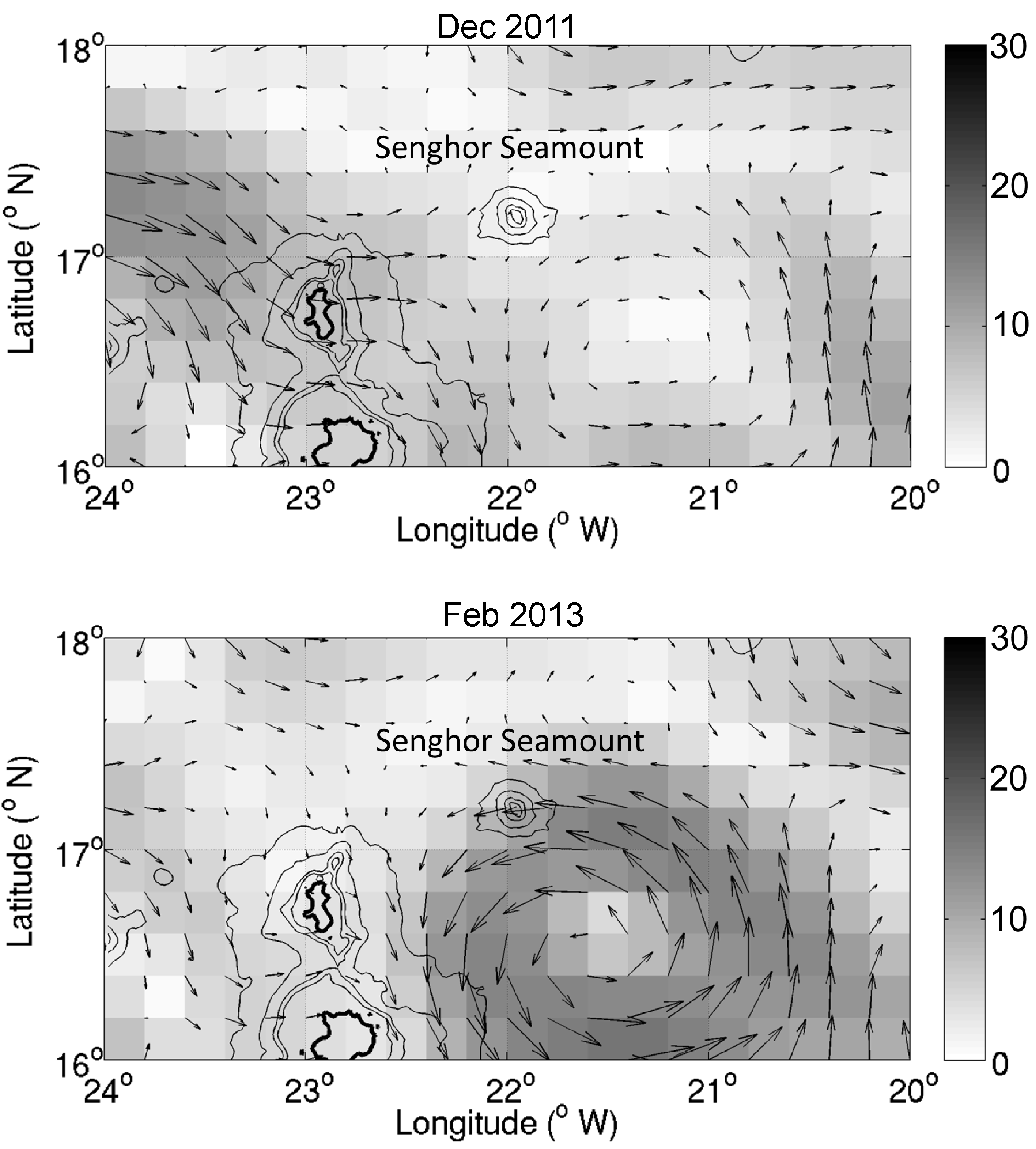
Monthly composites (December 2011, February 2013) of absolute geostrophic currents (cm s−1) were calculated from daily AVISO satellite altimetry (http://www.aviso.altimetry.fr/en/home.html) to compare major surface circulation features surrounding Senghor Seamount. The altimetry data analysed here are multi-mission datasets from up to four satellites at a given time on a 0.25° regular grid. The altimetry data processing and gridding methodology are described in detail in the SSALTO/DUACS User Handbook (2006).
Zooplankton sampling
Zooplankton were collected using vertical hauls with a Hydro-Bios 0.25 m2-MultiNet® (Weikert & John, Reference Weikert and John1981) equipped with five nets. The mesh aperture was 0.055 mm. The sampling design comprised a vertical profile at the far field station and two orthogonal transects across the seamounts, one in north-south and one in east-west direction, with stations at the mid slopes down to 1000 m depth, at the rim of the plateau and at the summit centre (Figure 2A, B; Table 1). The water column was subdivided into the following sampling intervals, depending on the maximum water depth: 1000–750–500–400–300–200–100–50–25–0 m. The net was lowered and hauled up with 0.5 m s−1. In order to achieve this vertical resolution with a five nets MultiNet® sampler at the slope stations, the 1000 m profiles were split into two casts, one from 1000 to 300 m and a second one from 300 m to the surface. During the Senghor surveys each cast was usually performed twice, in order to get two complete vertical profiles at each station, to allow for statistical analyses (Table 1). In 2011 one day and one night profile were obtained at each station, in 2013 samples were taken only during daytime. Due to technical problems of the ship, the sampling design could not be completed as planned, and some stations are missing from each cruise. At Ampère Seamount casts were performed only once independent of daytime due to lack of ship time.
Upon recovery of the MultiNet®, the nets were rinsed with seawater and the catch transferred into PE bottles. The material was preserved in a 4% formaldehyde-seawater solution buffered with borax for biomass determination and taxonomic identifications.
Biomass analyses and carbon demand
In the laboratory, the zooplankton samples were fractionated by sieving into the size classes 0.055–0.3 and 0.3–20 mm (hereafter referred to as ‘microzooplankton’ and ‘mesozooplankton’). The separation between micro- and mesozooplankton is usually 0.2 mm, but fractionating through a 0.3 mm sieve allowed an estimation of the importance of microzooplankton in comparison with previous data of the present study sites (Denda & Christiansen, Reference Denda and Christiansen2014) and with the often used 0.3 mm net samples focusing on calanoid copepods (e.g. Roe, Reference Roe1988; Wiebe et al., Reference Wiebe, Copley and Boyd1992; Fabian et al., Reference Fabian, Koppelmann and Weikert2005; Koppelmann & Weikert, Reference Koppelmann and Weikert2007). The wet weight of each size fraction was measured after removal of the interstitial water with 70% alcohol according to the method of Tranter (Reference Tranter1962). After wet weight determination the size fractions were split into two subsamples by a modified Folsom plankton splitter (McEwen et al., Reference McEwen, Johnson and Folsom1954). One half was transferred into sorting fluid (0.5% propylene phenoxetol, 5% propylene glycol and 94.5% H2O; Steedmann, Reference Steedmann and Steedmann1976) for counts and taxonomic analyses. For dry weight determination the other half was filtrated in a volume of 250 ml distilled water on a pre-combusted (at 500°C for 0.5 h) and pre-weighed fibreglass filter (Whatman GF/C, ø 45 mm), and oven-dried at 60°C for 24 h until the sample reached a stable weight.
The volume of the filtered water for each net was calculated by multiplying the net opening (0.25 m2) with the sampling interval as measured by the pressure sensor, assuming a filtration efficiency of 100%. Biomass (dry weight) was standardized to milligrams per 1 m3 (mg m−3). Standing stocks in terms of biomass integrated over the whole water column or a given depth range were calculated as mg m−2.
For the calculation of the respiratory carbon demand mean individual dry weight (mg Ind−1) was determined by dividing the dry weight of the sample by the number of individuals in the parallel sample. Individual respiration rates were calculated from mean individual dry weight and temperature for each sample, respectively, using a multiple-regression model after Ikeda (Ikeda et al., Reference Ikeda, Kanno, Ozaki and Shinada2001):
 $$\; {\rm ln}\;R = - 0.399 + 0.801\;{\rm ln}\;W + 0.069T$$
with R = individual O2 respiration rate (μl Ind−1 h−1); W = mean individual dry weight (mg Ind−1); T = mean temperature in sampling intervals (°C). The individual oxygen respiration rates (μl Ind−1 h−1) were multiplied by the total number of individuals (Ind m−3); the resulting community oxygen respiration rates (μl m−3 h−1) were then converted to carbon equivalents RC (μg m−3 h−1) by the equation:
 $$\; {\rm RC} = R*{\rm RQ}*12/22.4$$
where RQ is a respiratory quotient of 0.97 (Omori & Ikeda, Reference Omori and Ikeda1984; Ikeda et al., Reference Ikeda, Torres, Hernandez-Leon, Geiger, Harris, Wiebe, Lenz, Skjoldal and Huntley2000) and 12/22.4 is the weight (12 g) of carbon in 1 mole (22.4 L) of carbon dioxide (Ikeda et al., Reference Ikeda, Torres, Hernandez-Leon, Geiger, Harris, Wiebe, Lenz, Skjoldal and Huntley2000). Respiratory carbon demands for distinct depth layers were calculated as mg m−2 d−1. Since Ikeda's regression model refers only to epipelagic zooplankton, calculated respiration rates of zooplankton for the mesopelagic zone (300–1000 m) were reduced by 50% to consider the effect of pressure, following Ikeda et al. (Reference Ikeda, Sano, Yamaguchi and Matsuishi2006), who concluded that mesopelagic respiration rates were in the order of one-half that of epipelagic respiration.
Taxonomic analyses
Microzooplankton samples of M83/2 were split by a plankton splitter after Wiborg (Reference Wiborg1951), using a subsample of 1/5, 1/10, 1/20 or 1/25. Microzooplankton samples of P423 and P446 were split using a Stempel pipette. Depending on the total number of individuals, an aliquot of 2.5, 5 or 10 mL was removed by the pipette from the sample diluted in a conical flask of 250 mL. Mesozooplankton samples were split using a modified Folsom plankton splitter (McEwen et al., Reference McEwen, Johnson and Folsom1954) to a subsample of 1/2, 1/4, 1/8 or 1/16.
Protistan and metazoan zooplankton were sorted and counted under a dissecting microscope, identified at phylum, class or order level or at developmental stage and grouped as follows: Dinoflagellata, other Protista (Foraminifera and Tintinnina), Appendicularia, other pelagic non-Crustacea (Cnidaria, Mollusca, Polychaeta, Chaetognatha, Thaliacea), invertebrate larvae (without nauplii of holoplanktonic organisms, but including Cirripedia larvae), nauplii (including mainly Copepoda, but also Euphausiacea, Decapoda, which were not counted separately), and other pelagic Crustacea (Ostracoda, Cladocera, Hyperiidea, other Amphipoda, Decapoda, Euphausiacea, Mysidacea, other Harpacticoida). Copepoda were identified at the family, genus or species level, such as the most abundant Micro-/Macrosetella spp., Oithona spp., Oncaea spp., Paracalanidae and Clausocalanidae. Other less abundant or juvenile copepod taxa were grouped and presented in the graphic results as other Cyclopoida and other Calanoida, respectively. A particular focus was on the identification of invertebrate larvae of Cnidaria, Gastropoda, Polychaeta, Cirripedia and Echinodermata. Exoskeletons, according to Wheeler (Reference Wheeler1967) and Weikert (Reference Weikert1977), and fragments of gelatinous organisms like Siphonophora were not considered in this study.
Counts were multiplied by the division factor of the subsample, and abundance was standardized to individuals per 1 m3 (Ind m−3). Standing stocks integrated over the whole water column or a given depth range were calculated as Ind m−2.
Data analyses
Prior to the statistical analyses, data were log transformed [Y′ = log (Y + 1)] in order to reach approximate normal distribution and homogeneity of variances, tested using the Kolmogorov–Smirnov and the Levene tests, respectively. Biomass standing stocks of microzooplankton (mg m−2) and abundance standing stocks of meroplanktonic larvae (Ind m−2) were calculated for two depth layers: 0–100 and 100–1000 m, roughly corresponding to the epipelagic zone above the summit depths and the mesopelagic zone including the lower epipelagic. Within each layer differences in standing stocks of biomass and abundance between distinct seamount regions and the far field were tested statistically for locations with two replicate hauls available. One-way analyses of variance (ANOVA) (Lozán & Kausch, Reference Lozán and Kausch2004; Sokal & Rohlf, Reference Sokal and Rohlf2009) were used, followed by a priori hypothesis tests using contrasts to test for differences between distinct pairs of samples (summit vs. rim, summit vs. slope, rim vs. slope, up- vs. downstream, seamount vs. far field, Senghor2011 vs. Senghor2013, Ampère vs. Senghor2011, Ampère vs. Senghor2013).
All statistical tests were performed using the SYSTAT 8.0 statistical package (SPSS Inc., 1999). For clarity, only significant results of t-tests and ANOVAs/a priori tests are given in the text in form of t and F values, respectively, together with degrees of freedom and significance levels of P < 0.05 and P < 0.01. Full statistical results are available in the electronic supplement (Table S1–3).
In order to investigate similarities between distinct seamount regions and the far field in terms of zooplankton abundance standing stocks, multivariate analyses were performed by group-average linked cluster analysis and non-metric multi-dimensional scaling (MDS) using PRIMER 6 v. 6.1.6 (Clarke & Gorley, Reference Clarke and Gorley2006). All identified taxa and developmental stages were included, resulting in 24 groups for Ampère, 44 groups for Senghor in 2011 and 50 groups for Senghor in 2013. Abundance of each group was integrated over 0–100 and 100–1000 m depth, calculated as Ind m−2. Abundance standing stocks of the respective depth layer were square-root transformed and Bray–Curtis similarity matrices were calculated to generate clusters, which were described by non-metric MDS plots with 10 restarts to determine lowest stress giving a good ordination of similarities into the corresponding distance matrix. Statistically significant differences (P < 0.05) among groups of locations in the cluster analyses were determined by similarity profile tests (SIMPROF) (Clarke & Warwick, Reference Clarke and Warwick2001; Clarke & Gorley, Reference Clarke and Gorley2006).
Linkage between the physical and biological data was determined by the BEST (Biota and/or Environment matching) procedure using the BIO-ENV method (PRIMER 6 v. 6.1.6; Clarke & Gorley, Reference Clarke and Gorley2006). For each cruise physical and biological data of the slope stations, the summit and the far field were used. For Senghor2013 the rim stations were also included, but not for the other cruises since zooplankton or hydrographic data are missing. Physical variables included depth, temperature, salinity, oxygen and fluorescence from the CTD casts. For Ampère and Senghor2013, absolute current velocity and direction from the ADCP collections were also included. Mean values were calculated for each MultiNet® sampling interval. Physical variables except depth were log transformed [Y′ = log (Y + 1)] according to Clarke & Warwick (Reference Clarke and Warwick2001). The values for each physical variable were normalized, having their mean subtracted and being divided by their standard deviation, making it possible to derive meaningful distances between values of physical variables on completely different scales with arbitrary origins. Dissimilarity matrices of the physical variables were calculated by Euclidean distance. Biological data were square-root transformed and Bray–Curtis similarity matrices were calculated. The analyses were done on the abundances of all identified groups (Ind m−3) and, separately, on the abundance of meroplanktonic larvae (Ind m−3) as well as on micro- and mesozooplankton biomass (mg m−3) (mean values of parallel hauls). The BIO-ENV procedure then measures the matching entries of the physical and biological matrices by a Spearman rank correlation and selects the combination of physical variables which maximizes the correlation coefficient (Clarke et al., Reference Clarke, Sommerfield and Gorley2008).
RESULTS
Hydrography
Hydrographic conditions at Ampère Seamount and the far field site indicate a strong stratification of the water column during November/December 2010 (Figure 3). A homogeneous warm mixed surface layer extended over the upper 60–80 m with temperature ~18.6°C and salinity ~36.4 above the seamount. In the far field, temperature and salinity of the mixed layer were higher with 20.4°C and 36.7, respectively. An oxygen maximum occurred between 80 and 100 m in the far field with values of 7.5 ml L−1. Over the seamount slopes, oxygen concentrations reached 6.7–7.0 mL L−1 but without showing a distinct maximum. Over the shallow summit no oxygen increase was obvious. Coincident with the oxygen maximum, the relative fluorescence data in the far field showed a maximum at around 80 m. Due to technical failure fluorescence data are not available for the seamount. Below the mixed layer a steep gradient in temperature, salinity and oxygen extended over 20 m, followed by a gradual decrease of temperature and oxygen to 1000 m depth at all deep stations. In contrast, salinity increased below 600 m depth reaching maximum values of ≥36 at 1000 m depth. This deep salinity increase was more pronounced over the slopes than in the far field.

Fig. 3. Vertical profiles of temperature (T; °C), salinity (S), oxygen (O2; mL L−1) and fluorescence (F; Ampère: mg m−3; Senghor: RFU = relative fluorescence unit) for the summit, E and W slope and the far field of Ampère Seamount in November/December 2010 and Senghor Seamount in December 2011 and February 2013.
Over Senghor Seamount and at the corresponding far field site hydrographic conditions indicate a well stratified water column during both sampling seasons (Figure 3). Surface water temperature was ~24.5°C in December 2011 and ~22.1°C in February 2013, building a warm mixed surface layer in the upper 50–75 m with salinity values of 36.4 and 35.8, respectively. This layer was characterized by a distinct oxygen maximum of 4.6 mL L−1 and was markedly thinner above the summit and the eastern slope as compared with the western slope and the far field site in 2013. At the bottom of the mixed layer of the deep stations the relative fluorescence data (not available for far field 2011) show a deep maximum between 35 and 70 m, and salinity reached a peak of 36.8. A steep gradient in all parameters extended down to 150 m, marking the thermocline. Below 150 m, temperature decreased gradually to 6.3°C at 1000 m, and salinity to 34.9. Oxygen had a minimum of 1.3 mL L−1 at 400–500 m and increased gradually below this depth, reaching concentrations of >2 mL L−1 at 1000 m.
DIVA objective analysis was used to create gridded composites of all ADCP velocity profiles without removing the tidal component and each sampling period. The resulting maps represent realistic spatial and temporal snapshots of predominant flow characteristics during each sampling period provided that changes in flow patterns are sufficiently small. Below 400 m the general flow fields marginally changed at both seamounts. Analysis of geostrophic currents from daily AVISO altimetry indicated largely synoptic surface flow conditions at both seamounts at the time of sampling (for Senghor seamount see Figure S1 in the electronic supplement; Ampère Seamount not shown). However, the gridded ADCP data most likely underestimate the presence of higher frequency motions in the original data. Water current estimates from ADCP measurements at Ampère Seamount indicate generally south-eastward flow in the upper 100 m with maximum currents of 35 cm s−1 to the south of the seamount and 15–25 cm s−1 directly impinging at the seamount. Weaker currents (5–10 cm s−1) were observed downstream of the seamount at the eastern and south-eastern slopes (Figure 4A). At 251 m and 395 m depth the flow was ~10–15 cm s−1 to the east. At the northern slope of the seamount a deflection to the north/north-east was apparent at all depths, reaching magnitudes of 30–40 cm s−1 in the upper 100 m and 20 cm s−1 in deeper waters.

Fig. 4A. Gridded current velocities (cm s−1) at Ampère Seamount in December 2010 derived from 2 min ensemble averaged 38 kHz ADCP data from the M83/2 cruise using DIVA objective analysis. Flow vectors and current speeds are presented at four discrete depth levels (43, 91, 251, 395 m) and every third flow vector is shown. Filled contours denote current speed magnitudes. The contour interval is 5 cm s−1. Please note that colour scales and intervals in Figure 4A, B are different. Solid depth contours represent the 500, 1000, 2000, 3000 and 4000 m isobaths (shallowest water depths at the seamount centre). Depth contours were taken from the 1 min Smith & Sandwell seafloor topography V17.1 (Smith & Sandwell, Reference Smith and Sandwell1997).
Senghor Seamount was dominated by south-westward flow with magnitudes up to 15 cm s−1 in the upper 100 m during the cruise in February 2013 (Figure 4B). At 246 m and 398 m depths the flow was ~5–10 cm s−1 to the south/south-west and steady on the east side of the seamount at all depths. At the south-western and western slopes flow direction was more variable. No ADCP measurements were available in December 2011, but further analysis of AVISO altimetry based surface currents indicate that large-scale flow patterns are dominated by a persistent cyclonic eddy-like recirculation located to the south-east of Senghor Seamount in both sampling periods which introduces flow to the south-west of the seamount (Figure S1). The feature is more pronounced and attached to the seamount in February 2013 with maximum flow speeds up to 20 cm s−1, which agrees well with near-surface ADCP flow characteristics (Figure 4B).

Fig. 4B. Gridded current velocities (cm s−1) at Senghor Seamount in February 2013 derived from 2 min ensemble averaged 75 kHz ADCP data from the P446 cruise using DIVA objective analysis. Flow vectors and current speeds are presented at four discrete depth levels (38, 86, 246, 398 m) and every third flow vector is shown. Filled contours denote current speed magnitudes. The contour interval is 2 cm s−1. Please note that colour scales and intervals in Figure 4A, B are different. Solid depth contours represent the 500, 1000, 2000 and 3000 m isobaths (shallowest water depths at the seamount centre). Depth contours were taken from the 1 min Smith & Sandwell seafloor topography V17.1 (Smith & Sandwell, Reference Smith and Sandwell1997).
Abundance and composition
TOTAL ZOOPLANKTON
In terms of abundance, microzooplankton made up 65–95% of the total zooplankton (0.055–20 mm; hereafter means ‘micro- and mesozooplankton’) over each seamount, and highest abundance was always found in the upper 50 m. Within the microzooplankton community at the slopes of Ampère Seamount and the far field nauplii, Oncaea spp. and Clausocalanidae occurred in equal parts of 100–440 Ind m−3 in the upper 100 m, corresponding to 10–25% each of the total microzooplankton (Figure 5A). Over the rim and especially the summit numbers of other calanoid copepods (240–1400 Ind m−3) and nauplii (230–1460 Ind m−3) were markedly enhanced as compared with the slope and the far field. Other invertebrate larvae were scarce with a maximum occurrence of 12 Ind m−3 (<1%) over the summit. Below 100 m Oncaea spp. remained the most numerous organism (10–130 Ind m−3), making up 30–40% of all individuals.

Fig. 5A. Vertical distribution of microzooplankton (0.055–0.3 mm) abundance (Ind m−3) with taxonomic composition at summit, rim, slope and far field of Ampère Seamount in November/December 2010 and of Senghor Seamount in December 2011 and February 2013.
At Senghor Seamount the microzooplankton composition was similar during both sampling seasons (Figure 5A). In the upper 25 m dinoflagellates showed up in high numbers over the seamount (1120–3950 Ind m−3), especially over the summit in 2011, as compared with the far field (200–800 Ind m−3). Nauplii were overall the most numerous organisms, reaching abundances of 2460–4700 Ind m−3 (40–55% of the total microzooplankton) in the upper 100 m. Other invertebrate larvae occurred in numbers of 130–260 Ind m−3 (1–2%) in the upper 25 m across the seamount, but were nearly absent at the far field site. Calanoid copepods in the upper layer made up 450–1790 Ind m−3, contributing to 15–25% of the abundance, and were dominated by species of the families Para- and Clausocalanidae. Below 100 m the number of cyclopoid copepods increased and exceeded calanoids. Oncaea spp. contributed 25–45% to the total zooplankton between 100–300 m with 420–950 Ind m−3 and remained the most abundant organism in the mesopelagic zone beside nauplii.
Within the mesozooplankton Clausocalanidae (55–170 Ind m−3) and other calanoid copepods (66–338 Ind m−3) were the most abundant organisms in the upper 100 m over Ampère Seamount, making up 10–20 and 30–45% of all mesozooplankton (Figure 5B). Below 100 m numbers of mesozooplankton decreased from 75 to 12 Ind m−3 down to 1000 m, with calanoids making up 35–55%, and Oncaea spp. and Micro-/Macrosetella spp. 10–20% each. Invertebrate larvae showed up in numbers of 1–10 Ind m−3 (1–4%). At the far field site mesozooplankton abundance of the upper 100 m was markedly lower than at the seamount, reaching in total 230–340 Ind m−3. Especially Clausocalanidae (30–42 Ind m−3) and other calanoid copepods (75–84 Ind m−3) occurred in comparable low numbers.

Fig. 5B. Vertical distribution of mesozooplankton (0.3–20 mm) abundance (Ind m−3) with taxonomic composition at summit, rim, slope and far field of Ampère Seamount in November/December 2010 and of Senghor Seamount in December 2011 and February 2013.
Over Senghor Seamount highest mesozooplankton abundance was found at all locations in the upper 50 m (600–1230 Ind m−3) (Figure 5B). The composition was similar during both years with Clausocalanidae (30–530 Ind m−3) and other calanoid copepods (60–310 Ind m−3) as the most abundant organisms in the upper 100 m, making up 10–50 and 15–35%, respectively, of the mesozooplankton. Below 100 m Oncaea spp. was the most numerous organism (18–38 Ind m−3), beside calanoid copepods, contributing 20–50% to the total mesozooplankton. The abundance of invertebrate larvae made up 1–4% in the larger size fraction (1–12 Ind m−3). The mesozooplankton composition at the far field site was comparable to Senghor slope.
ASSOCIATIONS BETWEEN ZOOPLANKTON AND LOCATION
The group-average linked cluster analyses and the SIMPROF permutation test showed in general a high level of 80–94% similarity between locations in terms of zooplankton abundance standing stocks (Ind m−2) in depths of 0–100 and 100–1000 m, respectively. For the upper 100 m of Ampère seamount and the far field site two clusters of locations were defined with average internal similarity of 88% and dissimilarity between clusters of 18%. One group was formed by the northern and southern slope and the far field. The second group included the summit, all rim stations and the eastern and western slope (Figure 6). In the deeper waters no clustering was detected. In the upper 100 m of Senghor Seamount and the far field in 2011 the internal similarity was about 90% and dissimilarity about 12% between three distinct groups. The far field was separated from the seamount (P < 0.05), but no clear distributional pattern was defined within the seamount locations, neither in the shallow nor in the deeper waters. In 2013 four significantly separate clusters of locations (P < 0.05) were defined at Senghor with average internal similarity of 88 and 15% dissimilarity between clusters. Both far field casts formed one group, separated from the seamount locations. Within the seamount one group comprised the summit and the eastern and western rim. The second group was formed by the northern slope and the third one by the eastern and western slope and the northern and southern rim. Below 100 m two clusters of locations were defined: the northern slope was separated from all other slope stations and the far field.

Fig. 6. Non-metric multi-dimensional scaling (MDS) plots, based on cluster analyses of depth integrated zooplankton abundance standing stocks within locations of Ampère Seamount in November/December 2010 and Senghor Seamount in December 2011 and February 2013 and the far field sites. Significant location cluster groups are circled, defined by % similarity between samples (SIMPROF-test).
The BIO-ENV analyses showed that in the waters off Ampère seamount temperature best explains the structure of the zooplankton abundance data (Ind m−3) (Spearman rank correlation coefficient r S = 0.760, P < 0.01). For Senghor in 2011 the best match between matrices of physical data and zooplankton abundance was given by four physical variables, depth, temperature, salinity and oxygen (r S = 0.897, P < 0.01), while for Senghor in 2013 it was given by temperature only (r S = 0.793, P < 0.01).
MEROPLANKTONIC LARVAE
Invertebrate larvae, excluding nauplii of copepods, euphausiids and decapods, of both size fractions were pooled and their abundance was analysed for each seamount station and far field site, respectively. Larvae of cnidarians, gastropods and polychaetes were most abundant; other taxa such as barnacles, echinoderms, tunicates or bivalves were rarely observed (<2 Ind m−3). In general, meroplanktonic larvae were concentrated in the upper 50 m; below 200 m larval abundance was generally low (Figure 7A–C). Small differences in composition could be detected between the seamount locations: in the upper 100 m over Ampère Seamount larvae of gastropods were most abundant over the summit, the southern and eastern rim and at the far field site (12–46 Ind m−3), whereas cnidarians (16–52 Ind m−3) were more abundant over the seamount slopes (Figure 7A). Polychaete larvae appeared frequently in the near-bottom water layers of summit and rim (13–27 Ind m−3) and were the most abundant group in deeper waters.

Fig. 7A. Vertical distribution of meroplankton abundance (Ind m−3) and composition at summit, rim, slope and far field of Ampère Seamount in November/December 2010.

Fig. 7B. Vertical distribution of meroplankton abundance (Ind m−3) and composition at summit, slope and far field of Senghor Seamount in December 2011.

Fig. 7C. Vertical distribution of meroplankton abundance (Ind m−3) and composition at summit, rim, slope and far field of Senghor Seamount in February 2013.
At Senghor Seamount in December 2011 larvae of polychaetes were the dominating group of meroplankton in nearly all samples (12–193 Ind m−3) (Figure 7B). Gastropod larvae occurred in numbers of 16–96 Ind m−3 in the upper 100 m of the slope stations. Cnidarians reached relatively high abundances in some samples particularly in the upper 25 m during both sampling times at Senghor with 16–64 Ind m−3. At the far field site meroplanktonic larvae were rarely found in the whole water column (1–13 Ind m−3).
In February 2013, larvae of polychaetes were also the most abundant group (16–267 Ind m−3) making up 55–95% of the meroplankton (Figure 7C). Especially at the rim stations they showed up in high numbers in the bottom-near water layers between 100 and 240 m. Relatively high numbers of gastropod larvae were observed at the north-eastern slope and at the northern and southern rim (41–160 Ind m−3). As in 2011 meroplanktonic larvae were scarce at the far field site in all depth layers (1–32 Ind m−3).
The distribution of total meroplanktonic larvae was tested statistically for differences between distinct seamount regions and the far field in terms of abundance standing stocks, integrated over 0–100 and 100–1000 m depth without any significant differences among the respective seamount regions (see Table S1 for full statistical results). Over Ampère Seamount standing stocks ranged between 1960 and 7360 Ind m−2 in the upper 100 m and from 2480 to 4570 Ind m−2 between 100 and 1000 m. In the upper 100 m over Senghor in December 2011 mean standing stocks of meroplanktonic larvae reached 3720–14,600 Ind m−2 and between 100 and 1000 m 5310–9250 Ind m−2. In February 2013 standing stocks ranged from 4660 to 12,800 Ind m−2 in the upper 100 m and from 2890 to 11,600 Ind m−2 in the deeper layer. In both years the standing stocks were significantly higher at the seamount than at the far field site in the upper 100 m (far field2011 = 630 Ind m−2; ANOVA2011: F 3,4 = 13.11, P < 0.05; a priori: F 1,4 = 34.95, P < 0.01; far field2013 = 952 Ind m−2; ANOVA2013: F 8,9 = 3.51, P < 0.05; a priori: F 1,9 = 22.30, P < 0.01).
Between both sampling periods at Senghor the abundance of meroplanktonic larvae was similar in the whole water column. In general standing stocks of meroplankton were higher by a factor of 1.5–2.5 at Senghor than at Ampère and differed significantly in the upper 100 m (ANOVA: F 2,30 = 7.07, P < 0.01; a priori 2011: F 1,30 = 10.23, P < 0.01; a priori 2013: F 1,30 = 11.62, P < 0.01).
The BIO-ENV analyses showed that in the waters off Ampère Seamount depth, salinity and temperature best explain the structure of the abundance data (Ind m−3) of the meroplanktonic larvae (Spearman rank correlation coefficient r S = 0.770, P < 0.01). For Senghor in 2011 the best match between matrices of physical data and larval abundance was given by four physical variables, depth, temperature, oxygen and fluorescence (r S = 0.394, P < 0.01), while for Senghor in 2013 it was given by depth, temperature, salinity and oxygen (r S = 0.566, P < 0.01).
Vertical biomass distribution
Vertical distribution of micro- and mesozooplankton biomass was analysed separately for each seamount and far field station, showing similar profiles for both seamounts (Figure 8A–C). Profiles from Ampère Seamount present the biomass distribution at night, except for the summit and the northern and western rim stations, where casts were performed during daytime. Around the summit plateau of Ampère Seamount mean microzooplankton biomass was 1.11 mg m−3 at the surface and declined to 0.14 mg m−3 in the bottom near water layer (Figure 8A). At the surface over the slopes mean biomass was 1.37 mg m−3, decreasing to 0.27 mg m−3 at 150 m. Around 300 m a slight increase followed before concentrations declined to 0.06 mg m−3 at 1000 m. Biomass concentration of mesozooplankton was about twice as high as that of microzooplankton and ranged between 1.91 and 0.45 mg m−3 around the summit and between 2.54 and 0.14 mg m−3 at the slopes. In the far field micro- and mesozooplankton biomass was in the same range as in the seamount waters.

Fig. 8A. Vertical distribution of micro- (0.055–0.3 mm) and mesozooplankton (0.3–20 mm) biomass (dry weight; mg m−3) on a logarithmic scale at summit, rim, slope and far field of Ampère Seamount in November/December 2010.

Fig. 8B. Vertical distribution of micro- (0.055–0.3 mm) and mesozooplankton (0.3–20 mm) biomass (dry weight; mg m−3) on a logarithmic scale at summit, slope and far field of Senghor Seamount in December 2011.

Fig. 8C. Vertical distribution of micro- (0.055–0.3 mm) and mesozooplankton (0.3–20 mm) biomass (dry weight; mg m−3) on a logarithmic scale at summit, rim, slope and far field of Senghor Seamount in February 2013.
On the Senghor survey in 2011 the far field station and the southern slope were sampled at night, the summit during the day. For the northern, eastern and western slopes day and night profiles are presented, indicating, especially at the northern slope, diel vertical migration within the mesozooplankton, but not obviously for the microzooplankton. Over the summit microzooplankton biomass was 2.68 mg m−3 at the surface and 1.98 mg m−3 close to the bottom (Figure 8B). Mean concentrations over the slopes declined gradually from 2.79 mg m−3 at the surface to 0.12 mg m−3 at 1000 m. At the far field site mean microzooplankton biomass (11.34–0.32 mg m−3) was two to four times higher than over Senghor slope. Mesozooplankton concentrations were in the same order of magnitude at both locations and ranged between 7.87 and 0.26 mg m−3. In general biomass concentration of mesozooplankton was about four times higher than that of microzooplankton at Senghor Seamount.
Profiles from Senghor in 2013 show the biomass distribution during daytime. Over the summit plateau mean microzooplankton biomass ranged between 3.21 and 0.79 mg m−3 (Figure 8C). Over the slopes biomass was 3.38 mg m−3 at the surface and declined towards 1000 m to 0.17 mg m−3. At the far field concentrations ranged from 2.06 to 0.13 mg m−3. Mesozooplankton biomass was between 9.87 and 2.08 mg m−3 at the shallow stations. Over the slopes highest concentration of 14.42 mg m−3 occurred between 25 and 50 m. Below, biomass declined towards 1000 m (0.42 mg m−3) with a slight peak around 450 m (2.56 mg m−3). At the far field site concentrations ranged between 8.23 and 0.35 mg m−3 and showed a similar vertical profile than Senghor slope.
The BIO-ENV analyses showed that in the waters off Ampère Seamount temperature best explains the structure of the biomass (mg m−3) data (Spearman rank correlation coefficient r s = 0.809, P < 0.01). For Senghor in 2011 the best match between matrices of physical data and zooplankton biomass required three variables, temperature, salinity and oxygen (r s = 0.849, P < 0.01), while for Senghor in 2013 it was given by temperature only (r s = 0.796, P < 0.01).
Spatial distribution of biomass standing stocks
For each seamount comparisons in terms of biomass standing stocks were made between all stations for the upper 100 m, corresponding roughly to the mixed layer and the minimum depth (95–120 m) of the summit topography, and between slope and far field stations for the water column of 100–1000 m (Figure 9A, B). At Ampère Seamount microzooplankton biomass ranged between 30 and 120 mg m−2 in the upper 100 m, corresponding to 34% of the total zooplankton biomass, with the highest concentration over the northern slope (Figure 9A). The area of the lowest biomass extended over the summit and the northern and western rim during daytime. At night the mesopelagic biomass (100–1000 m) reached 90–150 mg m−2. No significant differences between rim and slope stations or between north-west up- and south-east downstream side were detected (see Table S2 for full statistical results). The microzooplankton biomass of the far field site was in the same range as the seamount values at night, both in the upper 100 m (90 mg m−2) and in the mesopelagic waters (110 mg m−2).

Fig. 9. (A) Depth integrated standing stocks of microzooplankton (0.055–0.3 mm) biomass (dry weight, mg m−2) at Ampère Seamount in November/December 2010. FF, far field. (B) Depth integrated standing stocks of microzooplankton (0.055–0.3 mm) biomass (dry weight, mg m−2) at Senghor Seamount in December 2011 and February 2013. FF, far field.
Standing stocks from Senghor Seamount in December 2011 show the distribution at night for the far field station and the southern slope and at daytime for the summit. Since the vertical microzooplankton distribution did not indicate strong differences between day and night (Figure 8B) mean standing stocks are presented for the northern, eastern and western slopes. In the upper 100 m the mean biomass of microzooplankton was about 180 mg m−2 corresponding to 24% of the total zooplankton biomass (Figure 9B). A mean stock of 200 mg m−2 was measured for the deep stations in 100–1000 m. Biomass standing stocks at the far field site (~500 mg m−2) were twice as high as at the seamount in both depth layers, with a significant difference in the mesopelagic zone (ANOVA: F 3,4 = 3.14, P < 0.05; a priori: F 1,4 = 9.09, P < 0.05; see Table S2 for full statistical results).
In February 2013 during daytime mean biomass standing stock in the upper 100 m was about 200 mg m−2 and in mid water about 270 mg m−2 making up 20% of the total biomass, respectively (Figure 9B), without significant differences between the distinct seamount regions (see Table S2 for full statistical results). At the far field site mean standing stocks were similar to the seamount with 190 mg m−2 in the upper 100 m and 260 mg m−2 between 100 and 1000 m. Between north-east up- and south-west downstream side no significant differences were detected, nor between seamount and far field.
In comparison of both sampling periods at Senghor biomass standing stocks were similar in the upper 100 m, but were significantly enhanced in the deeper waters in February 2013 (ANOVA: F 2,14 = 22.46, P < 0.01; a priori: F 1,14 = 12.62, P < 0.01). Comparisons among standing stocks of both seamounts indicate significant differences in the upper 100 m (ANOVA: F 2,30 = 27.54, P < 0.01) and in the deeper waters (ANOVA: F 2,14 = 22.46, P < 0.01), showing in both years a 2.5 times higher microzooplankton biomass at Senghor than at Ampère.
Carbon demand
The respiratory carbon demand of the zooplankton standing stock was compared between summit, rim and slope of each seamount, and the far field site in 0–100 and 100–1000 m depth, separated for micro- and mesozooplankton (Figure 10). In the waters of Ampère Seamount and at the far field site the contribution of each size fraction to the total respiratory carbon demand was about 50% in the whole water column. In the upper 100 m the mean total carbon demand ranged from 16.5 mg m−2 d−1 over the summit to 29.1 mg m−2 d−1 over the slope. Between 100 and 1000 m a mean carbon demand of 13.1 mg m−2 d−1 was calculated for the slope and of 15.0 mg m−2 d−1 for the far field site.

Fig. 10. Depth integrated respiratory carbon demand (mg m−2 d−1) of micro- (0.055–0.3 mm) and mesozooplankton (0.3–20 mm) standing stocks at summit, rim, slope and far field of Ampère Seamount in November/December 2010 and of Senghor Seamount in December 2011 and February 2013.
At Senghor Seamount the contribution of microzooplankton to the total carbon demand was 30–40% in the whole water column during both years (Figure 10). In December 2011 mean total respiratory carbon demand in the upper 100 m was 93.5 mg m−2 d−1 over the summit and 96.6 mg m−2 d−1 over the slope, while at the far field site it was 132.4 mg m−2 d−1, in which the microzooplankton made up 60%. Between 100 and 1000 m mean carbon demand ranged from 29.9 mg m−2 d−1 at Senghor slope to 41.3 mg m−2 d−1 at the far field site, where the smaller fraction contributed 54%.
In February 2013 the respiratory carbon demand of the upper 100 m over Senghor was in the same range as in December 2011 (Figure 10). During this sampling time the mean carbon demand of 95.6 mg m−2 d−1 at the far field site was similar to the seamount values with a contribution of 35% for the microzooplankton to the total carbon demand. In the deeper waters mean total carbon demand was 43.1 mg m−2 d−1 at Senghor slope and 46.7 mg m−2 d−1 at the far field site.
The carbon demand was similar for both size fractions, respectively, between both sampling periods at Senghor Seamount in the upper 100 m, but was significantly higher in the deeper waters in February 2013 (microzooplankton: ANOVA: F 2,14 = 19.71, P < 0.01; a priori: F 1,14 = .02, P < 0.05; mesozooplankton: ANOVA: F 2,14 = 45.09, P < 0.01; a priori: F 1,14 = 10.56, P < 0.01). In comparison of both seamounts the respiratory carbon demand of each size fraction in both layers was 3–4 times higher at Senghor in both years than at Ampère, the difference being significant in the upper 100 m (microzooplankton: ANOVA: F 2,30 = 86.49, P < 0.01; mesozooplankton: ANOVA: F 2,30 = 87.04, P < 0.01) as well as in the deeper waters (microzooplankton: ANOVA: F 2,14 = 19.71, P < 0.01; mesozooplankton: ANOVA: F 2,14 = 45.09, P < 0.01) (see Table S3a–b for full statistical results).
DISCUSSION
The principal objective of this study was to investigate the importance of microzooplankton within subtropical and tropical seamount pelagic communities in the NE Atlantic, and whether spatial distribution patterns of microzooplankton in terms of biomass and abundance exist, which can be attributed to local and large-scale current–topography interactions and hydrographic conditions. The carbon demand of the micro- and mesozooplankton communities was evaluated with respect to the distinct trophic regions which enclose each seamount. Furthermore we assessed the potential of the two seamounts studied as sources for benthic invertebrate larvae in the open ocean.
The sampling design and processing were similar to our previous study on mesozooplankton, sampled by a 0.25 m2-MultiNet® system with a 0.3 mm mesh size, at Ampère and Senghor seamounts (Denda & Christiansen, Reference Denda and Christiansen2014). In comparison with those data, the biomass of the mesozooplankton fraction at Ampère Seamount, derived from the 0.055 mm MultiNet® by sieving the sample through a 0.3 mm mesh, was generally about three to four times higher than that sampled directly with the 0.3 mm MultiNet® with same hauling speed during the same cruise. The reasons for the difference might be a higher filtration pressure through the 0.3 mm net during sampling and also probably a methodological bias during the sieving procedure in the lab and clogging of the 0.3 mm mesh, which was done by two different people for the 0.055 mm net samples and the 0.3 mm net samples. All samples from the Senghor surveys were handled by the same person, and the biomass was exactly in the same order of magnitude as that on the previous cruise in September/October 2009, indicating that a systematic bias during the sieving procedure in the lab was unlikely. The relative biomass distribution across each seamount did not differ between the two mesozooplankton fractions and thus seemed not to be affected by the different nets.
In our previous study (Denda & Christiansen, Reference Denda and Christiansen2014) the distribution of mesozooplankton was assessed at day and night to identify a possible influence of the topography of each seamount on the diel vertical migration (DVM). In the present study zooplankton sampling was performed independent of daytime because we assumed DVM would have a minor effect on the biomass distribution of the microzooplankton. Most small copepods, such as species of Oncaea, Oithona, Clausocalanus and Paracalanus, which were most abundant in the microzooplankton samples of Ampère and Senghor seamounts, are generally known to exhibit no apparent DVM (Ohman, Reference Ohman1990; Böttger-Schnack, Reference Böttger-Schnack1992; Lo et al., Reference Lo, Shih and Hwang2004). This was confirmed by the vertical profiles in our study (Figure 8B), whereas the mesozooplankton biomass distribution indicates the typical pattern of DVM at Senghor seamount in 2011, with populations occupying greater depths during the day and shallower depths at night. Although some microzooplankton taxa may perform diel vertical migrations (e.g. Ohman, Reference Ohman1990; Hays, Reference Hays1996), these are usually restricted to short distances and are unlikely to affect our results on the depth-integrated biomass distributions.
The influence of the large-scale current regime and the local flow field on biomass and abundance
Ampère Seamount belongs to the sphere of the NE Atlantic subtropical gyre (37°–24°N), whereas Senghor Seamount is located in the adjacent cyclonic tropical gyre (19°–10°N). Both gyres are separated by the Cape Verde frontal zone (CVFZ; e.g. Zenk et al., Reference Zenk, Klein and Schröder1991). The larger biomass standing stocks of microzooplankton at Senghor as compared with Ampère can be attributed to differences in productivity in the two areas: whereas the subtropical gyre to the north of the CVFZ is oligotrophic (Robinson et al., Reference Robinson, Serret, Tilstone, Teira, Zubkov, Rees, Malcolm and Woodward2002), the waters south of the CVFZ are considered as nutrient-rich (Pastor et al., Reference Pastor, Pelegrí, Hernández-Guerra, Font, Salat and Emelianov2008) with a strong influence of the Mauritanian upwelling (e.g. Pastor et al., Reference Pastor, Pelegrí, Hernández-Guerra, Font, Salat and Emelianov2008; Mason et al., Reference Mason, Colas, Molemaker, Shchepetkin, Troupin, McWilliams and Sangrà2011) and enhanced chlorophyll concentrations which may extend up to 300–400 km from the shore (Lathuilière et al., Reference Lathuilière, Echevin and Lévy2008) into the area of Senghor Seamount.
Some seamounts are known as potential locations of enhanced plankton production, at least for short periods, as compared with the surrounding ocean (e.g. Genin & Boehlert, Reference Genin and Boehlert1985; Dower et al., Reference Dower, Freeland and Juniper1992; Mouriño et al., Reference Mouriño, Fernandez, Serret, Harbour, Sinha and Pingree2001). In the waters off Ampère a tendency of a generally higher abundance of the micro- and mesozooplankton around the summit plateau was observed as compared with the far field. Since we cannot confirm this observation statistically and no clear associated pattern can be seen in the cluster analyses, we assume common patchiness as the main reason for the observed variability rather than possible seamount effects on the zooplankton. At Senghor Seamount in 2011 the total abundance of microzooplankton was in the same order of magnitude as in the far field, but the biomass standing stock was significantly lower at the seamount, meaning that the mean individual biomass (data not shown) was also lower. However, it is not clear whether different taxa or different developmental stages were responsible for this. Temperature and salinity at both sampling locations were characteristic for the water masses south of the CVFZ (e.g. Tomczak, Reference Tomczak1981; Pierre et al., Reference Pierre, Vangriesheim and Laube-Lenfant1994), but we cannot exclude an influence of the strongly meandering frontal zone by filaments or associated eddies at the far field station at times, generating meso-scale variability (Onken & Klein, Reference Onken and Klein1991; Zenk et al., Reference Zenk, Klein and Schröder1991) and possibly affecting densities of phyto- and zooplankton. In 2013 the biomass standing stocks did not differ between Senghor Seamount and the far field, suggesting that the far field station was not affected by extensions of the CVFZ, at least during the sampling period. Differences in the flow field of the far field site, as indicated by AVISO altimetry based surface currents (Figure S1), might have caused the variability observed in the zooplankton biomass between 2011 and 2013 at this station. The persistent cyclonic eddy-like recirculation located to the south-east of the seamount was more pronounced in February 2013 (Figure S1). Zooplankton biomass was similar in both years in the upper 100 m, but in the deeper waters standing stocks were significantly higher in February 2013 than in December 2011. The upwelling within the cyclonic eddy probably generates enhanced plankton densities, that are transported off the eddy by lateral advection also into deeper waters.
Microzooplankton biomass showed some small-scale spatial variability at each seamount, which might be attributed to some extent to the interaction of the local flow field with the seamount topography. ADCP measurements across Ampère indicate strong impinging currents of 15–25 cm s−1 from the north-west in the upper 250 m, probably causing the low biomass over the summit plateau and the northern and western rim stations by advection of plankton away from the seamount. On the eastern and southern side enhanced accumulations of microzooplankton occurred in an area of lower current velocities. We generally assumed depleted biomass on the upstream side of the seamount, but biomass was enhanced also over the northern slope, where a calm area was generated above the 1000 m isobaths, before currents turned to the north/north-east with velocities of 30–40 cm s−1. The mesozooplankton distribution did not indicate any clear connection to the flow field. Thus, we cannot verify a clear pattern of depleted biomass on the upstream and enhanced biomass on the downstream side for the zooplankton distribution at Ampère Seamount, coincident with observations on the meso- and macrozooplankton (>0.3 mm) during the same cruise (Denda & Christiansen, Reference Denda and Christiansen2014).
ADCP measurements across Senghor in 2013 showed steady impinging currents of 10–15 cm s−1 from the north/north-east, which could cause the generation of a recirculation cell on the top of the seamount affecting the local retention time of water masses and passive particles at the seamount summit (see Roden, Reference Roden, Keating, Fryer, Batzia and Boehlert1987; Beckmann & Mohn, Reference Beckmann and Mohn2002; Genin, Reference Genin2004; Lavelle & Mohn, Reference Lavelle and Mohn2010). But for Senghor it seems generally unlikely that a Taylor column could persist above the seamount for longer periods due to the high, primarily tide- and trade wind-driven, spatio-temporal current variability in the region (Müller & Siedler, Reference Müller and Siedler1992; Vangriesheim et al., Reference Vangriesheim, Bournot-Marec and Fontan2003; Dumont et al., submitted). Consistently, observations of currents did not detect any evidence for a recirculating flow in the upper 200 m during the cruises, neither in September/October 2009 (Dumont et al., submitted) nor during this study in February 2013. This supports previous observations on larger meso- and macrozooplankton (>0.3 mm) at Senghor in 2009 (Denda & Christiansen, Reference Denda and Christiansen2014), and also at other seamounts in the NE Atlantic (Nellen, Reference Nellen1973; Hirch et al., Reference Hirch, Martin and Christiansen2009; Martin & Christiansen, Reference Martin and Christiansen2009), where no evidence of higher production, expressed as high concentrations of zooplankton biomass, was found in the seamount system. Rather, the impinging currents were deflected by the seamount generating a calm area with low current velocities in lee at the south/south-western side. But a substantial accumulation of micro- and mesozooplankton in this potential calm area was not observed. No significant differences were detected between north-east up- and south-west downstream side and no corresponding clustering occurred between the respective stations based on zooplankton abundance, coincident with observations on the meso- and macrozooplankton (>0.3 mm) during September/October 2009 (Denda & Christiansen, Reference Denda and Christiansen2014). By contrast, Huskin et al. (Reference Huskin, Anadón, Medina, Head and Harris2001), for example, observed a significantly higher zooplankton biomass at the downstream side of Great Meteor Tablemount, which is located between two south-westward currents (Siedler & Onken, Reference Siedler, Onken and Krauss1996; Mohn & Beckmann, Reference Mohn and Beckmann2002). Thus, although local effects of current–topography interaction can influence the zooplankton distribution at a seamount at times, this cannot be generalized.
The influence of oxygen concentration and food supply on the vertical distribution
The vertical zooplankton distribution reflected the hydrographic situation of the stratified water column around each seamount. The structure of the abundance and biomass between distinct seamount locations and the far field site was best explained by temperature for Ampère and for Senghor in 2013 by the BIO-ENV analyses, while at Senghor in 2011 temperature, salinity and oxygen were equivalent factors. However, the physical parameters do not change continuously throughout the water column. There is a strong discontinuity layer, where phytoplankton is accumulated, which on the other hand is associated with enhanced oxygen concentrations. This covariance of different factors may mask causal relationships between single environmental variables and zooplankton distribution in statistical analyses.
The hydrographic situation over Ampère and at the far field site was characterized by a strong stratification of the water column, typical for a subtropical ocean in winter, with a thermo- and halocline at 60–80 m. Zooplankton was accumulated right below the thermocline in the zone of the oxygen and the deep fluorescence maximum, which were at least clearly present at the far field site. During 6 and 7 December a cyclonic depression passed over the region with strong south-westerly winds (7–8 Beaufort) mixing the upper layer so that both the oxygen maximum layer and the deep chlorophyll maximum over Ampère Seamount almost completely dissipated (Kaufmann & Diniz, unpublished data). Thermal stratification was still present and presumably phytoplankton and particles were still associated with the thermocline leading to zooplankton accumulations due to sufficient food availability.
Over Senghor Seamount maximum densities of zooplankton occurred in the surface mixed layer and were also coincident with the distinct deep fluorescence maximum and oxygen maximum, featuring also higher respiration rates within this zone. Oxygen is a key factor for efficient metabolism, and in areas with a strong oxygen minimum zone (OMZ) the gradient in oxygen concentrations below the thermocline affects the vertical distribution of zooplankton biomass and abundance, as described by Saltzmann & Wishner (Reference Saltzmann and Wishner1997a) for a seamount in the eastern tropical Pacific with most mid-water zooplankton excluded from the core of the OMZ (<0.1 mL L−1). But many copepod species, such as Clausocalanus spp., Oncaea spp., Euchaeta spp., Oithona spp. and Corycaeus spp., were present throughout the OMZ (<0.2 mL L−1; Saltzmann & Wishner, Reference Saltzmann and Wishner1997b). Experiments on hypoxia tolerance by Stadler & Marcus (Reference Stadler and Marcus1997) showed that nauplii and adults of three calanoid species avoided neither severely hypoxic (<0.5 mL L−1) nor moderately hypoxic (1.0 mL L−1) layers. Although oxygen concentrations above Senghor decreased strongly below the thermocline, they were always >1.0 mL L−1 and therefore not critically low for most zooplankton. Instead we assume that the zooplankton distribution over Senghor is mainly determined by the food supply, showing a typical decline in biomass and abundance with depth. Small peaks in microzooplankton abundance occur at ~400 m, representing a food source for larger omni- and carnivorous plankter in the mesopelagic zone, which is reflected in a slight biomass increase of the mesozooplankton at the respective depth.
The composition of the zooplankton community
In the past, most studies of oceanic zooplankton have concentrated on larger meso- and macrozooplankton (Pfaffenhöfer, Reference Pfaffenhöfer1993; Gallienne & Robins, Reference Gallienne and Robins2001), using a medium mesh size (0.2–0.3 mm) and consequently undersampling, among others, the smaller copepod species and developmental stages, as copepodites and nauplii (Greene, Reference Greene1990; Calbet et al., Reference Calbet, Garrido, Saiz, Alcaraz and Duarte2001; Gallienne & Robins, Reference Gallienne and Robins2001). However, their important role in the pelagic system as generally the most abundant metazoans in the ocean (e.g. Gallienne & Robins, Reference Gallienne and Robins2001; Turner, Reference Turner2004) has been widely recognized (Arístegui et al., Reference Arístegui, Hernández-León, Montero and Gómez2001; Turner, Reference Turner2004; Schmoker et al., Reference Schmoker, Hernández-León and Calbet2013).
In the tropical waters off Senghor seamount nauplii were the most abundant microzooplankton and made up 35–55% of the total abundance, whereas in the winter condition of the subtropical waters off Ampère, the relative abundance of nauplii was lower and in the same order of magnitude as that of copepodites and adults. Copepodites and adults of the cyclopoid family Oncaeidae were present in high densities throughout the whole water column at both seamounts. This family is generally known as widespread in all parts of the oceans and at all depths (Pfaffenhöfer, Reference Pfaffenhöfer1993). Individuals of the genus Oithona occurred also in high numbers, as well as the small calanoid families Para- and Clausocalanidae and the harpacticoid Microsetella. All these small copepod species, which reach an adult length <0.6 mm, were much more abundant in the fine-meshed nets (0.055 mm) than the larger taxa, emphasizing the important role of small copepods in the pelagic food web. The strong grazing impact of microzooplankton, primarily on phytoplankton <20 µm, can produce a significant removal of the primary production (>100%; Böttjer & Morales, Reference Böttjer and Morales2005). For mesozooplankton, larval fish and other planktivorous consumers, microzooplankton are important prey items (e.g. Turner, Reference Turner2004; Calbet, Reference Calbet2008), and the distribution of fish larvae and other predators can be affected by microzooplankton distribution patterns (Sánchez-Velasco & Shirasago, Reference Sánchez-Velasco and Shirasago1999). In the diet of seamount-associated fish species oncaeid copepods play a key role and were found at Seine Seamount in the NE Atlantic as the main prey in the snipefish Macroramphosus spp. and the boarfish Capros aper (Christiansen et al., Reference Christiansen, Martin and Hirch2009) and at Ampère seamount in the parrot seaperch Callanthias ruber (Denda, Reference Denda2015).
The taxonomic variability at the levels studied was highest in the upper mixed layer, which is typical for a tropical region as reported by Saltzmann & Wishner (Reference Saltzmann and Wishner1997b) for the eastern Pacific. The vertical differences in taxonomic composition of small copepods over Ampère and Senghor seamounts seemed to be mainly determined by food availability and feeding ecology. The omnivorous Clauso- and Paracalanidae were concentrated in the mixed layer, where, at least over Senghor, a large amount of dinoflagellates occurred. Both copepod families are known as important grazers of phytoplankton and protozoans, especially dinoflagellates and ciliates (Kleppel, Reference Kleppel1993; Calbet & Landry, Reference Calbet and Landry1999; Suzuki et al., Reference Suzuki, Nakamura and Hiromi1999). Microsetella spp., the most common harpacticoid copepod in our study, was present in all depth layers and is often found in association with marine snow aggregates as food source (Uye et al., Reference Uye, Aoto and Onbé2002; Koski et al., Reference Koski, Kiørboe and Takahashi2005), but with main concentration in the epipelagic zone, as reported also for the Arabian Sea (Böttger-Schnack, Reference Böttger-Schnack1996).
Below the thermocline Oncaea spp. made up 35–45% of the total abundance. This genus is known for an opportunistic omnivorous to carnivorous feeding behaviour (Pfaffenhöfer, Reference Pfaffenhöfer1993; Kattner et al., Reference Kattner, Albers, Graeve and Schnack-Schiel2003). Oncaea is suggested to utilize a variety of prey organisms and to feed on particles and organisms attached to marine snow and houses or body walls of salps, appendicularians or chaetognaths, using them as physical substrate and food source (Ohtsuka & Kubo, Reference Ohtsuka and Kubo1991; Ohtsuka et al., Reference Ohtsuka, Kubo, Okada and Gushima1993; Go et al., Reference Go, Oh and Terazaki1998). Böttger-Schnack (Reference Böttger-Schnack1994) also found higher relative abundance of Oncaea in deeper layers than in the epipelagic zone in the Eastern Mediterranean and the Arabian Sea and regarded this copepod as common down to meso- and bathypelagic zones for wide areas.
The taxonomic composition at Senghor showed in general a high level of similarity between the different seamount sites based on the abundance of distinct taxa. The separation of the far field from the seamount stations in the cluster analyses of the upper 100 m can be attributed to the much higher abundance of dinoflagellates over Senghor, especially around the summit. Passive particles may be accumulated at the seamount summit by current–topography interaction (Roden, Reference Roden, Keating, Fryer, Batzia and Boehlert1987; Beckmann & Mohn, Reference Beckmann and Mohn2002; Genin, Reference Genin2004; Lavelle & Mohn, Reference Lavelle and Mohn2010), but since a closed recirculation cell can be excluded to persist above Senghor for longer periods, topography-generated upwelling and particle trapping seem to be unlikely mechanisms to affect the secondary production (see Genin, Reference Genin2004; Genin & Dower, Reference Genin, Dower, Pitcher, Morato, Hart, Clark, Haggan and Santos2007). Rather, enhanced vertical mixing of the waters near the summit, indicated by upward displacement of the isotherms and isohalines in the upper 100 m due to variable tidal flow (Dumont et al., submitted), might induce nutrients and detritus to the surface mixed layer and increase dinoflagellate abundance at times. Such doming of isopleths has been observed in a previous study at Senghor Seamount in April 2005 (Hanel et al., Reference Hanel, John, Meyer-Klaeden and Piatkowski2010). However, since the abundance of taxonomic groups other than dinoflagellates was not higher over Senghor as compared with the far field, it seems unlikely that the doming of isopleths is a permanent feature and the nutritional input lasted long enough for a transfer to higher trophic levels, which would require several weeks to months according to the typical zooplankton generation times (Genin & Boehlert, Reference Genin and Boehlert1985; Dower & Mackas, Reference Dower and Mackas1996; Genin & Dower, Reference Genin, Dower, Pitcher, Morato, Hart, Clark, Haggan and Santos2007).
The distribution of meroplanktonic larvae
Seamounts can host diverse and abundant communities of benthic invertebrates, but the mechanisms of their recruitment and their dispersal as well as larval travelling between isolated habitats, such as seamounts, are not fully understood (Clark et al., Reference Clark, Rowden, Schlacher, Williams, Consalvey, Stocks, Rogers, O'Hara, White, Shank and Hall-Spencer2010; Shank, Reference Shank2010). The physical mechanisms, which affect the plankton communities through current–topography interaction, such as fronts, internal waves and barotropic tides, can vary strongly between individual seamounts and may generate Taylor caps, rectified flows or eddies, which may result in varying larval dispersal and distribution patterns in different seamount habitats.
Since seamounts provide habitats for benthic deep-sea and shallow-water organisms (Rogers, Reference Rogers1994; Shank, Reference Shank2010) at depths which usually host only pelagic fauna in the open ocean, we expected and indeed confirmed Senghor Seamount to be a hotspot for meroplanktonic larvae in the open ocean, with significantly enhanced larval abundance in the seamount waters as compared with the far field site that suggests a potential for larval retention at this seamount. This supports the hypothesis by Mullineaux & Mills (Reference Mullineaux and Mills1997) that larvae of benthic invertebrates are retained in flows near the seamount, although direct evidence of such flow features like Taylor caps, eddies formed in lee of the seamount, or a rectified flow generated by seamount-trapped waves (see Mullineaux & Mills, Reference Mullineaux and Mills1997 and references therein) was rarely found at Senghor. In the upper 120 m the steady south-westward flow across Senghor did not result in the generation of a recirculating flow over the seamount (see also Dumont et al., submitted), as mentioned above. But around the rim of the summit plateau from 120 to 200 m (Mohn, unpublished data) and in deeper waters from 250 to 400 m and down to 600 m the observations suggest weak recirculating near-bottom flows around Senghor (Dumont et al., submitted), potentially retaining larvae close to the seamount, as indicated by small larval accumulations in the waters around the lower edge of the summit plateau and on the upper slopes. But since it is unlikely that this recirculating water extended into the surface layers because of high current variability (Dumont et al., submitted), enhanced vertical mixing induced by upward displacement of the isotherms and isohalines above Senghor seems to be the major mechanism for the high larval abundance in the upper mixed layer. Trapping and rectification of diurnal internal tides can generally be excluded as retention mechanisms because Senghor is located equatorwards of 30°N, where trapped waves are not assumed to occur (Beckmann & Mohn, Reference Beckmann and Mohn2002; Dumont et al., submitted). It is not known for either for Senghor or Ampère whether a possible retention could last long enough for meroplanktonic larvae to complete their planktonic stages from a few days to a few weeks or even months (e.g. Parker & Tunnicliffe, Reference Parker and Tunnicliffe1994; Castelin et al., Reference Castelin, Lorion, Brisset, Cruaud, Maestrati, Utge and Samadi2012) and settle at the seamount, or whether larvae are transported away from the seamount by lateral advection.
Over Ampère Seamount the expected higher abundance of meroplanktonic larvae, as compared with the far field, was not found, suggesting that larvae were not retained as a result of the local flow field and thus did not accumulate at the seamount, or that larval release was low during the time of sampling, but data about seasonality of larval release in this area are not available. The cyclonic depression that passed over the region within the 2 weeks between the sampling at the far field site and at the seamount may have disrupted possible larval accumulations over Ampère and advected the larvae off the seamount. Thus not only spatial differences may affect the meroplankton abundance at a seamount as compared with the open ocean, since temporal variability also could be an important factor.
At all sampling locations depth and temperature were the key factors explaining the vertical structure of larval abundance, which was generally highest in the upper mixed surface waters above the thermocline. No significant indication for local differences between summit, rim or slope stations was observed, apart from the slight trend of larval accumulation around the edge of the plateau of Senghor Seamount. At Fieberling Guyot in the eastern North Pacific Mullineaux & Mills (Reference Mullineaux and Mills1997) reported highest absolute larval numbers on the summit at roughly 500 m and lower values above the flank with cnidarians, polychaetes and gastropods as the dominant larval taxa. In our study polychaete larvae were overall the most abundant meroplanktonic larvae, especially around the summit plateau and also between 100–300 m over the slopes. This agrees well with studies on the macrofauna on Senghor Seamount by Chivers et al. (Reference Chivers, Narayanaswamy, Lamont, Dale and Turnewitsch2013) during a previous cruise, which showed a high polychaete abundance with highest biomass levels on the seamount summit (~130 m) and lower standing stocks on the upper northern mid slope (~800 m) in the presence of low oxygen concentration, however, not all producing planktonic larvae. Similarly, polychaetes were the most abundant component of the Ampère macrofauna with highest individual numbers on the eastern mid slope (~1700 m) (Lamont & Chivers, unpublished data). Cnidarian larvae were rarely found in the deep zones over Senghor and Ampère and were more abundant in the surface layers, while gastropod larvae appeared also in depth around the summit plateau. Larvae of bivalves and barnacles were only sporadically observed in the plankton samples from Ampère Seamount and over Senghor. Information about macro- and megafauna on both seamounts is sparse. Molodtsova & Vargas (unpublished data) found corals as the most common megafauna on the plateau and the upper slope of Ampère during our cruise, representing a potential larval source. Already on previous cruises to Ampère in 2005 and 2009 high densities of soft corals were observed in places on the summit and rim by an altimeter-controlled camera sled (Christiansen, unpublished data). Beck et al. (Reference Beck, Metzger and Freiwald2006) reported 191 species of benthic gastropods and 48 species of bivalves from grab samples from 110 m down to 800 m water depth at Ampère Seamount in 2005. In general a larval development of more than 2 weeks for bivalves suggests a greater potential for dispersal than for settlement on the seamount. The enhanced probability of lateral advection off the seamount during a long larval period possibly results in rare abundance of bivalves and larvae, as observed at Cobb Seamount (Parker & Tunnicliffe, Reference Parker and Tunnicliffe1994). Barnacle nauplii were found only sporadically in February 2013 around the summit plateau of Senghor Seamount, belonging to the genus Lepas, which is often attached to floating objects in subtropical and tropical waters (Southward, Reference Southward1998; Castro et al., Reference Castro, Santiago and Hernández-García1999; Arnsberg, Reference Arnsberg and Shanks2001). Larvae of echinoderms were also scarce, although ROV dives on a previous cruise to Senghor Seamount in 2009 showed diverse habitats with high densities of brittle stars, sea urchins and holothurians, but also sponges and small crustaceans, besides high numbers of corals in places on the plateau and on the upper slope (Christiansen & Koppelmann, unpublished data).
The variability of zooplankton respiratory carbon demand
The community respiratory carbon demand was estimated from individual respiration rates based on the mean individual weight for each sample. Since the mean individual weight is strongly influenced by the occurrence of even a few very large organisms, using mean size tends to overestimate community respiration depending on the actual size distribution within each sample. Hence, the presented respiratory carbon demand can only be an approach and should be used with some caution.
Respiratory carbon demand of microzooplankton in the epi- and mesopelagic zones was about one half of the total zooplankton demand in the waters off Ampère Seamount and about one third over Senghor, emphasizing the importance of the small-sized zooplankton for the conversion of carbon in the biogeochemical cycle in subtropical and tropical areas, as indicated in previous studies (e.g. King et al., Reference King, Devol and Packard1978; Hernández-León et al., Reference Hernández-León, Postel, Arístegui, Gómez, Montero, Torres, Almeida, Kühner, Brenning and Hagen1999; Calbet, Reference Calbet2008). In absolute terms, the carbon demand of the microzooplankton community at Senghor was three to four times higher than at Ampère, which can be attributed to the higher biomass at Senghor on the one hand, and to the higher weight-specific respiration rates due to higher temperatures and smaller mean body size in the tropical realm (Hernández-León & Ikeda, Reference Hernández-León and Ikeda2005) on the other hand.
Differences in the contribution of the microzooplankton to the total carbon demand between the two trophic regions may be attributed to the size structure of the phytoplankton community and the corresponding availability as prey for the microzooplankton. Usually larger phytoplankton cells dominate in areas of higher productivity, and numbers of extremely small cells are depressed (Landry et al., Reference Landry, Constantinou and Kirshtein1995; Edwards et al., Reference Edwards, Burkill and Stelfox1999), resulting in favourable conditions for larger zooplankton. At Ampère and other NE Atlantic seamounts in higher latitudes with a deep nutrient depletion, e.g. Great Meteor Tablemount, the phytoplankton community comprises mainly nano- and picoplankton, which are specialized in low nutrient levels (Kaufmann, Reference Kaufmann2004; Kaufmann et al., unpublished data). For example, nano- and picoplankton contributed 56–95% of total chlorophyll a in the waters off Ampère Seamount in May 1996 (Kaufmann, Reference Kaufmann2004), and within the adjacent Azores current, Fernández & Pingree (Reference Fernández and Pingree1996) measured a percentage of picoplankton of more than 90% of the chlorophyll. The low ingestion rates of copepods (>0.2 mm) on chlorophyll a as described by Huskin et al. (Reference Huskin, Anadón, Medina, Head and Harris2001) for the waters off the Azores indicate that larger copepods belonging to the mesozooplankton do not exploit the abundant picoalgae to a large extent. Hence, microzooplankton is considered to be more important than larger copepods for the control of phytoplankton in a subtropical oligotrophic region (Jackson, Reference Jackson1980; Huskin et al., Reference Huskin, Anadón, Medina, Head and Harris2001), as confirmed by the size-specific respiratory carbon demand estimated for the Ampère Seamount area. In waters of the Canaries, Arístegui et al. (Reference Arístegui, Hernández-León, Montero and Gómez2001) regarded microzooplankton (protozoans and smallest metazoans) as a key component of the trophic web, controlling more than 80% of the primary production.
In tropical waters we would generally also expect low nutrient concentrations and a phytoplankton community dominated by picoplankton. However, the tropical waters south of the CVFZ, including the area of Senghor Seamount, are characterized as mesotrophic (Pierre et al., Reference Pierre, Vangriesheim and Laube-Lenfant1994; Morel, Reference Morel1996) due to occasional influence of the frontal system. Rapidly increasing nutrient concentrations below the thermocline (25–30 m) were measured over Senghor in 2009 by Kaufmann et al. (unpublished data), being as high there as at Ampère only at 250 m depth. Accordingly, Kaufmann et al. (unpublished data) assumed diatoms and dinoflagellates to be more abundant than nano- and picoplankton in the waters off Senghor. Diatoms and dinoflagellates show higher growth rates at high nutrient concentrations and are primarily grazed by larger copepods resulting in a higher biomass and carbon demand of mesozooplankton compared with microzooplankton as observed over Senghor in 2011 and 2013 contrary to Ampère in the oligotrophic region.
CONCLUSIONS
This study confirms that microzooplankton forms a considerable fraction of the zooplankton community at seamounts and is an important link between small phytoplankton cells and planktivorous consumers. The percentage contribution of microzooplankton to the total zooplankton biomass and to the respiratory carbon demand depends on the overall productivity, with lower productivity favouring smaller phytoplankton and subsequently also smaller zooplankton, as reflected in the two trophic regimes around Ampère and Senghor seamounts.
Clear evidence of local seamount effects resulting in higher primary and secondary production in the seamount ecosystems and expressed by high concentrations of microzooplankton biomass as compared with the unaffected open ocean, was not found. In contrast the chosen far field site off Senghor might be influenced towards higher production by the CVFZ or upwelling filaments at times. The horizontal distribution of total microzooplankton biomass and abundance across each seamount did not indicate any correlations with the topography or the local flow field, either at Ampère or at Senghor. However, we can confirm Senghor as an example of a larval hotspot for benthic invertebrates in the open ocean with the expected higher larval abundance in the seamount surrounding waters that suggests retention potential for this seamount.
SUPPLEMENTARY MATERIAL
The supplementary material for this article can be found at http://dx.doi.org/10.1017/S0025315415002192
ACKNOWLEDGEMENTS
Our thanks go to the crews of RV ‘Meteor’ and RV ‘Poseidon’ as well as to our colleagues on board for their skilful help and assistance with sampling for making the cruises successful. We would like to thank Dr Barbara Springer and Dr Manfred Kaufmann (Biological Oceanography, University of Madeira, Centre of Life Sciences, Marine Biology Station of Funchal, Funchal) for the processing of the CTD data, as well as two anonymous reviewers for their constructive comments which helped to improve the manuscript considerably.
FINANCIAL SUPPORT
Shiptime and financial support were provided by the DFG (Deutsche Forschungsgemeinschaft) and the Universität Hamburg.