INTRODUCTION
Foraminifera is a phylum of heterotrophic protists, characterized by an almost continuous fossil record that serves as an important proxy for palaeoenvironmental reconstructions (Armynot du Châtelet et al., Reference Armynot du Châtelet, Recourt and Chopin2008; Engelhart et al., Reference Engelhart, Horton, Nelson, Hawkes, Witter, Wang, Wang and Vane2013). The majority of foraminifera produce extracellular tests formed either by mineralization of calcium carbonate (CaCO3) or by attachment of sediment particles on an organic layer of protein (Lea et al., Reference Lea, Martin, Chan and Spero1995; de Nooijer et al., Reference de Nooijer, Toyofuku and Kitazato2009). Palaeontological proxies based on foraminiferal tests principally function on the assumption that the relationship between different environmental conditions and foraminiferal assemblage has remained constant across a set of time scales (Scott & Medioli, Reference Scott and Medioli1980; Engelhart et al., Reference Engelhart, Horton, Nelson, Hawkes, Witter, Wang, Wang and Vane2013). Therefore, diversity of such fossil assemblages can provide key information regarding the environmental condition at the time of test generation. Taphonomic alterations occurring prior to fossilization can have a major influence in shaping fossil assemblages (Alve & Murray, Reference Alve and Murray1994; Goldstein & Watkins, Reference Goldstein and Watkins1999; Berkeley et al., Reference Berkeley, Perry, Smithers, Horton and Taylor2007). Inferences from fossil assemblages of foraminifera are thus dependent on the understanding of factors that not only shape the living assemblage but also post-mortem alterations. Total assemblage (live and dead) studies provide a time-averaged view of population dynamics over a longer period as changes in assemblage composition due to taphonomic alterations are also incorporated (Goldstein & Watkins, Reference Goldstein and Watkins1999; Walker & Goldstein, Reference Walker and Goldstein1999). Studies using benthic foraminifera as a biological proxy of modern environmental conditions have been undertaken across a diverse range of coastal ecosystems such as estuaries (Luan & Debenay, Reference Luan and Debenay2005; Horton & Murray, Reference Horton and Murray2007; Allen, Reference Allen2010), coastal lagoons (Samir, Reference Samir2000; Albani et al., Reference Albani, Barbero and Donnici2007; Buosi et al., Reference Buosi, Frontalini, Da Pelo, Cherchi, Coccioni and Bucci2010; Martínez-Colón & Hallock, Reference Martínez-Colón and Hallock2010) and fjords (Alve & Murray, Reference Alve and Murray1999) in order to identify the influence of environmental gradients in shaping assemblage composition. Coastal environments are commonly characterized by the presence of increased organic content in their sediments, which leads to the dominance of stress-tolerant opportunistic foraminiferal taxa (Hallock, Reference Hallock2012). Knowledge of benthic foraminiferal assemblage characteristics (abundance, diversity, community structure) from such habitats can provide vital information on their response to environmental change, the impact of different stressors in shaping the assemblage and can simultaneously improve the understanding of fossil assemblages (Balsamo et al., Reference Balsamo, Semprucci, Frontalini, Coccion and Cruzado2012).
Time series data have the benefit of providing a comprehensive overview of the benthic foraminiferal abundance over time, thus revealing dominant and rare species in an ecosystem. Coastal lagoons occupy 13% of global coastal zones and are subjected to both natural and anthropogenic influences (Kjerfve, Reference Kjerfve1986). These typically shallow marginal aquatic habitats are characterized by constantly fluctuating productivity regimes, which in turn influence the diversity, structure and function of resident biological communities (e.g. Kennish & Paerl, Reference Kennish and Paerl2010; Frontalini et al., Reference Frontalini, Armynot du Châtelet, Debenay, Coccioni, Bancalà and Friedman2011; Jouili et al., Reference Jouili, Essid, Semprucci, Boufahja, Nasri, Beyrem and Mahmoudi2016). Global investigations on foraminiferal assemblages from coastal lagoons have resulted in a plethora of information on how prevailing environmental conditions shape the foraminiferal assemblage over time (Balsamo et al., Reference Balsamo, Semprucci, Frontalini, Coccion and Cruzado2012). Buzas & Hayek (Reference Buzas and Hayek2000) reported the foraminiferal assemblage from a single station of the Indian River Lagoon, Florida, USA for a period of 20 years (1977–1996) and observed assemblage patterns reflecting the abundance of sea grasses and fish. The Venice lagoon on the Mediterranean coast of Italy is also an example of a well-studied habitat with respect to foraminiferal diversity. Donnici et al. (Reference Donnici, Barbero and Taroni1997) studied the living benthic foraminiferal assemblage for 24 months (November 1992–September 1994) by collecting monthly samples from the Venice lagoon and found the assemblage to be controlled by availability of phytoplankton and interspecific competition. In another study from the Venice lagoon, Albani et al. (Reference Albani, Barbero and Donnici2007) compared the total benthic foraminiferal assemblage identified from samples collected in 2001 with baseline data generated from samples collected in 1983. The investigation documented an increase in foraminiferal diversity following improvement of the water quality of the lagoon. Incidentally, to date, coastal lagoons located in tropical waters have remained mostly under-studied with respect to benthic foraminiferal diversity. The Puerto Rican mangrove-lagoon is one of such systems which have been studied from the tropical warm water environment. Culver (Reference Culver1990) carried out the first investigation from this habitat in 1985 and observed the influence of mangrove plants in shaping the total assemblage within the lagoon. More recently, Martínez-Colón & Hallock (Reference Martínez-Colón and Hallock2010) studied the Torrecilas lagoon in Puerto Rico with respect to the concentration of different potentially toxic elements and reported the assemblage to be dominated by species tolerant to such pollution.
Globally, coastal lagoons are characterized to harbour low diversity assemblages of benthic foraminifera (Bellier et al., Reference Bellier, Mathieu and Granier2010). The morphology of lagoon habitats is mostly controlled by fluvial inputs, wave action and prevailing tidal regime (Kjerfve, Reference Kjerfve1986). Amongst these factors, tidal variation can be a major hindrance to biodiversity-based environmental assessment as the effect on benthic foraminiferal diversity can vary seasonally or inter-annually (Murray, Reference Murray2006). Fluctuations in tidal condition and the ensuing changes in salinity tend to prefer the development of assemblages dominated by euryhaline stress-tolerant species (Horton & Murray, Reference Horton and Murray2007). In that respect, microtidal (<2 m) lagoons provide a unique opportunity to observe changes in benthic biota with reference to environmental monitoring.
The Chilika lagoon, located in the north-west coast of the Bay of Bengal, is the largest coastal lagoon in Asia and represents a microtidal setting where foraminifera comprise a major fraction of the benthic fauna (Sahu et al., Reference Sahu, Pati and Panigrahy2014; Sen & Bhadury, Reference Sen and Bhadury2016). Chilika lagoon, like most other coastal ecosystems, is increasingly threatened by anthropogenic disturbances. In 2011 it was estimated that ~300 km2 of the lagoon was covered by weeds (Sahu et al., Reference Sahu, Pati and Panigrahy2014), which pose a major threat to the lagoon's health and to a local population of 300,000 who are directly dependent on the lagoon as a source of livelihood (Dujovny, Reference Dujovny2009). An assessment of the lagoon's health based on benthic diversity would be helpful in designing effective management practices as benthic indicators such as foraminifera not only provide quantification of prevailing environmental conditions such as salinity, concentration of dissolved oxygen, changes in pH but also the effect of natural and anthropogenic stressors (Engle, Reference Engle, Jackson, Kurtz and Fisher2000; Armynot du Châtelet et al., Reference Armynot du Châtelet, Roumazeilles, Coccioni, Frontalini, Francescangeli, Margaritelli, Rettori, Spagnoli, Semprucci, Trentesaux and Tribovillard2016). Nevertheless, to date, data on benthic foraminiferal assemblages from this lagoon spanning a wider time scale are largely lacking. Therefore, the objective of this study is to generate background information on the total (live and dead) assemblage of benthic foraminifera in terms of distribution pattern, diversity and variations in taxonomic composition represented over a period of 20 months. This detailed information with relation to the environmental factors can serve as a background data set for future palaeoenvironmental studies and can also provide insights on how benthic organisms may respond to future changes of prevailing environmental conditions.
MATERIALS AND METHODS
Study area
Chilika lagoon (19°28′–19°54′N 85°06′–85°35′E) is a shallow (average ~2 m) water body located along the north-west coast of Bay of Bengal. Formed ~6000–8000 years ago due to changes in sea-level, the marine connection of the lagoon has been subjected to numerous openings and closings (Subrahmanyam et al., Reference Subrahmanyam, Murthy, Subrahmanyam, Mohanarao, Sarma, Reddy, Murty and Kameswaridevi2006). The major source of freshwater influx in the lagoon occurs in its northern sector from the distributaries of the Mahanadi river basin. The lagoon is bordered on its northern and eastern sides by a catchment region of 4406 km2 which provides an additional source of freshwater inflow (Panigrahi et al., Reference Panigrahi, Wikner, Panigrahy, Satapathy and Acharya2009) (Figure 1). The environmental condition of the lagoon is strongly influenced by the north-western monsoon (July to October) that induces increased precipitation along the entirety of the north-west coast of Bay of Bengal. The higher freshwater inflow during this period markedly lowers its salinity (Jeong et al., Reference Jeong, Kim, Pattnaik, Bhatta, Bhandari and Joo2008) and the watershed area increases from 704 km2 during pre-monsoon (March to June) to 1020 km2 during monsoon (Gupta et al., Reference Gupta, Sarma, Robin, Raman, Jai Kumar, Rakesh and Subramanian2008). Based on overall water quality, depth and previously reported biological diversity the lagoon can be subdivided into Southern, Central, Northern and the Outer Channel (Sahu et al., Reference Sahu, Pati and Panigrahy2014). The Southern sector of Chilika is characterized by increased depth and is typically more saline as it maintains a marine connection via a canal. The shallower Central and Northern sectors are characterized by extensive growth of aquatic macrophytes that cover ~523 km2 (Ghosh et al., Reference Ghosh, Pattnaik and Ballatore2006). The lagoon is separated from the Bay of Bengal by a sand bar located in the Outer Channel sector that bears two more recently formed natural marine inlets (2008 and 2012) and an artificial one.

Fig. 1. Map of Chilika lagoon depicting the location of sampling stations along with the major rivers flowing into the lagoon.
Prior to the opening of an artificially dredged inlet in September 2001, continuous degradation of the lagoon health due to a high rate of siltation had resulted in its inclusion in the Montreux record of threatened wetlands in 1993. Major threats to the lagoon's health are from a huge silt load (2.94 million metric tons in 2001) along with agricultural and domestic runoffs (~1386 m3 s−1) (Panigrahi et al., Reference Panigrahi, Wikner, Panigrahy, Satapathy and Acharya2009). In recent times, high levels of siltation have led to a significant decrease of the lagoon area, from 906–1165 km2 (Ghosh et al., Reference Ghosh, Pattnaik and Ballatore2006) to 704–1020 km2 (Gupta et al., Reference Gupta, Sarma, Robin, Raman, Jai Kumar, Rakesh and Subramanian2008) despite the opening of the artificial inlet which has led to an improvement in water quality (Panigrahi et al., Reference Panigrahi, Wikner, Panigrahy, Satapathy and Acharya2009). The monsoon precipitation acts as a major seasonal attribute resulting in an increase in silt and nutrient loading in Chilika due to increased freshwater inflow (Srichandan et al., Reference Srichandan, Kim, Bhadury, Barik, Muduli, Samal, Pattnaik and Rastogi2015). This influx of nutrients, leading to seasonal eutrophication and resultant hypoxia (Ganguly et al., Reference Ganguly, Patra, Muduli, Vardhan, Abhilash, Robin and Subramanian2015), can be of potential concern to the rich fisheries harvest (14,228 metric tons in 2012–13; Sahu et al., Reference Sahu, Pati and Panigrahy2014) that drives the local economy. This dependence of the local communities on the lagoon is often a major source of disturbance since the majority of its area is routinely used for set net operations (Sahu et al., Reference Sahu, Pati and Panigrahy2014).
The present study encompasses 15 sampling stations (CNS3–17), previously established by Ansari et al. (Reference Ansari, Pattnaik, Rastogi and Bhadury2015) that were selected from the Southern and Central sectors of the lagoon as they differ markedly in respect to depth, salinity, freshwater inflow and level of anthropogenic disturbances (Figure 1). Amongst the stations located in the shallower Central sector of the lagoon, CNS9–11 and CNS13–17 are characterized by high occurrences of set net operations along with presence of freshwater weeds such as Potamogeton spp., Hydrilla sp., Chara sp., Ipomea sp. and Phragmites sp. (Panigrahi et al., Reference Panigrahi, Wikner, Panigrahy, Satapathy and Acharya2009). However, CNS12 represents the most undisturbed setting within the Central sector as it is located next to the Nalabana Island, a designated water bird sanctuary since 1973. Amongst the stations located in the Southern sector, CNS3 is shallow with traditional gheri (bund) fisheries for prawn culture, while stations CNS4–CNS8 show no sign of fisheries activity and are comparatively deeper.
Sample collection
Sample collection was carried out from July 2013 to February 2015 at monthly intervals, with the exception of Station CNS3 that was not sampled in January 2014 due to unfavourable weather conditions. The sampling was over three seasons encompassing five time windows (Monsoon'13, Post-Monsoon'13–14, Pre-Monsoon'14, Monsoon'14 and Post-Monsoon'14–15) with each season comprising four months (Pre-Monsoon: March–June; Monsoon: July–October; Post-Monsoon: November–February). Sediment samples were collected in triplicates by deploying a Ponar grab (surface area: 0.025 m2). For this study, only grabs presenting a visually undisturbed sediment profile and having 100% sediment volume recovery were considered. After collection, the top 2 cm of the sediment column from one replicate was immediately cored out in triplicates using a hand-held corer of 10 cm length and 3.5 cm inner diameter. One replicate of the collected cores was immediately stained with rose bengal (1 g dissolved in 1 l distilled water) for recognition of ‘live’ (stained) individuals (Walton, Reference Walton1952) and subsequently fixed by addition of 4% neutral-buffered formaldehyde as fixative for cytological observations (Kitazato et al., Reference Kitazato, Shirayama, Nakatsuka, Fujiwara, Shimanaga, Kato, Okada, Kanda, Yamaoka, Masukawa and Suzuki2000; Hughes & Gooday, Reference Hughes and Gooday2004). All sediment samples were then left for a minimum of one month for proper staining before subsequent analyses. The other replicates of the collected core were stored separately for total organic carbon (TOC) estimation and sediment texture analysis. At the time of sampling, from each station, bottom water samples (125 ml) were collected using a Niskin water sampler (5 l, General Oceanics) in amber coloured bottles following the protocol of Choudhury et al. (Reference Choudhury, Das, Philip and Bhadury2015).
Measurement of in situ hydrological parameters
A range of hydrological parameters were measured in situ using appropriate equipment, i.e. surface water temperature (digital thermometer, Eutech), pH (pH meter, Ecotestr), salinity (refractometer, ERMA), bottom water dissolved oxygen (DO meter, Eutech) and water depth (graduated rod).
Benthic foraminiferal analyses
In the laboratory, the 0–2 cm sediment layers from each core, representing a sediment volume of 50 cm3, were washed through two sieves (mesh sizes 500 and 63 µm) under a stream of fresh water (Buzas et al., Reference Buzas, Hayek, Reed and Jett2002; Schönfeld et al., Reference Schönfeld, Alve, Geslin, Jorissen, Korsun and Spezzaferri2012). Total (live + dead) benthic foraminiferal abundance was based on material retained on the 63 µm sieve (Buzas et al., Reference Buzas, Hayek, Reed and Jett2002; Murray, Reference Murray2006; Schönfeld et al., Reference Schönfeld, Alve, Geslin, Jorissen, Korsun and Spezzaferri2012). The sediment retained in the 63 µm fraction was initially oven-dried (60°C) overnight and then spread over glass slides (Loeblich & Tappan, Reference Loeblich and Tappan1988). Counting was performed by using DPX mountant (refractive index 1.52) and was observed under a light microscope under 400× magnifications (Olympus BX53). Specimens exhibiting bright pink colour due to rose bengal stain were considered as live. Despite its shortcomings (e.g. Bernhard, Reference Bernhard2000), rose bengal is widely used to distinguish living from dead foraminiferal tests and is generally considered reliable (Murray & Bowser, Reference Murray and Bowser2000). The use of this stain has been recommended by the FOraminiferal BIo-Monitoring (FOBIMO) initiative (Schönfeld et al., Reference Schönfeld, Alve, Geslin, Jorissen, Korsun and Spezzaferri2012). The total assemblage consisting of both stained and non-stained well-preserved tests having chambers intact up to proloculus were considered for this study. Identification of different foraminiferal morphotypes was confirmed by wet picking representative specimens from >63 µm sieved fractions and imaging them under a Field Emission Scanning Electron Microscope (FESEM, Zeiss SUPRA55VP). Such specimens were initially stored in 1:1 isopropyl alcohol solution overnight for dehydration, following which they were placed on an aluminium stub and coated with gold–palladium for FESEM imaging. The taxonomic scheme followed was that of Loeblich & Tappan (Reference Loeblich and Tappan1988).
Analyses of bottom water dissolved nutrient concentrations
Estimation of dissolved nutrient concentrations from bottom water at the time of sample collection was performed by prefixed 125 ml water samples which were immediately filtered through 0.45 µm nitrocellulose filters upon return to the laboratory. Concentrations of dissolved nutrients were determined spectrophotometrically (Hitachi U2990 UV-VIS Spectrophotometer). Nitrate concentrations were measured following the method of Finch et al. (Reference Finch, Hydes, Clayson, Weigl, Dakin and Gwilliam1998). Ortho-phosphate and silicate levels were measured by acid-molybdate and ammonium molybdate methods, respectively (Strickland & Parsons, Reference Strickland and Parsons1972; Turner et al., Reference Turner, Oureshi, Rabalais, Dortch, Justic, Shaw and Cope1998). Finally, concentrations of dissolved ammonium were determined following a potassium ferrocyanide method (Liddicoat et al., Reference Liddicoat, Tibbits and Buttler1975). All measurements were performed in triplicate and the concentrations were calculated based on standard curves prepared by measuring known concentrations of salts of respective nutrients to a precision of 99%.
Sediment texture and total organic carbon (TOC) analyses
Sediment texture analyses were undertaken using 50 g (dry weight) of sediment sample collected on a monthly basis from each station that was dried for 24–36 h at 80°C. Subsequently, sediment samples were extensively sieved through mesh sizes of 1000, 500, 250, 125 and 63 µm following Wentworth's grain size classification (Buchanan, Reference Buchanan, Holme and McIntyre1984). Each sediment fraction was weighed and its relative proportion was estimated. Total organic carbon content (TOC) of sediment was estimated in triplicates to a precision of 0.1 mg g−1 using finely ground dried sediment with the chromic acid oxidation method followed by titration with ammonium ferrous sulphate (Walkley–Black method) as modified by Gaudette et al. (Reference Gaudette, Flight, Toner and Folger1974).
Statistical analyses
Seasonal variations within the recorded hydrological parameters and dissolved nutrient concentrations were tested for potential differences using ANOVA and Tukey's post-hoc test. Benthic foraminiferal diversity per sample was measured using a range of indices: Shannon diversity index (H′) (Shannon & Weaver, Reference Shannon and Weaver1963), which provides a measure of heterogeneity taking into account the evenness of observed species abundances (Murray, Reference Murray1991); Margalef's species richness index (S) (Margalef, Reference Margalef1958) that takes into account both the total number of species and the total number of individuals; and the Berger–Parker index (D) (Berger & Parker, Reference Berger and Parker1970) for dominance, which represents the abundance of the most common species divided by the total number of individuals. For each species we calculated its relative abundance (RA) per sample and its frequency of occurrence (FO) over the entire sampling period. The latter was estimated using the formula FO = S o × 100/S a, where S o and S a represent the number of samples where the species occurred (S o) and the total number of samples analysed, respectively.
In order to identify whether the observed foraminiferal assemblage displayed temporal variation or spatial variation, a two-way cluster analysis was performed by grouping the 299 samples according to their season of collection (15 stations × 5 time windows). Hierarchical clustering was performed by considering only foraminiferal species with relative abundance >10% in at least one sample. Prior to analysis data were normalized by square root transformation to remove the bias of more abundant species that may have otherwise masked the effect of less abundant species. Clusters were generated based on Ward's method considering Bray–Curtis similarity in the r-mode analysis for identifying clustering within samples and Euclidean distance in q-mode analysis for clustering within variables which in this case are the observed foraminiferal taxa. The relationship between the environmental conditions recorded during sample collection i.e. temperature, salinity, pH and dissolved oxygen concentration, measured dissolved nutrient concentration, sediment composition, TOC and observed foraminiferal assemblage composition was explored using a canonical correspondence analysis (CCA) by considering values obtained from each sample separately. For this, values of the measured environmental factors were standardized by converting to their respective Z-scores, calculated by computing the difference between original value and the mean of all the values followed by dividing this difference by the standard deviation of the factor. Foraminiferal abundance data of all observed species were normalized by Log(X + 1) transformation, where X is the number of specimens encountered in that particular sample. The significance (P ≤ 0.05) of the relationships between the environmental factors and foraminiferal assemblages was further tested by calculating Pearson's correlation co-efficient (r) whose values reflect the strength of their respective relationships. All statistical analyses were performed in the PaST V3.0 platform (Hammer et al., Reference Hammer, Harper and Ryan2001).
RESULTS
In situ hydrological parameters
In situ hydrological parameters exhibited patterns similar to tropical marginal ecosystems. Bottom water temperature from the lagoon did not display significant variation across the temporal scale (Figure 2) as identified from ANOVA performed in order to identify significant difference between seasons. Spatially averaged values of bottom temperature across the 20 months did not display any variation among the means (Figure 2). However depth of the lagoon's water displayed variation on both spatial and temporal scales. The mean depth of the lagoon across the entire study period is shown in Figure 2. Lower mean values of depth were observed during the months of Pre-Monsoon'14 (March to June: 237.7 cm ± 28.58) during which the mean depth was lowered to 176.9 cm ± 18.2 (Table 1). Spatially the stations CNS5, CNS6 and CNS7, located in the Southern sector, had increased depth across all the seasons (Figure 3).

Fig. 2. Box and whiskers plots presenting the values of environmental parameters across the studied time period.

Fig. 3. Box and whiskers plots presenting the values of environmental parameters across the sampled stations over the five time windows.
Table 1. Environmental parameters across five seasons in Chilika lagoon (values are means, standard deviations).

Overall salinity range of the lagoon as shown in Figure 2 represents the brackish nature of the lagoon with lower values recorded during the monsoon season. Higher values of mean salinity across the stations were observed during Pre-Monsoon'14 (mean 8.9 ± standard deviation 5.46) which was significantly higher than Post-Monsoon'13–14 (F = 5.14, P = 0.025), Monsoon'14 (F = 12.79, P = 0.0005) and Post-Monsoon'14–15 (F = 8.9, P = 0.003). This is apparent in the comparatively higher values of standard deviation. Lower salinity values were observed in Monsoon'14 (4.3 ± 3.40) with stations CNS9, CNS10, CNS12, CNS14–CNS17 having zero salinity (Figure 3). The prevailing spatial salinity gradient across the lagoon with stations CNS8, CNS9, CNS10 having higher variability has been represented in Figure 3.
The pH of the lagoon displayed little variation among the stations across studied sampling months (Figure 2). The average values of bottom water pH ranged between 8.2 and 8.5 across the five seasons with very little difference between most of the seasons; however significant (P ≤ 0.05) differences existed between the pH values of Pre-Monsoon'14 and Monsoon'14 (F = 9.99, P = 0.002) and also between Pre-monsoon'14 and Post-Monsoon'14 (F = 3.95, P = 0.049) with higher values being recorded during the pre-monsoon season. Within the seasons mean values from each of the stations did not display marked variation amongst them (Figure 3).
Bottom water dissolved oxygen (DO) values were mostly conserved across the seasons with no apparent significant differences during the study period. Spatially averaged values across the time period (Figure 2) and season-wise values (Figure 3) of DO did not vary significantly. Hypoxic (<1.0 mg l−1) values were recorded in CNS4 during Monsoon'13, CNS15 in Post-Monsoon'13–14 and CNS9 in Monsoon'14.
Dissolved nitrate (NO3−) concentrations displayed greater variability in the study period ranging between a minimum value of 30.4 µM and maximum value of 41.0 µM. Highest concentration of nitrate was observed during the Pre-Monsoon months of 2014 (Table 1, Figure 4) which was significantly (P ≤ 0.05) greater than concentrations observed during the rest of the study period (Monsoon'13: F = 4.78, P = 0.03; Post-Monsoon'13–14: F = 6.66, P = 0.011; Monsoon'14: F = 29.85, P = 0.0001; Post-Monsoon'14–15: F = 24.71, P = 0.0001). Among the studied stations dissolved nitrate concentration was consistently high at CNS17 for all five seasons while low dissolved nitrate concentration was recorded in CNS6 and CNS7 stations which are located in the Southern sector (Figure 5).

Fig. 4. Box and whiskers plots presenting the values of dissolved nutrients across the studied time period.

Fig. 5. Box and whiskers plots presenting the values of dissolved nutrients across the sampled stations over the five time windows.
Dissolved phosphate (PO43−) concentrations did not display significant variations during the study period (Figure 4). During Monsoon'13, higher ranges of values were observed in the stations of Central sector (CNS9, CNS10, CNS11 and CNS12) and also in Monsoon'14 (CNS10, CNS11, CNS12) (Figure 5). Concentrations of PO43− were comparatively low and relatively stable with respect to the study period.
Spatially averaged values of dissolved silicate concentration across the study period displayed a gradual increase from July to October in both 2013 and 2014 (Figure 4), which was followed by sudden decrease of concentration in November. Dissolved silicate concentrations displayed some seasonality in 2014, while considerably lower values were observed during Monsoon and Post-Monsoon of 2013, none of which were found to be statistically significant. Spatially, some stations from the Central sector of the lagoon (CNS9 to CNS14) displayed comparatively higher values throughout the study period (Figure 5).
Concentration of dissolved ammonium (NH4+) however followed a more regular seasonal pattern when averaged based on seasons, being lower (2.0–2.1 µM) during monsoons and high values recorded in CNS11 during Post-Monsoon'14–15 and Pre-Monsoon'14. Throughout the study period values were mostly low with the presence of sudden increases as represented by outliers in Figure 5. Spatially higher values of dissolved NH4+ were constantly recorded in the stations of Central sector across the study period (Figure 5).
Sediment composition and total organic carbon (TOC)
Sediment texture across the lagoon was predominantly sandy in nature (Table 2). Higher proportion of silt-clay fraction (<63 µm) was observed in the stations located in the Central sector of the lagoon. A major exception in the nature of sediment was observed in station CNS5 located in the Southern sector which had a higher composition (mean = 10.6%) of very coarse sand (>1000 µm).
Table 2. Average sediment composition across the studied stations from Chilika lagoon.

On average, TOC was high throughout the stations CNS3–6 whereas it was low in stations CNS7–11 (Table 2). Seasonal changes in TOC values showed an increase with the onset of Post-Monsoon'13–14 season which reached a maximum during Pre-Monsoon'14 (Table 1). A similar increase was also observed during Post-Monsoon'14–15. Figure 6 provides month to month variation in TOC values, with increased values observed during October 2013 to January 2014 (Post-Monsoon'13–14) and in July 2014 to September 2014 (Monsoon'14). Figure 7 shows the spatial pattern of TOC values across the study period and there was no clear spatial variability. Spatially, TOC values were most prominent during Post-Monsoon'14–15, when the Central sector stations (CNS11–17) had distinctively higher values than the Southern sector stations. A similar trend albeit less prominent was also observed in Pre-Monsoon'14.

Fig. 6. Box and whiskers plot presenting the values of Total Organic Carbon across the studied time period.

Fig. 7. Box and whiskers plots presenting the values of Total Organic Carbon across the sampled stations over the five time windows.
Benthic foraminiferal diversity
In our study, the occurrence of live specimens was negligible (<1%) and therefore total abundance (live and dead) has been used for all the analyses. Over the studied period, 13 putative species of benthic foraminifera were identified; amongst them eight were agglutinated, four species were hyaline and one had a porcelaneous test (Plates 1 & 2). These species represented nine families, namely, Ammodiscidae, Hauerinidae, Lituolidae, Miliamminidae, Nonionidae, Rotaliidae, Textularidae and Trochamminidae. The abundance values (Log converted) of each observed species across 20 months are shown in Figures 8–10. A patchy distribution of benthic foraminifera between the stations was observed across the entirety of the study period with Ammonia sp.1 being the most persistent and numerically abundant form, followed by Quinqueloculina seminula and Miliammina spp. Higher densities of these dominant species were observed in the Central sector of the lagoon (CNS8–CNS17) especially in stations CNS8–11. Time-averaged abundance and diversity trends of benthic foraminifera observed across the 15 stations are shown in Figure 11. Margalef's species richness (S) was higher in stations CNS4–6 (0.55–1.08) and CNS12 (0.66) compared with CNS7–11 and CNS13–17 (0.3–0.4). Total abundance of benthic foraminifera was low (47–580 individuals/50 c.c. of sediment) and diversity was higher (0.73–0.95) in stations CNS4 and CNS12. Dominance (D) ranged from 0.49 (CNS4 and CNS6) to 0.82 (CNS10 and CNS11). Higher values of D were observed particularly in CNS3, CNS7–11, CNS15 and CNS16. Shannon Diversity index (H′) was comparatively higher in stations CNS4, CNS6, CNS12, CNS14 and CNS17 of the lagoon compared with other stations (H′max = 0.95 in CNS6 and H′min = 0.30 in CNS13). The time-averaged view of the assemblage composition represented in Figure 12 revealed the dominance of calcareous forms with respect to relative percentage contribution. Amongst the members of the calcareous genus Ammonia, Ammonia sp.1 (84%) had the highest Frequency of Occurrence (FO), and Ammonia sp.3 showed the least (48%). The minimum FO was observed for the agglutinated species Jadammina macrescens (2%). The porcelaneous species Q. seminula was also found to be relatively frequent (FO = 19.67) throughout the samples. Among the agglutinated foraminifera, members of the genus Miliammina, M. fusca and M. obliqua had relatively low abundance (<10%) in stations characterized by high abundance and low values of diversity (CNS7–11, CNS13, CNS15 and CNS16). Miliammina spp. however exhibited comparatively higher FO (34%). Distribution of other agglutinated forms, e.g. Ammodiscus sp., which showed similar pattern of distribution as Miliammina spp., was restricted to stations CNS3–6 (<10% relative abundance).

Plate 1. (1a) Ammonia sp.1, scale bar = 20 µm; (1b) Ammonia sp.1 ventral side, scale bar = 20 µm; (2a) Ammonia sp.2, dorsal view, scale bar = 30 µm; (2b) Ammonia sp.2, ventral view, scale bar = 20 µm; (3a) Ammonia sp.3, dorsal view, scale bar = 20 µm; (3b) Ammonia sp.3, ventral view, scale bar = 20 µm; (4a) Trochammina inflata Montagu, 1808, dorsal view, scale bar = 20μm; (4b) Trochammina inflata Montagu, 1808, ventral view, scale bar = 20 µm; (5) Textularia earlandi Parker, 1952, scale bar = 20 µm; (6) Textularia agglutinans d'Orbigny, 1839, scale bar = 20 μm; (7) Ammobaculites agglutinans d'Orbigny, 1846, scale bar = 20 µm; (8) Ammotium salsum Cushman & Brönnimann, 1948, scale bar = 20 µm; (9) Ammomarginulina sp., scale bar = 20 µm; (10) Jadammina macrescens Brady, 1870, scale bar = 20 µm.

Plate 2. (1a) Miliammina fusca Brady, 1870, dorsal view, scale bar = 20 µm; (1b) Miliammina fusca Brady, 1870, ventral view, scale bar = 20 µm; (2) Ammodiscus sp., scale bar = 20 µm; (3) Nonionella sp., scale bar = 20 µm; (4) Quinqueloculina seminula d'Orbigny, 1826, scale bar = 20 µm; (5a) Miliammina obliqua Heron-Allen & Earland, 1930, dorsal view, scale bar = 20 µm; (5b) Miliammina obliqua Heron-Allen & Earland, 1930, ventral view, scale bar = 20 µm.

Fig. 8. Benthic foraminiferal abundances between stations for Monsoon months of 2013 and 2014.

Fig. 9. Benthic foraminiferal abundances between stations for Post-Monsoon months of 2013–14 and 2014–15.

Fig. 10. Benthic foraminiferal abundances between stations for Pre-Monsoon months of 2014.

Fig. 11. Time averaged Log abundance, Shannon diversity (H′) index, Margalef's richness (S) index and Dominance index (D) for each studied station of Chilika lagoon.

Fig. 12. Station wise relative abundance (RA) of each benthic foraminifer species along with Frequency of Occurrence (FO) from the study area.
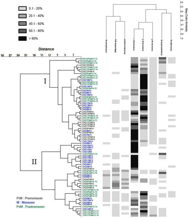
The respective abundances of each species across the study period have been compared from Figures 8–10. The total number of species observed during Monsoon'13 displayed an oscillating pattern with higher numbers (12 species) observed in July and September compared with August and October (five species). However, this pattern was absent in Monsoon'14 (Figure 8). During Post-Monsoon months from both 2013–2014 and 2014–2015 high numbers of species (10 species) were recorded (Figure 9). The calcareous genus, Ammonia was abundant throughout all the samples often constituting >80% of the total assemblage. It comprised three morphotypes, considered to represent three putatively distinct species based on observable morphological attributes. All three members of genus Ammonia had higher abundances during this time compared with Monsoon months (Figure 10). The porcelaneous Q. seminula displayed higher abundance in November 2013, while the agglutinated Miliammina spp. tests were constantly present across all eight months. In Pre-Monsoon season of 2014 a lesser number of species was encountered with maximum contribution from Ammonia spp., Q. seminula and Miliammina spp. In order to test whether the recorded foraminiferal assemblage was shaped by seasonal or spatial variation, species abundances across the 299 samples were regrouped into 75 seasonal groups (15 stations × 5 seasons) by calculating mean abundance of each species seasonally (Figure 13). The r-mode cluster analyses separated foraminiferal species having >10% relative abundance based on their occurrence in the sample.

Fig. 13. Hierarchical cluster analysis (Ward's method, Bray–Curtis similarity index) based on the species composition values regrouped seasonally; PrM, Pre-Monsoon; M, Monsoon; PsM, Post-Monsoon.
The agglutinated species of Ammodiscus sp., Miliammina spp. and Ammotium salsum clustered separately in Cluster II of the q-mode analyses that comprised mostly of stations CNS3–CNS6, CNS12, CNS14 and CNS17. Cluster I of the q-mode analyses however, comprised mostly samples with higher relative abundances of calcareous forms. Samples of Cluster I mostly originated from stations CNS7–11, CNS15 and CNS16. Seasonal clustering of samples was not observed in this study, indicating the absence of seasonal variability in benthic foraminiferal assemblages in Chilika lagoon.
The relationship between the observed assemblage diversity and measured environmental parameters was investigated by performing canonical correspondence analysis by considering absolute abundance data of the 13 species, Shannon Diversity index (H′), Species richness (S) and Log abundance as biotic variables. Figure 14 presents the result as a biplot where two axes cumulatively explained 78.84% of the observed variation within the data. Highly abundant and frequently occurring calcareous forms clustered separately from the less frequent agglutinated forms. Abundance of Ammonia sp.1, Ammonia sp.2 and Nonionella sp. showed a positive relationship with pH and dissolved NO3− concentrations and a negative relationship with TOC, salinity and depth. The relationships were reversed in the case of agglutinated species such as Trochammina inflata, A. salsum, Miliammina spp. and Ammodiscus sp. Overall species richness (S) and Shannon diversity (H′) also displayed a positive relationship with salinity, TOC, DO and depth. The porcelaneous species Q. seminula displayed a positive relation with silt clay content and a negative relation with dissolved silicate concentration.

Fig. 14. Canonical correspondence analysis of benthic foraminifera species with relation to the environmental parameters recorded for 20 months in Chilika lagoon.
The relationships observed in the CCA plot were cross-referenced by calculating the Pearson's correlation coefficient (r) values among biotic and abiotic variables observed throughout the study period (Table 3). Among all factors, only DO concentration and dissolved silicate concentration displayed significant (P < 0.05) positive correlations with both Shannon diversity (H′) and Margalef's species richness (S) and a negative correlation with total foraminiferal abundance. TOC and salinity showed significant negative and positive correlations respectively with richness; however, no such significant correlation was found in case of H′ and total abundance. Among the observed foraminiferal species, the most abundant species Ammonia sp.1 exhibited significant negative correlation with DO and dissolved silicate. The most abundant agglutinated genus Miliammina however exhibited positive correlation (0.18) with salinity. Miliammina and Ammodiscus both represented significant positive values of r with depth. TOC values showed a negative correlation with the abundant genus Ammonia represented by the three species while a strong positive correlation was observed with the porcelaneous species Quinqueloculina seminula.
Table 3. Pearson's correlation coefficient (r) between Margalef's richness (S), total abundance per 50 cm3 of sediment, Shannon diversity (H′), benthic foraminiferal species and physico-chemical parameters. Bold values indicate significant (P < 0.05) correlation.

DISCUSSION
Long-term monitoring approaches from coastal lagoons are largely limited. Previous examples of this approach have been undertaken from the Indian River lagoon in Florida (Buzas et al., Reference Buzas, Hayek, Reed and Jett2002) and Tees estuary in the UK (Horton & Murray, Reference Horton and Murray2007). In this respect, the present study is the first detailed long-term study from an Asian coastal lagoon. The contribution of taphonomically altered tests was pronounced in the stations with high abundance and in stations located in the Central sector of the lagoon. This information can provide insights regarding taphonomic alteration of assemblage structure and whether the source of taphonomic alteration originates from physical properties of the environment such as wave action or from chemical properties such as prevailing pH (Goldstein & Watkins, Reference Goldstein and Watkins1999; Walker & Goldstein, Reference Walker and Goldstein1999). In this study low foraminifera diversity (H′ = 0.3–0.95) was encountered inside the lagoon (Figure 11) as opposed to previous reports (Rao et al., Reference Rao, Jayalakshmy, Venugopal, Gopalakrishnan and Rajagopal2000). Compared with the global range of diversity values (H′ = 0.5–2.5) observed from lagoons and estuaries (Murray, Reference Murray2006) and from the recent work of Frontalini et al. (Reference Frontalini, Armynot du Châtelet, Debenay, Coccioni, Bancalà and Friedman2011), the present range is extremely low indicating the stressed nature of studied environment.
Benthic foraminiferal studies from the Chilika lagoon date back almost 50 years (Rajan, Reference Rajan1965); however none of the previous studies have looked at these sedimentary organisms on a seasonal scale. Additionally, many of these studies have focused mostly on the Outer channel compared with the Southern and Central sectors of the lagoon (e.g. Rao et al., Reference Rao, Jayalakshmy, Venugopal, Gopalakrishnan and Rajagopal2000; Kumar et al., Reference Kumar, Naidu and Kaladhar2015). The seasonal distribution pattern across the sampling months showed that benthic foraminiferal patterns between the same seasons of different years did not exhibit marked variation (Figures 8–10) whereas conserved assemblage patterns did exist spatially (Figure 12). The present study showed that taxonomic diversity of benthic foraminifera inside the Chilika lagoon is similar to previous reports from different lagoons globally. Frontalini et al. (Reference Frontalini, Coccioni and Bucci2010) studied the benthic foraminiferal assemblage from the lagoons of Orbetello and Lesina, Italy and found the presence of 13 species. Similar low diversity assemblage was noted from the lagoon in Venice (Coccioni et al., Reference Coccioni, Frontalini, Marsili and Mana2009) and Lake Varano in southern Italy (Frontalini et al., Reference Frontalini, Semprucci, Armynot du Châtelet, Francescangeli, Margeritelli, Rettori, Spagnoli, Balsamo and Coccioni2014), where Ammonia was found to be the most dominant genus. In Chilika, the existence of the genus Ammonia across all the stations demonstrates its stress-tolerant and cosmopolitan nature as also reported from other lagoonal environments (Coccioni et al., Reference Coccioni, Frontalini, Marsili and Mana2009; Frontalini et al., Reference Frontalini, Buosi, Da Pelo, Coccioni, Cherchi and Bucci2009). The Central sector of the lagoon showed the dominance of Ammonia spp. with relative abundance of more than 80% for Ammonia sp.1 and also a high value of occurrence (84%) (Figure 13). This could be attributed to the wide range of tolerance exhibited by members belonging to the genus Ammonia (Moodley & Hess, Reference Moodley and Hess1998; Le Cadre & Debenay, Reference Le Cadre and Debenay2006; Hallock, Reference Hallock2012). The Southern sector of the lagoon is marked by higher ranges of diversity and lower abundance as compared with the Central sector, which was also apparent from the separate clustering of stations based on q-mode cluster analysis (Figure 13). The Southern sector stations (CNS3–CNS6) clustered into Group I which corresponded to relatively high diversity and low abundance while Group II represented stations that showed low diversity and high abundance representing the Central sector. The relatively higher values of diversity observed in the Southern sector may be indicative of less-disturbed or pristine settings as high values of H′ (0.94 and 0.95) were observed in certain stations in this sector, which were totally devoid of any fishing activities and set-net operations. Agglutinated specimens belonging to A. salsum, Ammomarginulina sp., Ammodiscus sp. and Miliammina spp., typical of vegetated coastal environments (Berkeley et al., Reference Berkeley, Perry, Smithers, Horton and Taylor2007) constituted the majority of the assemblages in the Southern sector of the lagoon and also had higher relative abundance (>10%) compared with the Central sector (<1%). Although the frequency of occurrence (FO) of agglutinated species was low across all collected samples (Figure 12), they were more frequently recorded in the Southern sector and almost absent in stations in close proximity to the Northern sector of lagoon (CNS16 and CNS17). Chilika is a marginal coastal lagoonal environment which is heavily infested with weeds, similar to many global environments threatened with similar issues (Lloret et al., Reference Lloret, Marín and Marín-Guirao2008; Anthony et al., Reference Anthony, Atwood, August, Byron, Cobb, Foster, Fry, Gold, Hagos, Heffner and Kellogg2009). A significant seasonal difference in the concentration of dissolved nitrate (Figure 3) supports the idea that seasonal nutrient influx from adjoining regions is the major driving factor that shapes the lagoon environment. The seasonal variation observed in the prevailing environmental conditions did not appear to affect total foraminiferal assemblage of the lagoon. Seasonal changes in assemblage composition were virtually non-existent as revealed by the non-specific grouping of seasonal samples based on cluster analysis (Figure 13). The dissolved nutrient conditions as recorded in bottom water of the lagoon reflected signs of eutrophication characterized by episodic inputs that may be of natural or anthropogenic origin. Recent investigations have identified the lagoon to be clearly eutrophic to hyper-eutrophic with respect to its Trophic State Index (TSI) values calculated from light attenuation, Chlorophyll-a, total phosphate and total nitrate concentrations (Ganguly et al., Reference Ganguly, Patra, Muduli, Vardhan, Abhilash, Robin and Subramanian2015). Higher concentrations of TOC observed during and following monsoonal precipitation support the idea that increased production in the lagoon is supported by external nutrient influx (Figure 6). The benthic foraminiferal community however appeared to be unaffected by this change as the number of live specimens remained insignificant irrespective of the time of sampling.
Canonical correspondence analysis (CCA) of the observed variation in both biotic and environmental data provided key information regarding assemblage structure within the lagoon (Figure 14). The patchy occurrence of agglutinated species in the lagoon is explained in the CCA plot and correlation matrix by means of significant positive correlation of species A. salsum, Ammomarginulina sp., Ammodiscus sp. and Miliammina spp. with depth and salinity both being comparatively higher in this sector. The finding shows congruency with previous reports as most of the agglutinated foraminifera are known to be euryhaline (Sen Gupta et al., Reference Sen Gupta, Turner and Rabalais1996; Murray & Alve, Reference Murray and Alve2011). Although higher values of organic carbon (TOC) were observed in the Southern sector, no significant correlation of TOC was observed with respect to agglutinated species represented by A. salsum, Ammodiscus sp., Ammobaculites agglutinans, Textularia spp., T. inflata and Miliammina spp. The CCA plot only depicts the positive relation of TOC with agglutinated species along with positive correlation of depth and salinity. The presence of a positive relation indicates that the amount of food available to the sedimentary benthos apart from environmental conditions (such as salinity, depth and dissolved oxygen) influences the taxonomic composition of assemblages. Mojtahid et al. (Reference Mojtahid, Jorissen, Lansard, Fontanier, Bombled and Rabouille2009) while studying the organic matter enriched Rhne prodelta in the Mediterranean also noted similar dominance of stress-tolerant taxa in regions having higher organic matter content. The CCA plot showed a positive relation of sediment composition (silt/clay%) with Q. seminula while Ammomarginulina sp. displayed a significant positive correlation with the finer silt-clay fraction (<63 µm). Agglutinated foraminiferal species such as T. inflata and J. macrescens found in this study are known to preferentially select particles of certain size and mineralogy to construct their test irrespective of sediment composition (de Rijk & Troelstra, Reference de Rijk and Troelstra1999). The high FO (34%) and high relative abundance (<10%) of Miliammina spp. observed throughout the Chilika lagoon compared with other agglutinated opportunistic species such as T. inflata and J. macrescens, can be due to their tolerance to taphonomic effects and consequently better preservation potential (Berkeley et al., Reference Berkeley, Perry, Smithers, Horton and Taylor2007). Species belonging to the genus Miliammina are known to tolerate a wide range of salinity levels (1 to 35) and are thus regarded as euryhaline (Murray, Reference Murray1973, Reference Murray1983; Murray & Alve, Reference Murray and Alve2011). The relationship of Miliammina with depth in the present study is in line with previous reports where species of Miliammina have been reported to have an epiphytal mode of life and mostly restricted to marsh and shallow lagoon environments less than 2 m deep (Alve & Murray, Reference Alve and Murray1999; Murray, Reference Murray2006).
In the present study, the most dominant species, Ammonia sp.1, did not exhibit any significant correlation with any of the measured parameters except with dissolved oxygen (DO) and dissolved silicate concentration. The significant negative correlation with DO is consistent with the fact that members belonging to this genus are known to show high tolerance to hypoxic conditions (Kitazato, Reference Kitazato1994; Platon & Gupta, Reference Platon, Gupta, Rabalais and Turner2001). Low silicate values are known to correspond with high abundance of phytoplankton cells in Chilika that may in turn lead to increased phytodetrital input to sedimentary benthos (Srichandan et al., Reference Srichandan, Kim, Bhadury, Barik, Muduli, Samal, Pattnaik and Rastogi2015). Thus, the negative correlation of Ammonia with silicate indicates that dominance of this genus may increase under scenarios where primary production may be limited by its availability. The above finding further confirms the stress-tolerant nature of this genus. Previous studies have reported several species of Ammonia to be cosmopolitan with wide range of tolerance to salinity, pollution and organic matter (Debenay et al., Reference Debenay, Guillou, Redois, Geslin and Martin2000; Hayward et al., Reference Hayward, Holzmann, Grenfell, Pawlowski and Triggs2004; Carnahan et al., Reference Carnahan, Hoare, Hallock, Lidz and Reich2009). Alve (Reference Alve1995) noted that as organic contamination increases, population of tolerant species increases at the expense of more sensitive taxa (e.g. separate clustering of Group II in Figure 13 constituting the stations of the Central sector). In the present study it was observed that species of Ammonia showed higher abundance in stations of the Central sector with higher density of degraded tests indicating the episodic nature of anthropogenic pollution.
CONCLUSIONS
The benthic foraminiferal assemblage from Chilika lagoon was found to be temporally conserved as no significant seasonal variation was documented. The assemblage displayed spatial clustering with respect to diversity, abundance and assemblage composition. Members of the genus Ammonia were the most dominant component of the foraminifera assemblage and displayed no relationship with prevailing environmental conditions. However, total organic carbon, depth of the water column and salinity appeared to play a major role in controlling the agglutinated foraminiferal abundance. The data generated from the present study can be compared with similar environments globally in order to identify similar patterns and the role of environment towards shaping benthic organismal assemblages. Moreover, the generated data can also serve as a baseline for future palaeoenvironmental studies utilizing benthic foraminifera as a proxy.
SYSTEMATICS
Phylum FORAMINIFERA Margulis & Schwartz, 1998 Class TUBOTHALAMEA Pawlowski et al., 2013 Order MILIOLIDA Delage & Herouard, 1896 Family MILIAMMINIDAE Saidova, 1981 Genus Miliammina Heron-Allen & Earland, 1930 Miliammina fusca Brady, 1870 (Plate 2–1a, b) Miliammina obliqua Heron-Allen & Earland, 1930 (Plate 2–5a, b) Family HAUERINIDAE Schwager, 1876 Genus Quinqueloculina d'Orbigny, 1826 Quinqueloculina seminula Linnaeus, 1758 (Plate 2–4) Order SPIRILLINIDA Hohenegger & Piller, 1975 Family AMMODISCIDAE Reuss, 1862 Genus Ammodiscus Reuss, 1862 (Plate 2-2) Class GLOBOTHALAMEA Pawlowski et al., 2013 Subclass TEXTULARIIA Mikhalevich, 1980 Order LITUOLIDA Lankester, 1885 Family LITUOLIDAE Blainville, 1827 Genus Ammobaculites Cushman, 1910 Ammobaculites agglutinans d'Orbigny, 1826 (Plate 1–7) Genus Ammotium Loeblich & Tappan, 1953 Ammotium salsum Cushman & Broennimann, 1948 (Plate 1–8) Genus Ammomarginulina Wiesner, 1931 (Plate 1–9) Superfamily TROCHAMINOIDEA Schwager, 1877 Family TROCHAMMINIDAE Schwager, 1877 Genus Jadammina Bartenstein & Brand, 1938 Jadammina macrescens Brady, 1870 (Plate 1–10) Genus Trochammina Parker & Jones, 1859 Trochammina inflata Montagu, 1808 (Plate 1–4a, b) Order TEXTULARIIDA Superfamily TEXTULARIOIDEA Ehrenberg, 1838 Family TEXTULARIIDAE Ehrenberg, 1838 Genus Textularia Defrance, 1824 Textularia earlandii Parker, 1952 (Plate 2–5) Textularia agglutinans d'Orbigny, 1839 (Plate 2–6) Order ROTALIIDA Delage & Herouard, 1896 Superfamily ROTALIOIDEA Ehrenberg, 1839 Family AMMONIIDAE Saidova, 1981 Genus AMMONIA Brünnich, 1772 (Plate 1–3) Ammonia sp.1 cf. Ammonia T2: Hayward et al., Reference Hayward, Holzmann, Grenfell, Pawlowski and Triggs2004
DIAGNOSIS
Ammonia sp.1 is characterized by the presence of single small umbonal boss and 8 to 12 chambers in the final whorl (Plate 1-1a, b).
Ammonia sp.2 cf. Ammonia T6: Hayward et al., Reference Hayward, Holzmann, Grenfell, Pawlowski and Triggs2004
DIAGNOSIS
Ammonia sp. 2 is characterized by absence of umbonal boss and 6 to 8 chambers in the final whorl (Plate 1–2a, b).
Ammonia sp.3 cf. Ammonia T10: Hayward et al., Reference Hayward, Holzmann, Grenfell, Pawlowski and Triggs2004
DIAGNOSIS
Ammonia sp.3 is characterized by large globular chambers of 5 to 7 in final whorl (Plate 1–3).
Family NONIONIDAE Schultze, 1854 Genus Nonionella Rhumbler, 1949 (Plate 2–3)
ACKNOWLEDGEMENTS
The authors are grateful to Integrative Taxonomy and Microbial Ecology Research group members for helping during fieldwork. The authors would also like to acknowledge the assistance provided by Kashinath Sahoo during FESEM imaging of foraminiferal samples.
FINANCIAL SUPPORT
This work is supported by grants awarded to Punyasloke Bhadury by Chilika Development Authority through the financial support received from the World Bank supported Integrated Coastal Zone Management Project component of Odisha. Areen Sen acknowledges IISER Kolkata for the provision of a PhD Fellowship.