INTRODUCTION
The cetacean communities inhabiting tropical waters have been relatively well-studied in areas such as the Gulf of Mexico (e.g. Davis et al., Reference Davis, Fargion, May, Leming, Baumgartner, Evans, Hansen and Mullin1998, Reference Davis, Ortega-Ortiz, Ribic, Evans, Biggs, Ressler, Cady, Leben, Mullin and Würsig2002; Baumgartner et al., Reference Baumgartner, Mullin, May and Leming2001; Maze-Foley & Mullin, Reference Maze-Foley and Mullin2006), the Bahamas (e.g. MacLeod et al., Reference MacLeod, Hauser and Peckham2004), the eastern tropical Pacific Ocean (e.g. Au & Perryman, Reference Au and Perryman1985; Reilly, Reference Reilly1990; Ballance et al., Reference Ballance, Pitman and Fiedler2006) and the Indian Ocean (e.g. Ballance & Pitman, Reference Ballance and Pitman1998; Anderson, Reference Anderson2005; Gross et al., Reference Gross, Kiszka, Van Canneyt, Richard and Ridoux2009). Tropical cetacean communities are usually dominated by resident odontocete species that rely on the wider region to provide calving habitat and prey throughout the year. These typically include species such as Stenella and Delphinus dolphins, bottlenose dolphins (Tursiops spp.), rough-toothed dolphin (Steno bredanensis), Risso's dolphin (Grampus griseus), melon-headed whale (Peponocephala electra), false killer whale (Pseudorca crassidens), short-finned pilot whale (Globicephala macrorhynchus), Kogia species, beaked whales (family Ziphiidae) and the sperm whale (Physeter macrocephalus). Tropical cetacean communities also include seasonal residents that utilize tropical waters for part of the year, and migrant species that simply transit through the region. For example, the humpback whale (Megaptera novaeangliae) may both migrate through some tropical areas and seasonally occupy some as breeding grounds (Clapham & Mead, Reference Clapham and Mead1999), while the blue whale (Balaenoptera musculus) may breed seasonally and probably also forages within certain tropical areas (Ballance & Pitman, Reference Ballance and Pitman1998; Ballance et al., Reference Ballance, Pitman and Fiedler2006). The use of tropical waters as habitat may, therefore, vary between species depending on life-cycle stage and behavioural context.
In tropical waters, the distribution of top predators such as cetaceans tends to be patchy (Forney, Reference Forney2000; Yen et al., Reference Yen, Sydeman and Hyrenbach2004; Ballance et al., Reference Ballance, Pitman and Fiedler2006), relating to variation in the distribution of their prey (primarily epipelagic and mesopelagic fish and cephalopod species; Pauly et al., Reference Pauly, Trites, Capuli and Christensen1998). As a result, in most cases, the relationship of resident cetaceans with topographic and oceanographic habitat parameters is thought to be an indirect consequence of the relationships between cetacean prey and such variables (e.g. Selzer & Payne, Reference Selzer and Payne1988; Cañadas et al., Reference Cañadas, Sagarminaga and García-Tiscar2002; Davis et al., Reference Davis, Ortega-Ortiz, Ribic, Evans, Biggs, Ressler, Cady, Leben, Mullin and Würsig2002; Ballance et al., Reference Ballance, Pitman and Fiedler2006; Doksæter et al., Reference Doksæter, Olsen, Nøttestad and Fernö2008; Torres et al., Reference Torres, Read and Halpin2008). Neritic and oceanic communities of cetaceans have been described in many tropical areas (e.g. Davis et al., Reference Davis, Fargion, May, Leming, Baumgartner, Evans, Hansen and Mullin1998, Reference Davis, Ortega-Ortiz, Ribic, Evans, Biggs, Ressler, Cady, Leben, Mullin and Würsig2002; Baumgartner et al., Reference Baumgartner, Mullin, May and Leming2001; Hamazaki, Reference Hamazaki2002; Anderson, Reference Anderson2005; Maze-Foley & Mullin, Reference Maze-Foley and Mullin2006; Gannier, Reference Gannier2009), although the exact species composition of each community may vary between regions. For example, Atlantic spotted dolphins (Stenella frontalis) most often occur in continental shelf waters in the Gulf of Mexico (Griffin & Griffin, Reference Griffin and Griffin2003; Mullin & Fulling, Reference Mullin and Fulling2004), but predominantly inhabit oceanic waters off Angola (Weir, Reference Weir2007, Reference Weir2011). In addition to depth, the distribution of cetaceans has been related to topographic features such as seabed gradient (e.g. Baumgartner, Reference Baumgartner1997; Baumgartner et al., Reference Baumgartner, Mullin, May and Leming2001; Waring et al., Reference Waring, Hamazaki, Sheehan, Wood and Baker2001; Cañadas et al., Reference Cañadas, Sagarminaga and García-Tiscar2002; Azzellino et al., Reference Azzellino, Gaspari, Airoldi and Nani2008a; Doksæter et al., Reference Doksæter, Olsen, Nøttestad and Fernö2008), seabed aspect (e.g. MacLeod & Zuur, Reference MacLeod and Zuur2005) and high seabed relief (e.g. Hui, Reference Hui1979; Selzer & Payne, Reference Selzer and Payne1988). Topographic features may result in upwelling, turbulence and aggregation of prey species. Consequently the relationship between cetaceans and these features may be the result of interactions between topographic and local oceanographic factors rather than due to topography alone (Baumgartner, Reference Baumgartner1997; MacLeod & Zuur, Reference MacLeod and Zuur2005).
The oceanographic factors influencing the distribution of cetaceans are more complex to analyse and are often interlinked with one another, and with topographic factors. Oceanic marine environments are dynamic and experience considerable variation. For example, they may be influenced both spatially and temporally by surface- and deep-water currents, eddies, fronts, freshwater influxes from rivers and climatic phenomena such as the El Niño-Southern Oscillation and the North Atlantic Oscillation. Despite this complexity, relationships have been found between cetaceans and a number of oceanographic variables, including sea surface temperature (SST) (e.g. Au & Perryman, Reference Au and Perryman1985; Selzer & Payne, Reference Selzer and Payne1988; Waring et al., Reference Waring, Hamazaki, Sheehan, Wood and Baker2001; Hamazaki, Reference Hamazaki2002; Azzellino et al., Reference Azzellino, Gaspari, Airoldi and Lanfredi2008b; Doksæter et al., Reference Doksæter, Olsen, Nøttestad and Fernö2008), SST variability (e.g. Davis et al., Reference Davis, Fargion, May, Leming, Baumgartner, Evans, Hansen and Mullin1998; Baumgartner et al., Reference Baumgartner, Mullin, May and Leming2001), surface chlorophyll concentrations (e.g. Smith et al., Reference Smith, Dustan, Au, Baker and Dunlap1986; Jaquet et al., Reference Jaquet, Whitehead and Lewis1996), turbidity (e.g. Bräger et al., Reference Bräger, Harraway and Manly2003), salinity (e.g. Selzer & Payne, Reference Selzer and Payne1988; Griffin & Griffin, Reference Griffin and Griffin2003; Doksæter et al., Reference Doksæter, Olsen, Nøttestad and Fernö2008) and thermocline depth (e.g. Reilly, Reference Reilly1990; Reilly & Fiedler, Reference Reilly and Fiedler1994; Ballance et al., Reference Ballance, Pitman and Fiedler2006).
The distribution of a cetacean species in relation to topographic and oceanographic variables will be defined, at least in part, by the ecological niche that the species occupies within a specific region. The ecological niche concept was formalized by Hutchinson (Reference Hutchinson1958) who described a species' fundamental niche as an n-dimensional hypervolume that encloses all possible combinations of values for n limiting niche factors where a species can persist. However, since similar species may compete for the same resources, the realized niche is often smaller than the fundamental niche. In addition, the unique historical characteristics of individual species may mean that they do not occur in specific areas of otherwise suitable habitat. Resident odontocete communities often consist of several ecologically and/or taxonomically similar cetacean species. For example, multiple species of Stenella and/or Delphinus dolphins have been recorded in many tropical communities studied to date (e.g. Au & Perryman, Reference Au and Perryman1985; Reilly & Fiedler, Reference Reilly and Fiedler1994; Davis et al., Reference Davis, Fargion, May, Leming, Baumgartner, Evans, Hansen and Mullin1998, Reference Davis, Ortega-Ortiz, Ribic, Evans, Biggs, Ressler, Cady, Leben, Mullin and Würsig2002; Anderson, Reference Anderson2005; Ballance et al., Reference Ballance, Pitman and Fiedler2006; Maze-Foley & Mullin, Reference Maze-Foley and Mullin2006; Gannier, Reference Gannier2009; Gross et al., Reference Gross, Kiszka, Van Canneyt, Richard and Ridoux2009). Consequently, it might be expected that competition between sympatric and ecologically-similar cetacean species may lead to partitioning of resources via factors such as spatial and temporal segregation (e.g. differential habitat use related to water depth, seabed slope and productivity, variation in relative foraging depth and diurnal feeding pattern) and differences in prey preferences (e.g. prey species and prey size) (Bearzi, Reference Bearzi2005).
There are many instances of habitat partitioning between sympatric cetacean species described within the scientific literature. For example, habitat partitioning occurs in relation to SST and salinity between Atlantic white-sided dolphins (Lagenorhynchus acutus) and short-beaked common dolphins (Delphinus delphis) off the north-eastern USA (Selzer & Payne, Reference Selzer and Payne1988), by SST between Physeter macrocephalus and beaked whales off the north-eastern USA (Waring et al., Reference Waring, Hamazaki, Sheehan, Wood and Baker2001), by depth, distance from shore and salinity between common bottlenose dolphins (Tursiops truncatus) and Stenella frontalis in the Gulf of Mexico (Griffin & Griffin, Reference Griffin and Griffin2003), by water depth and diet between T. truncatus and the pantropical spotted dolphin (S. attenuata) in Golfo Dulce, Costa Rica (Oviedo, Reference Oviedo2007), by depth and distance from shore between T. truncatus, Steno bredanensis and Guiana dolphins (Sotalia guianensis) at Abrolhos Bank, Brazil (Rossi-Santos et al., Reference Rossi-Santos, Wedekin and Sousa-Lima2006), by depth and slope between Grampus griseus and Cuvier's beaked whales (Ziphius cavirostris) in the Ligurian Sea (Azzellino et al., Reference Azzellino, Gaspari, Airoldi and Nani2008a), by SST between the white-beaked dolphin (Lagenorhynchus albirostris) and D. delphis in UK shelf waters (MacLeod et al., Reference MacLeod, Weir, Santos and Dunn2008), and by depth and diet between the Indo-Pacific bottlenose dolphin (T. aduncus), S. attenuata, spinner dolphins (Stenella longirostris) and Peponocephala electra around Mayotte in the south-west Indian Ocean (Gross et al., Reference Gross, Kiszka, Van Canneyt, Richard and Ridoux2009).
This study used data collected from non-dedicated platforms to compare the habitat preferences of cetacean species observed in the tropical waters located between Angola and Gabon in the eastern tropical Atlantic between 2004 and 2009. Studies of the cetacean community occupying this area, particularly in offshore waters, commenced relatively recently (Weir, Reference Weir2007), and very little is known about their ecology and relationships with their environment. The use of non-dedicated platforms is cost-effective and, in some poorly-known and inaccessible areas (including the study area), represents the only currently available means of gathering data on oceanic cetaceans. However, their use is subject to limitations, particularly the lack of control over the areas and habitats surveyed (Evans & Hammond, Reference Evans and Hammond2004; Redfern et al., Reference Redfern, Ferguson, Becker, Hyrenbach, Good, Barlow, Kaschner, Baumgartner, Forney, Ballance, Fauchald, Halpin, Hamazaki, Pershing, Qian, Read, Reilly, Torres and Werner2006). In addition, the data presented here were not specifically collected to investigate the relationship between cetaceans and their habitat. Nevertheless, it is of interest and conservation relevance to determine whether inferences on the habitat preferences exhibited by cetacean species in a region can be made using such data, when no other information is available.
The dataset was analysed with the following objectives: (1) to describe the habitat preferences of the eight cetacean species inhabiting a region of the eastern tropical Atlantic throughout the year (i.e. ‘residents’) in terms of the habitats surveyed; (2) to investigate the extent to which eight species partition their habitat niche in relation to four ecogeographical variables; and (3) to develop a novel approach for comparing the niches occupied by cetacean species within a specific area of interest using an opportunistic dataset.
MATERIALS AND METHODS
The study area
The study area extended from Gabon to Angola in the eastern tropical Atlantic Ocean, spanning latitudes from 1°N to 11°S (Figure 1). The region is characterized by a continental shelf of less than 70 km width in most places, with water depth increasing to over 5000 m in the Angola Basin. The oceanography of the northern part of the study area is dominated by the warm water Guinea Current which flows southwards along the coast of Gabon where it turns offshore and moves westwards as the South Equatorial Current (Longhurst, Reference Longhurst1962). A nutrient-poor, warm water (>24°C) current, the Angola Current, continues southwards over Angolan shelf and shelf-edge waters before converging with the cooler-water northward-flowing Benguela Current at the Angola–Benguela frontal zone (Hardman-Mountford et al., Reference Hardman-Mountford, Richardson, Agenbag, Hagen, Nykjaer, Shillington and Villacastin2003). The front exists as a permanent year-round oceanographic feature in a latitudinal band between 14°S and 16°S (Hardman-Mountford et al., Reference Hardman-Mountford, Richardson, Agenbag, Hagen, Nykjaer, Shillington and Villacastin2003). The 11°S southern limit of the study area ensured that habitat preferences were compared amongst an exclusively tropical (≥20°C surface temperature) cetacean community (i.e. well north of the main Angola–Benguela frontal zone). The Congo River is the largest freshwater input to any worldwide eastern ocean boundary (Hardman-Mountford et al., Reference Hardman-Mountford, Richardson, Agenbag, Hagen, Nykjaer, Shillington and Villacastin2003), and causes peaks in primary productivity around 150–200 km from the river mouth in the waters off the Democratic Republic of the Congo and Angola (van Bennekom & Berger, Reference van Bennekom and Berger1984). As a result of this spatial variation in water temperature, currents, frontal systems and freshwater input, the study area includes a variety of potential cetacean habitats.

Fig. 1. Location of the study area and occupied 10 × 10 km grid cells in the eastern tropical Atlantic: (A) all cetacean-occupied cells (N = 550; 251 of these cells were occupied by cetaceans in more than one month/year) used in the principal component analysis; (B) Balaenoptera brydei; (C) Physeter macrocephalus; and (D) Delphinus sp.
Cetacean data
A total of 3323 cetacean sightings was collected from non-dedicated platforms operating within the study area. A subset of 2873 sightings (Table 1) was selected for analysis based on the following criteria: (1) sightings were recorded between 1°N and 11°S latitude, and between January 2004 and June 2009; (2) there was high confidence in the species identification; (3) there was an accurate GPS position; (4) sightings were ≤10 km distance from the survey platform; and (5) sightings had all relevant associated information (month, year and all environmental variables—see below).
Table 1. Total cetacean sightings (N = 2873) selected for analysis and the number of 10 × 10 km grid cells available for each species for the principal component analysis (PCA). Of the year-round species, only species 1–8 had sufficient sample size (≥30 grid cells) for niche analysis. Species 9–21 were used in the PCA and to produce absence cells for the classification tree (CT) analysis. Unidentified categories 22 and 23 were used in the PCA, and to produce absence cells for CT analysis for whales and delphinids respectively. Unidentified category 24 was used in the PCA only.

The majority of records (N = 2852; 99.3%) originated from eight experienced observers working on-board geophysical survey vessels. The emission of airgun sound during geophysical surveys may potentially influence cetaceans through factors such as masking of their communication and navigation signals, altered behaviour, temporary or permanent hearing/tissue damage, stress or displacement from habitat (Richardson et al., Reference Richardson, Greene, Malme and Thomson1995; Nowacek et al., Reference Nowacek, Thorne, Johnston and Tyack2007). However, while acknowledging that the datasets collected from geophysical survey vessels are potentially influenced by unknown reactions of cetacean species to airgun sound, such vessels can serve as non-dedicated research platforms from which to document cetacean communities within poorly-surveyed regions (e.g. Weir, Reference Weir2007, Reference Weir2011; de Boer, Reference de Boer2010). Briefly (see Weir, Reference Weir2007 and Weir, Reference Weir2011 for further details of the methodology), a single dedicated observer maintained a watch for cetaceans throughout daylight hours (with adequate breaks to maintain concentration), scanning the 180° area from beam to beam ahead of the ship (with regular 360° scans) using the unaided eye and 8–10× binoculars. The height of the observation platform on-board the vessels ranged from 10.5 to 20.5 m above sea level. Vessel speed was predominantly 4–5 knots (or 8 km h−1), with around 3% of total effort occurring during transits at speeds ranging from 7 to 12 knots (13–22 km h−1) (Weir, Reference Weir2011). Whenever a cetacean individual or group (i.e. a ‘sighting’) was observed, data including the species, position, distance from the vessel (estimated using naked eye or calculated with a range stick or the vessel's radar) and water depth were recorded.
A further 21 sightings were included in the analysis, comprising: (1) 12 sightings from a sports fishing vessel operating from Luanda where photographs were provided to verify the species; and (2) nine sightings (mostly unidentified dolphins) from crew members on-board seismic or support vessels where sightings were verified based on descriptions.
Method selection criteria
The data collected during the surveys were subject to a number of caveats that restricted the use of more traditional methods of cetacean–habitat analysis (see Redfern et al., Reference Redfern, Ferguson, Becker, Hyrenbach, Good, Barlow, Kaschner, Baumgartner, Forney, Ballance, Fauchald, Halpin, Hamazaki, Pershing, Qian, Read, Reilly, Torres and Werner2006), and these are outlined here.
Firstly, although associated effort data were collected for many of the sightings, the effort data were not suitable for providing accurate habitat absence information because of limitations resulting from the use of geophysical platforms. In particular, a recorded absence of animals from a geophysical platform might potentially reflect a response of animals to seismic operations rather than representing unsuitable habitat.
It is of course always the case that absence of a cetacean species from a particular location during one or more surveys does not necessarily indicate unsuitable habitat, and the likelihood of it being a true absence increases the more times the location is surveyed. Absence records recorded from geophysical platforms may be particularly unreliable as indications of unsuitable habitat. However, it is reasonably certain that the location where a species was recorded reflects habitat where they do occur, and these datasets can, therefore, provide information on species occurrence.
Secondly, high resolution geophysical surveys typically travel along transects at a spacing of 25 m, resulting in repeated transits across the same area during consecutive weeks. Consequently, there is potential for repeated encounters with the same animals at the same location. As these would not represent separate habitat selection events by cetaceans, they cannot necessarily be considered as independent data points (thus violating the requirements for independence required by many statistical tests; Redfern et al., Reference Redfern, Ferguson, Becker, Hyrenbach, Good, Barlow, Kaschner, Baumgartner, Forney, Ballance, Fauchald, Halpin, Hamazaki, Pershing, Qian, Read, Reilly, Torres and Werner2006). In addition, for some social cetacean species (particularly Physeter macrocephalus) it is sometimes problematic to determine what represents a group, and consequently which sightings represent independent samples.
Both of these potential issues were minimized by adopting a grid cell structure where occurrence in a grid cell per survey month per year by each species was used as the unit for statistical analysis. Consequently, multiple sightings that occurred closely in space or time for reasons which do not represent separate habitat selection events would not be counted repeatedly as independent data points, but rather would be analysed as a single point.
Precise distance and bearing measurements were not always available to calculate the actual position of a sighting and link it to location-specific environmental variables. The ship's position was therefore used as an approximation of the actual position of each sighting. A 10 × 10 km grid cell resolution was used, since 10 km was the maximum distance between the ship and most observed cetaceans and is also an appropriate scale to represent mesoscale oceanographic features such as fronts and eddies (Redfern et al., Reference Redfern, Ferguson, Becker, Hyrenbach, Good, Barlow, Kaschner, Baumgartner, Forney, Ballance, Fauchald, Halpin, Hamazaki, Pershing, Qian, Read, Reilly, Torres and Werner2006). Some sightings will inevitably fall outside of the assigned grid cell. However, none will be further away than the immediate neighbouring grid cell, which should have approximately similar ecogeographical variables (EGVs). The data were re-analysed using 20 × 20 km grid cells in order to investigate the potential impacts of scale on the relationship of cetaceans with their habitat. However, the principal component analysis (PCA) results were very similar to those for the 10 × 10 km dataset, and since the sample size was much smaller using the 20 km resolution, only results from the 10 km resolution dataset are presented here.
Ecogeographical variables
Cetacean sighting data were entered into a Geographic Information System (GIS) created in Environmental Systems Research Institute (ESRI) ArcView 3.2 software. The selection of the habitat variables used in the study was based on the oceanography of the study area, information on the key factors governing the same (or similar) species elsewhere, and the availability of data. Four EGVs were chosen, comprising two topographical and two oceanographic variables.
The two topographic variables were water depth and seabed slope. The relationship between cetacean distribution and seabed topography is typically determined by relatively fine-scale topographic variation. Therefore, water depths were obtained from the GEBCO Digital Atlas 2003 and converted into a 1 km2 grid, from which a grid of seabed slope was derived using ArcView functions. The average depth (m) and slope (degrees) for all 1 km2 cells was then calculated and used as an index of depth and slope for each 10 × 10 km resolution cell where cetaceans were recorded.
Data on two oceanographic variables, sea surface temperature (SST) and oceanic front probability were available. SST was provided as 4.6 km resolution monthly composites from the Moderate Resolution Imaging Spectroradiometer (MODIS) on the NASA Aqua satellite (provided by NEODAAS, Plymouth Marine Laboratory). Monthly composite front maps (4.6 km resolution), derived from SST and ocean colour data originating from the NASA MODIS instrument, were provided by NEODAAS. The front maps were based on: (1) the strength and persistence of frontal systems within the study area as determined using the temporal persistence of frontal features (probability of observing a front at a particular pixel within that month); and (2) the front's SST gradient strength (K/pixel) (Fpersist maps: Miller, Reference Miller2004, Reference Miller2009). The maps summarize sequences of partially cloud-covered scenes without blurring dynamic fronts (Miller, Reference Miller2004). A Gaussian smoothing filter of width σ = 15 pixels was applied to blur the individual front observations into single monthly composites of relative front strength (FS). Data for a third potential EGV provided by MODIS, chlorophyll-α, were initially examined but coverage was very poor due to cloud cover and these data were consequently not included further.
The average values of SST and FS per 10 × 10 km cetacean sampling grid cell were extracted for each of the 53 survey months in the January 2004 to June 2009 period during which cetaceans were recorded.
Statistical analysis
SELECTION OF CETACEAN SPECIES
Statistical analysis was carried out on eight cetacean species that were year-round residents within the study area (Weir, Reference Weir2011), and that had an adequate sample size defined as ≥30 grid cells (Hamazaki, Reference Hamazaki2002). Megaptera novaeangliae was excluded because although the sample size for this species was adequate, their occurrence in the study area is strongly seasonal (Weir, Reference Weir2011) and many whales migrate through the study area to calving/breeding areas further north and west in the Gulf of Guinea region. Consequently, there is a high likelihood that M. novaeangliae are merely transiting through the region rather than these areas representing key niche habitat.
HABITAT PREFERENCE ANALYSIS
The habitat preferences (within those habitats surveyed) of the eight species were firstly compared using classification trees (CTs) (Breiman et al., Reference Breiman, Friedman, Olshen and Stone1984). This method is used to explore the relationship between a single response variable (presence or absence of the species) and several explanatory variables (the four EGVs). Any grid cell where a species was recorded was considered a presence data point in this analysis. The monthly grid cells where other positively-identified species were recorded, but not the species being investigated, were used to indicate locations which were sampled but where the target species was absent. Since large whales (baleen and sperm whales) are very visually distinguishable from schools of delphinids at sea, grid cells occupied by unidentified large whales but not by the species being investigated were used as absence data for Globicephala macrorhynchus, Grampus griseus, Tursiops truncatus, Stenella frontalis, S. coeruleoalba and Delphinus sp. (total presence/absence grid cells = 782). Similarly, grid cells occupied by unidentified dolphins but not by the species being investigated were used as absence data for Bryde's whale (Balaenoptera brydei) and Physeter macrocephalus (total presence/absence grid cells = 1038). While this type of absence data cannot provide information about the absolute habitat preferences of a species, they can provide a measure of its habitat preferences relative to the other species recorded in the study area (MacLeod et al., Reference MacLeod, Weir, Pierpoint and Harland2007).
Classification trees were used to compare whether the niche occupied by each of the eight cetacean species differed from the general cetacean niche, in terms of the EGVs and the habitat combinations sampled. The CTs were constructed using BRODGAR software (available from www.highstat.com) as an interface for R statistical software. CTs split the total (i.e. root) presence/absence dataset into two subsets (i.e. branches) based on the value of a single EGV which maximizes between-group variance. The resulting branches are then repeatedly split into two subsets to produce a hierarchical tree of nodes, with each successive split determined by the key value of the most important EGV. To ensure that trees were simple and robust, branching was constrained according to the following criteria: (1) splitting of a branch only occurred if the branch comprised ≥30 presence–absence data points; (2) following the initial split, subsequent splits were made only when species presence accounted for ≥20% of the total data points within one of the resulting branches (indicating that the EGV was a major explanatory influence for the species); and (3) when a tree had multiple branches fulfilling the first and second criteria, it was manually pruned such that only the first four splits were presented, in order to identify the most important EGVs.
COMPARISON OF THE NICHES OCCUPIED BY INDIVIDUAL SPECIES
While CTs provide information on the habitat preferences of individual species, they do not necessarily allow the niches occupied by individual species to be compared. Therefore, in order to specifically compare the habitat niches occupied by different cetacean species, a PCA was carried out on the EGVs using Minitab statistical software (Minitab Ltd). PCA takes advantage of collinearity between the EGVs to generate new, independent, synthetic axes, such that the majority of the variation in the original set of EGVs is captured in a smaller number of axes (i.e. it reduces the dimensionality of multivariate data) (Redfern et al., Reference Redfern, Ferguson, Becker, Hyrenbach, Good, Barlow, Kaschner, Baumgartner, Forney, Ballance, Fauchald, Halpin, Hamazaki, Pershing, Qian, Read, Reilly, Torres and Werner2006). In the present context, the approach is useful if the first few PCA axes account for a substantial proportion of variation in the original data. The PCA was carried out on a database containing each cetacean-occupied (including all species and unidentified cetaceans; Table 1) grid cell per survey month per year (N = 1087), to describe an overall cetacean niche. Since the four EGVs had different units, these data were standardized prior to the PCA by subtracting the mean value from the actual value and dividing by the standard deviation.
Statistical tests were then carried out in Minitab to examine differences in the distribution of grid cells occupied by the eight individual cetacean species along the independent axes (based on the EGVs) generated from the PCA. Specifically, two components of this distribution were compared. These were: (1) the median value, which is an indicator of the niche centre occupied along a specific principal component (PC) axis in relation to the other species recorded and the locations sampled; and (2) the variance in PC scores, which is an indicator of the niche width occupied by a species along a specific PC axis. Again, this does not provide a measure of the absolute niche overlap between each species. Instead, it provides a measure of how the species overlap within the areas where cetaceans were recorded during this study.
The species PC scores were compared using Kruskal–Wallis tests carried out on each PC axis separately, to examine whether cetacean species could be differentiated with respect to habitat variables. If there was a significant difference (indicating a difference in median PC score between at least two species), pairwise comparisons were carried out using Mann–Whitney U-tests to assess which species pairs were responsible for the difference. F tests (first axis) for normally-distributed datasets, or Levene's tests (second and third axes) for non-normal datasets, were used to examine whether the PC scores for each pair of species had significantly different variance, indicating that they differed in terms of the relative width of the niche occupied. The first three axes were analysed in turn with the aim of identifying the most important axis (if any) that produced a significant difference in niche centre and width for each species pair.
While these pairwise comparisons could be considered as separate tests investigating different research questions (i.e. what is the difference in niche characteristics between a specific pair of species?), it could also be argued that they are multiple tests to investigate the same research question (i.e. are there niche differences between any species in the study area?). Therefore, a Bonferroni correction was applied to reduce risk of a type II statistical error and identify a more appropriate threshold for significance. The typical 0.05 probability threshold for statistical significance was divided by the number of pairwise comparisons being carried out.
RESULTS
Cetacean-occupied grid cells were widely distributed across the study area, but were concentrated in the waters off northern Angola and the Democratic Republic of the Congo (Figure 1A), where the bulk of survey effort occurred (see Weir, Reference Weir2011). Eight resident species were recorded in ≥30 grid cells and were used in the habitat preference analyses, with Physeter macrocephalus and Globicephala macrorhynchus recorded in the highest number of grid cells (Table 1). The distributions of grid cells for Balaenoptera brydei, P. macrocephalus and Delphinus sp. are illustrated in Figure 1B–D.
Habitat preference analysis
For most of the species, SST (Balaenoptera brydei, Physeter macrocephalus, Globicephala macrorhynchus and Delphinus sp.) or water depth (Grampus griseus, Tursiops truncatus and Stenella frontalis) was the most important EGV (of those examined) relating to species presence relative to other cetaceans (Figure 2). SST was the most important EGV determining the presence of B. brydei (Figure 2A), with a preference for waters cooler than 20.6°C. In warmer water areas seabed slope was important, with a preference for slope steeper than 1.77°. SST was also the most important EGV relating to P. macrocephalus presence, with a preference for SSTs greater than 23.6°C and water depths exceeding 1055 m (Figure 2B). The presence of G. macrorhynchus was most strongly explained by SSTs higher than 25.3°C, after which water depth became important with presence more likely in depths shallower than 1500 m (Figure 2C).

Fig. 2. Classification trees showing the habitat preferences of eight cetacean species in the eastern tropical Atlantic: (A) Balaenoptera brydei; (B) Physeter macrocephalus; (C) Globicephala macrorhynchus; (D) Grampus griseus; (E) Tursiops truncatus; (F) Stenella frontalis; (G) Stenella coeruleoalba; (H) Delphinus sp. Percentages refer to the proportion of data points (absence and presence data points combined: n) within a branch that comprises the species.
The separation of Grampus griseus, Tursiops truncatus, Stenella frontalis and S. coeruleoalba from other locations where cetaceans were recorded was relatively poor using the CT method, as indicated by the simple structure of the trees for these species (Figure 2D–G). In these cases, the initial split resulted in branches where species presence accounted for <20% of the total data points in each branch, and consequently no further splits were made. The presence of three of these species was primarily explained by water depth. Grampus griseus was more likely to be present in depths of less then 1669 m (Figure 2D), T. truncatus was more likely to be present in depths of less than 1725 m (Figure 2E) and S. frontalis was most likely to be present at depths of less than 1616 m (Figure 2F). For Stenella coeruleoalba, seabed slope was the most important EGV, with a higher presence in areas where the seabed slope was greater than 0.635° (Figure 2G).
Sea surface temperature was the most important EGV describing Delphinus sp. presence (Figure 2H), with higher presence at SSTs lower than 22.1°C. Within cooler waters FS was also important, with a higher occurrence at FS greater than 16.5. Therefore, within the range examined, Delphinus sp. preferred cooler waters and areas of high frontal strength.
Comparison of the niches occupied by individual species
The first three principal components (PC1–PC3) explained over 80% of dataset variance (Table 2). Axis 1 accounted for the first 31% of variation (Table 2). Only species pairs that were not significantly different on the first axis were compared on the second axis, and similarly with the third axis, with the aim of identifying the most important axis describing niche differences between each species pair. Results of all comparisons are shown in Table 3.
Table 2. Results of the principal component analysis (PCA) carried out on the four standardized ecogeographical variables for cetacean-positive grid cells (N = 1087). The first three axes account for ~85% of the variation. The most important variable on each principal component (PC) axis is shown in bold.

Table 3. Pairwise comparisons between eight cetacean species of median principal component analysis (PCA) score (i.e. niche centre) (below diagonal, Mann–Whitney U-tests) and PCA score variance (i.e. niche width) (above diagonal, PCI = F test, PC2 and PC3 = Levene's test) for the first, second and third PCA axes. Values tabulated are probabilities. Results which remained significant following the application of the Bonferroni correction (where the threshold for significance was reduced from 0.05 to 0.0014) are shown in bold.

ns, not significant; for species names in full see Table 1.
FIRST AXIS
There was a significant difference in the median PC scores of the eight cetacean species on the first PC axis (Kruskal–Wallis H = 128.50, df = 7, P < 0.001), indicating a significant difference in at least one pair of species. Nineteen species pairs differed significantly in median PC score on the first axis, of which seven remained significantly different following the Bonferroni correction (Table 3). The median PC score of Physeter macrocephalus differed significantly from all other species (all except one remained significant following the Bonferroni correction). Globicephala macrorhynchus and Stenella coeruleoalba differed significantly in median PC score from all species except each other. There was a significant difference in the median PC score between Delphinus sp. and all species except Balaenoptera brydei and Tursiops truncatus.
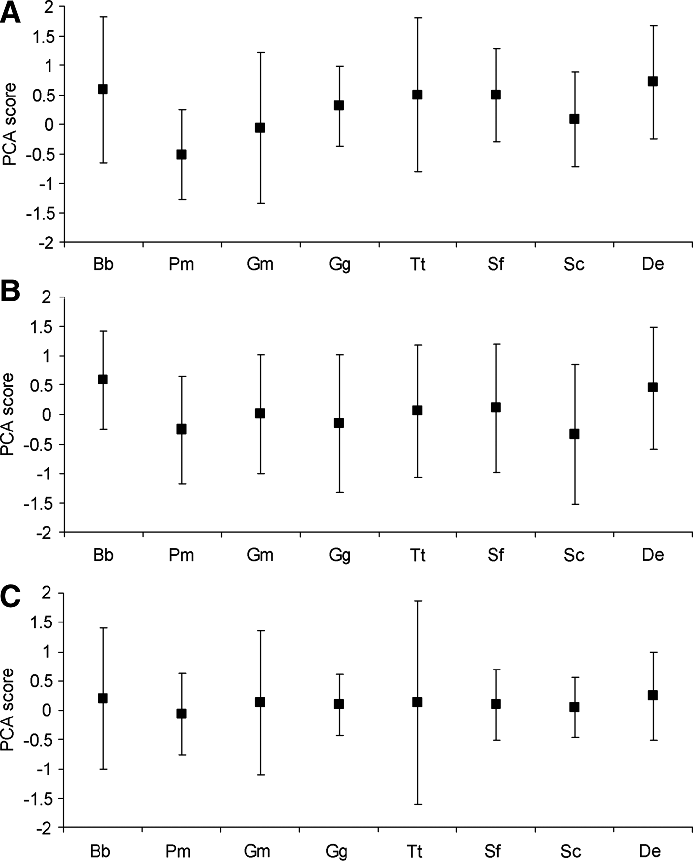
Variation along the first axis was explained predominantly by a negative relationship with water depth and SST (Table 2), with a high median PC score indicating an occurrence in shallower, cooler waters (Figure 3A). These data indicated that Physeter macrocephalus, Globicephala macrorhynchus and Stenella coeruleoalba occupied a deeper, warmer habitat niche than most other species. Delphinus sp. appeared to occupy the shallowest, coolest habitat (Figure 3A).

Fig. 3. Relative differences in the principal component analysis (PCA) score median and standard deviation between eight cetacean species for: (A) PC1, (B) PC2 and (C) PC3. Species abbreviations: Balaenoptera brydei (Bb), Physeter macrocephalus (Pm), Globicephala macrorhynchus (Gm), Grampus griseus (Gg), Tursiops truncatus (Tt), Stenella frontalis (Sf), Stenella coeruleoalba (Sco) and Delphinus sp. (De).
Sixteen species pairs differed significantly in PC score variance on the first axis, of which 12 remained significantly different after the Bonferroni correction was applied (Table 3). Globicephala macrorhynchus and Tursiops truncatus exhibited the highest number of significant differences (N = 5) with other species. Most species could be separated into two groupings that differed significantly from each other but did not exhibit intra-group differences: (1) Balaenoptera brydei, G. macrorhynchus and T. truncatus had relatively high levels of variation and may be considered to be generalists relative to the second group; and (2) Physeter macrocephalus, Grampus griseus, Stenella frontalis and S. coeruleoalba had relatively low levels of PC score variation and may be considered more specialized (Figure 3A). Delphinus sp. had an intermediate standard deviation and could not be clearly allocated to either group. This suggests that the group 1 species may, amongst other differences, inhabit a relatively wide range of water depths and SSTs, while the group 2 species occupy narrower depth and SST ranges (Figure 3A).
SECOND AXIS
There was significant variation in median PC scores of the eight cetacean species on the second axis (Kruskal–Wallis H = 39.82, df = 7, P < 0.001). Four pairwise comparisons that did not differ significantly on the first axis showed a significant difference in median PC score on the second axis (two remained significant following the Bonferroni correction) (Table 3). Balaenoptera brydei differed significantly in median PC score from Grampus griseus, Tursiops truncatus and Stenella frontalis, while T. truncatus versus Delphinus sp. also differed.
Variation along the second axis was mostly explained by a negative relationship with FS and SST (Table 2), with high median PC scores indicating an occurrence in waters of lower FS and SST (Figure 3B). The comparisons suggested that Balaenoptera brydei was recorded in waters of higher FS and/or warmer SST relative to Grampus griseus, Tursiops truncatus and Stenella frontalis (Figure 3B), and that Delphinus sp. was recorded in areas of higher FS and/or warmer SST relative to T. truncatus.
Three of the species pairs that did not differ significantly in PC score variance on the first axis were significantly different on the second axis (none remained significant following the Bonferroni correction) (Table 3). Physeter macrocephalus differed significantly from Grampus griseus and Stenella coeruleoalba suggesting that it was recorded in a narrower range of FS and SSTs relative to those species (Figure 3B). Balaenoptera brydei versus Tursiops truncatus was also significant, suggesting that B. brydei was recorded over a relatively narrow FS and SST range relative to T. truncatus (Figure 3B).
THIRD AXIS
There was significant variation in median PC scores of the eight cetacean species on the third axis (Kruskal–Wallis H = 21.93, df = 7, P < 0.005). Of the species pairs that did not differ significantly in median PC score or PC score variance on the first and second axes, only one species comparison was significant on the third axis: Stenella coeruleoalba and Delphinus sp. differed significantly in PC score variance. Variation along the third axis was explained predominantly by a strong negative relationship with slope (Table 2). Therefore, the data suggested that Delphinus sp. was recorded over a relatively wider range of seabed slopes than Stenella coeruleoalba (Figure 3C).
DISCUSSION
Redfern et al. (Reference Redfern, Ferguson, Becker, Hyrenbach, Good, Barlow, Kaschner, Baumgartner, Forney, Ballance, Fauchald, Halpin, Hamazaki, Pershing, Qian, Read, Reilly, Torres and Werner2006) noted that the purpose of a cetacean-habitat model determines the appropriate statistical tools that can be applied. This study examined the relative habitat preferences of cetaceans within a range of sampled habitats and compared cetacean niches in terms of the locations sampled, rather than attempting to describe absolute habitat preferences or predict cetacean occurrence in unsurveyed habitat. While the habitat preferences of some of the cetacean species considered in this study have been investigated in other geographical areas, only casual relationships with environmental variables (primarily water depth) have been previously noted in the eastern tropical Atlantic (Weir, Reference Weir2007; Picanço et al., Reference Picanço, Carvalho and Brito2009; de Boer, Reference de Boer2010). The present study used an extensive (both spatially and temporally) dataset and four EGVs to specifically examine cetacean habitat preferences and niche partitioning in the eastern tropical Atlantic, with implications for future management.
Habitat preferences
The classification tree (CT) analyses were limited to only four EGVs and did not evenly sample all available habitats. Therefore, the habitat preferences identified for the eight species can only be considered as relative to the sampled habitat, rather than absolute. Furthermore, as mentioned previously, there are caveats about the nature of the absence data. Nevertheless, the use of CTs provided a means of determining presence of each species in relation to the investigated EGVs, and identifying the most important EGV (of those examined) determining the occurrence of each species. While CTs are a relatively new method of investigating cetacean habitat preferences (Macleod & Zuur, 2005; Redfern et al., Reference Redfern, Ferguson, Becker, Hyrenbach, Good, Barlow, Kaschner, Baumgartner, Forney, Ballance, Fauchald, Halpin, Hamazaki, Pershing, Qian, Read, Reilly, Torres and Werner2006; MacLeod et al., Reference MacLeod, Weir, Pierpoint and Harland2007), tree-based models offer the advantage of being easy to interpret, since only EGVs that create homogeneous datasets and therefore explain some of the variation in species presence are retained in the model (Redfern et al., Reference Redfern, Ferguson, Becker, Hyrenbach, Good, Barlow, Kaschner, Baumgartner, Forney, Ballance, Fauchald, Halpin, Hamazaki, Pershing, Qian, Read, Reilly, Torres and Werner2006).
The CTs indicated that, of the EGVs considered, the presence of the majority of species (N = 7) within the study area was most influenced by SST (N = 4) or water depth (N = 3). Areas of cooler water were preferred by Balaenoptera brydei (<20.6°C) and Delphinus sp. (<22.1°C), while warmer water regions were preferred by Physeter macrocephalus (>23.6°C) and Globicephala macrorhynchus (>25.3°C). Within the study area, cooler water tends to occur in the region influenced by the Benguela Current upwelling in a band extending northwards along the coast from southern Angola, while warmer water occurs year-round in the oceanic environment. Consequently, the differences in SST preferences between these four species may partly reflect their occurrence in neritic versus oceanic habitat.
Frontal strength also appeared to be an important EGV determining the presence of Delphinus sp., which has been linked with areas of cool upwelling elsewhere (Au & Perryman, Reference Au and Perryman1985; Reilly, Reference Reilly1990; Ballance & Pitman, Reference Ballance and Pitman1998; Jefferson et al., Reference Jefferson, Fertl, Bolaños-Jiménez and Zerbini2009). A preference for cooler, productive water may at least partly explain the winter peak in occurrence of Delphinus sp. off northern Angola (Weir, Reference Weir2011), at a time when the Benguela Current extends furthest northwards within the study area (Hardman-Mountford et al., Reference Hardman-Mountford, Richardson, Agenbag, Hagen, Nykjaer, Shillington and Villacastin2003).
Water depth was the most important variable explaining presence for three cetacean species, and was the second most important variable for two further species. This EGV had been previously identified as a primary factor determining the distribution of species within the study area (Weir, Reference Weir2007, Reference Weir2011) and elsewhere (e.g. Davis et al., Reference Davis, Fargion, May, Leming, Baumgartner, Evans, Hansen and Mullin1998, Reference Davis, Ortega-Ortiz, Ribic, Evans, Biggs, Ressler, Cady, Leben, Mullin and Würsig2002; Baumgartner et al., Reference Baumgartner, Mullin, May and Leming2001; Waring et al., Reference Waring, Hamazaki, Sheehan, Wood and Baker2001; Cañadas et al., Reference Cañadas, Sagarminaga and García-Tiscar2002; Rossi-Santos et al., Reference Rossi-Santos, Wedekin and Sousa-Lima2006). The depth-related habitat preferences identified in the CTs were consistent with previous findings regarding neritic and oceanic cetacean communities in the study area (Weir, Reference Weir2007, Reference Weir2011). The deep-water preferences of Globicephala macrorhynchus and Physeter macrocephalus confirm their occurrence in the oceanic cetacean community and absence within neritic areas. Weir (Reference Weir2011) recorded highest sighting rates of G. macrorhynchus in upper slope waters, while the occurrence of P. macrocephalus in waters >1000 m depth has been well-documented throughout its known range (e.g. Rice, Reference Rice, Ridgway and Harrison1989; Davis et al., Reference Davis, Fargion, May, Leming, Baumgartner, Evans, Hansen and Mullin1998, Reference Davis, Ortega-Ortiz, Ribic, Evans, Biggs, Ressler, Cady, Leben, Mullin and Würsig2002; Baumgartner et al., Reference Baumgartner, Mullin, May and Leming2001; Waring et al., Reference Waring, Hamazaki, Sheehan, Wood and Baker2001).
Evidence for niche partitioning
The eight resident cetacean species exhibited overlap in their spatial and temporal distributions, and consequently in their occupied relative niches. This was not unexpected, since tropical oceanic odontocete species are known to: (1) usually occur within tropical areas on a year-round basis (i.e. without strong seasonal movements); (2) be wide-ranging; (3) aggregate in locations where prey is plentiful; and (4) sometimes form mixed-species schools (Au & Perryman, Reference Au and Perryman1985; Reilly, Reference Reilly1990; Bearzi, Reference Bearzi2005; Ballance et al., Reference Ballance, Pitman and Fiedler2006). Furthermore, the niche occupied by a species also has trophic components (Bearzi, Reference Bearzi2005). Consequently, ecologically-similar species that overlap in habitat may be segregated by factors such as prey type and size or foraging depth which were not analysed in the present study.
The high mobility of cetaceans can confuse interpretation of species–habitat relationships, since animals may be sighted while travelling over unsuitable habitat between patches of preferred habitat (Hamazaki, Reference Hamazaki2002; Ballance et al., Reference Ballance, Pitman and Fiedler2006). This is particularly true in tropical waters where prey may be unpredictable and patchily distributed (Weimerskirch et al., Reference Weimerskirch, Le Corre, Jaquemet and Marsac2005). Consequently, even in studies where strong significant relationships are found between cetacean species and EGVs, the EGVs may only partially explain variation in the occurrence of species within the cetacean community (Reilly & Fiedler, Reference Reilly and Fiedler1994; Ballance et al., Reference Ballance, Pitman and Fiedler2006).
Separate inshore and offshore populations or ecotypes of some species may exist within the study area and analysing such species as single categories with respect to their habitat niche may also obscure the findings. Compared with the other species, Balaenoptera brydei, Tursiops truncatus and Delphinus sp. occupied the widest and least specialized niches within the study area, incorporating a range of habitats extending from the coast to abyssal waters. However, there is evidence from other regions that separate inshore and offshore ecotypes of Tursiops dolphins (Hoelzel et al., Reference Hoelzel, Potter and Best1998) and of Balaenoptera brydei (Best, Reference Best2001) may occur. Similarly, the unresolved taxonomy of Delphinus dolphins in the region (Weir & Coles, Reference Weir and Coles2007) may also mask niche differences, since in the north-east Pacific D. delphis and long-beaked common dolphins (D. capensis) occupy different habitat (Heyning & Perrin, Reference Heyning and Perrin1994). Consequently, although B. brydei, T. truncatus and Delphinus sp. appeared to have rather wide ecological niches relative to the other species in the study area, this might not be the case if more than one ecotype, population or species occurs in the eastern tropical Atlantic.
Within the habitats sampled, the PC scores on the first axis were most strongly related to water depth and SST, as would have been expected from the CT results, and thus contributed most to the observed niche differences. Nineteen of the 28 pairwise comparisons exhibited significant differences in median first axis PC score (i.e. niche centre), while 16 pairs differed significantly in first axis PC score variance (i.e. niche width). Many studies have found relationships between depth, SST and cetacean occurrence, and most concluded that these relationships were the indirect result of environmental influences on the distribution of cetacean prey species (e.g. Cañadas et al., Reference Cañadas, Sagarminaga and García-Tiscar2002; Davis et al., Reference Davis, Ortega-Ortiz, Ribic, Evans, Biggs, Ressler, Cady, Leben, Mullin and Würsig2002; Doksæter et al., Reference Doksæter, Olsen, Nøttestad and Fernö2008). The narrow and distinct (deeper and warmer water) niche occupied by Physeter macrocephalus in the eastern tropical Atlantic may reflect the higher trophic level and larger prey sizes of this species relative to others (Pauly et al., Reference Pauly, Trites, Capuli and Christensen1998; MacLeod et al., Reference MacLeod, Santos, López and Pierce2006). Like P. macrocephalus, Globicephala macrorhynchus and Grampus griseus are primarily cephalopod-eaters (Clarke, Reference Clarke1996; Pauly et al., Reference Pauly, Trites, Capuli and Christensen1998) and occupy predominantly oceanic waters (e.g. Davis et al., Reference Davis, Fargion, May, Leming, Baumgartner, Evans, Hansen and Mullin1998, Reference Davis, Ortega-Ortiz, Ribic, Evans, Biggs, Ressler, Cady, Leben, Mullin and Würsig2002; Cañadas et al., Reference Cañadas, Sagarminaga and García-Tiscar2002; Praca & Gannier, Reference Praca and Gannier2008). The increase in median water depth of occupied grid cells from G. griseus to P. macrocephalus (Table 4) coincides with increased body size, foraging dive duration, typical foraging depth, trophic level and a change in diet composition from small to large squid species. Consequently, in addition to relative differences in the habitat occupied, these three cephalopod-eating species may avoid competition by targeting slightly different prey sizes (e.g. MacLeod et al., Reference MacLeod, Santos, López and Pierce2006) or by foraging at different levels in the water column (e.g. MacLeod et al., Reference MacLeod, Hauser and Peckham2004).
Table 4. Median and standard deviation (SD) (a measure of variance) of the ecogeographical variables in the grid cells for eight cetacean species.

SST, sea surface temperature; FS, frontal strength; for species names in full see Table 1.
The two Stenella species and Delphinus dolphins are ecologically similar species with comparable morphology, diet, diving capabilities and group sizes, and these species may be expected to compete when occurring in the same habitat. The combined results of the CT analysis and PCA suggested some niche partitioning amongst these species, with S. coeruleoalba occurring in relatively deeper and warmer waters and of steeper seabed slope than Delphinus sp., and S. frontalis occupying intermediate regions. In an investigation of the habitat preferences of the Stenella genus in the south-west Atlantic, Moreno et al. (Reference Moreno, Zerbini, Danilewicz, de Oliveira Santos, Simões-Lopes, Lailson-Brito and Azevedo2005) found that S. frontalis sightings occurred in median SSTs of 22.6°C. Both that study, and the present study, indicated that within subtropical/tropical Atlantic waters Stenella frontalis may occupy cooler waters relative to other Stenella species.
Niche partitioning has been suggested between sympatric Stenella and Delphinus dolphins in the eastern tropical Pacific, where S. longirostris and S. attenuata preferred warm waters with sharp thermoclines while D. delphis and S. coeruleoalba preferred cooler, mixed waters with greater upwelling (Au & Perryman, Reference Au and Perryman1985). However, a later study in the same area suggested that S. coeruleoalba was poorly described by habitat variables and that its distribution overlapped with the other species (Reilly, Reference Reilly1990; Reilly & Fiedler, Reference Reilly and Fiedler1994). In the Gulf of Mexico, the habitat of five Stenella species overlapped but could partly be partitioned by depth, with S. frontalis occurring predominantly on the shelf, S. longirostris over the slope and S. attenuata, S. coeruleoalba and the Clymene dolphin (Stenella clymene) inhabiting the deepest areas (Davis et al., Reference Davis, Ortega-Ortiz, Ribic, Evans, Biggs, Ressler, Cady, Leben, Mullin and Würsig2002; Maze-Foley & Mullin, Reference Maze-Foley and Mullin2006).
Not all studies have found clear evidence of niche partitioning between sympatric Stenella and Delphinus species. For example, Gross et al. (Reference Gross, Kiszka, Van Canneyt, Richard and Ridoux2009) found no obvious partitioning between S. attenuata and S. longirostris in either habitat or diet in the south-west Indian Ocean, while Pusineri et al. (Reference Pusineri, Chancollon, Ringelstein and Ridoux2008) found considerable overlap in size, diversity and type of prey species taken by D. delphis and S. coeruleoalba in the Bay of Biscay (both were assumed to forage at similar depths and nocturnally). Clua & Grosvalet (Reference Clua and Grosvalet2001) recorded D. delphis and S. frontalis associating and foraging together in the Azores. Presumably in such instances prey availability was not a limiting resource, and/or mixed-species associations may have conferred some additional benefit such as increased predator avoidance (i.e. for large sharks and killer whales Orcinus orca) or improved foraging efficiency.
Only two species pairs did not differ significantly from each other on any of the three PC axes considered in these analyses (Table 3). Balaenoptera brydei and Delphinus sp. inhabited a comparable range of habitats in terms of water depth and SST. Similarly, Grampus griseus and Stenella frontalis exhibited very similar niche centres and widths, both showing a preference for warm waters along the slope. Neither of these species pairs is likely to experience particularly high levels of interspecific competition. The offshore population of B. brydei feeds on a variety of fish and euphausiid species in the study area (Best, Reference Best2001), while Delphinus sp. and S. frontalis are likely to prey opportunistically on various shoaling fish and cephalopod species (Pauly et al., Reference Pauly, Trites, Capuli and Christensen1998). Grampus griseus primarily feeds upon small and large cephalopods (Pauly et al., Reference Pauly, Trites, Capuli and Christensen1998). Consequently, these particular species pairs may be able to coexist in the same habitats by exhibiting foraging differences.
Use of a novel technique to examine cetacean niches
The technique used to examine relative cetacean niches in this paper was developed in response to: (1) the use of data collected from non-dedicated platforms where the distribution of survey effort could not be controlled; and (2) the lack of available absence data to permit more traditional methods of niche analysis. Datasets gathered from non-dedicated platforms represent a potentially large and increasingly common source of cetacean data worldwide, and it is important to determine the potential for using them beyond simple descriptions of cetacean presence and without imposing too many assumptions. While the data presented here were not collected specifically to analyse cetacean–habitat relationships, the technique was able to identify statistically significant differences between some pairs of species in their median PC score and PC score variance. This technique also provided several advantages compared to some more established methods of analysing cetacean–habitat relationships: (1) the use of a PCA which summarizes the EGVs into several uncorrelated axes accounts for potential interactions between the EGVs, rather than considering them as individual variables as many traditional analyses do (potentially causing bias; Redfern et al., Reference Redfern, Ferguson, Becker, Hyrenbach, Good, Barlow, Kaschner, Baumgartner, Forney, Ballance, Fauchald, Halpin, Hamazaki, Pershing, Qian, Read, Reilly, Torres and Werner2006); (2) analysis of the PC scores allowed for specific testing of the differences in the relative niche centres and niche widths occupied by different species, an aspect of habitat comparison that is overlooked by many studies; and (3) the method provided an advance on studies that simply qualitatively compare the mean values for individual habitat variables without using any statistical verification.
The PCA method introduced in this study is based on the same general approach and theoretical basis as presence-only distribution models that have previously been applied to investigating cetacean distribution relative to environmental variables (e.g. MacLeod et al. Reference MacLeod, Weir, Pierpoint and Harland2007), such as the PCA-based model of Robertson et al. (Reference Robertson, Caithness and Villet2001) and Ecological-Niche Factor Analysis (ENFA) (Hirzel et al., Reference Hirzel, Hausser, Chessel and Perrin2002). However, rather than relying on presence data of a single species, the PCA method used here incorporated data on multiple species into a single analysis. This helped to eliminate issues associated with not knowing whether the absence of a species within a particular habitat was the result of the species not using that habitat, or the habitat not being surveyed. Therefore, including data from other species as data absence points provided a greater certainty that the habitat preferences identified for each species were real rather than an artefact of the distribution of survey effort in relation to the habitat variables examined (as may potentially be the case with presence-only modelling approaches such as ENFA).
The findings of the study are subject to several caveats arising from both the data source and the analysis technique: (1) the grid cells had a deep water bias since most of the survey work occurred in oceanic waters (Weir, Reference Weir2011); (2) the temporal analysis scale was limited by the availability of the environmental EGVs which had to be analysed as monthly composites because of insufficient satellite coverage (due to cloud) at higher resolution; (3) the number of EGVs analysed during the study was limited to four, while other EGVs may also be important in determining habitat niche; and (4) there is a potential impact on the observed species' niches if interspecific variation in response to airgun sound occurs.
While the first of these points is a potential source of heterogeneity relative to the EGVs, the data were analysed in a manner that investigated the evidence for cetacean niche partitioning within the sampled habitat (i.e. at positive sighting locations) rather than attempting to identify niches across all habitats. Consequently, the question being investigated is whether cetacean species have different niches within the sampled range, not whether they differ in niche across the entire available habitat within the study area.
Monthly composites should provide information on moderate-scale relationships between cetaceans and their habitat, and represent the typical ranges at which associations between EGVs and marine predators have been observed in other studies (Redfern et al., Reference Redfern, Ferguson, Becker, Hyrenbach, Good, Barlow, Kaschner, Baumgartner, Forney, Ballance, Fauchald, Halpin, Hamazaki, Pershing, Qian, Read, Reilly, Torres and Werner2006). However, they may not always be sufficient to identify fine-scale niche partitioning between similar species within an area. A large number of other EGVs have been implicated in cetacean habitat studies and, within the study area, turbidity and salinity (particularly due to the outflow of the Congo River), depth of the thermocline, chlorophyll-α concentration and prey distribution may also be important factors governing niche. While these could not be included in the current analyses, they should be examined during future work.
Some of the data analysed in this study were collected from geophysical survey vessels, and the potential for interspecific variation in response to airgun sound is clearly a factor when considering the proportions of species recorded (Weir, Reference Weir2007, Reference Weir2008). However, as long as each species responded consistently to airgun sound across the full range of available habitats (i.e. their response did not vary according to EGV values), this should not have influenced the outcomes of the study.
Implications for conservation and management
The ecological niche concept is one of several important considerations when identifying which species should be priorities for conservation, since, within their overall range, specialized species that occupy the smallest niches may be most vulnerable to displacement from anthropogenic impacts. Furthermore, knowledge of the factors governing the spatio-temporal occurrence of a species is crucial in interpreting abundance estimates (Smith et al., Reference Smith, Dustan, Au, Baker and Dunlap1986; Reilly & Fiedler, Reference Reilly and Fiedler1994), identifying critical habitat (Gregr & Trites, Reference Gregr and Trites2001; Bräger et al., Reference Bräger, Harraway and Manly2003), designating protected areas (Hooker et al., Reference Hooker, Whitehead and Gowns1999; Cañadas et al., Reference Cañadas, Sagarminaga and García-Tiscar2002; Hamazaki, Reference Hamazaki2002), identifying areas where core cetacean habitat and anthropogenic activities overlap (Baumgartner, Reference Baumgartner1997; Praca & Gannier, Reference Praca and Gannier2008), and predicting the likely impacts on species from climate change (Azzellino et al., Reference Azzellino, Gaspari, Airoldi and Lanfredi2008b; MacLeod et al., Reference MacLeod, Weir, Santos and Dunn2008).
Within the study area, SST and water depth were found to be the most important EGVs (of those considered) influencing cetacean occurrence, with most species occurring in warmer, oceanic portions of the study area. Furthermore, the eight species considered here are year-round residents within the study area (Weir, Reference Weir2007, Reference Weir2011), and the region is considered to represent core parts of their geographical range (rather than edge habitat). Consequently, further investigation of cetacean occurrence in warm areas seaward of the shelf edge may represent an appropriate starting point for maintaining cetacean biodiversity in the region.
ACKNOWLEDGEMENTS
The sightings analysed in this paper were recorded during fieldwork sponsored by (chronologically) GX Technology, BP Exploration (Angola) Ltd and their partners in Blocks 18 and 31, Esso Exploration Angola (Block 15) Ltd and their partners in Block 15, Total E&P Angola and their partners in Blocks 17 and 32, Total E&P Congo, Total E&P Gabon and Ophir Energy. Thanks to all of the observers, particularly Ian Austin, Nathan Gricks, Chris Pierpoint, Richard Shucksmith, Sue Travers, Michael Unwin, Frank Vargas and Richard Woodcock, for collecting the data used (in addition to that of C.W.) in this paper, and to the crews of the ‘Discoverer', ‘Geco Triton’, ‘Sea Trident', ‘Ramform Viking', ‘Remus', ‘Ramform Vanguard', ‘CGG Geo Challenger', ‘CGG Venturer', ‘Western Pride' and ‘Ramform Challenger' for their hospitality. Peter Miller, Rory Hutson, Ben Taylor and Peter Walker at Plymouth Marine Laboratory provided the SST, chlorophyll-α and frontal satellite derived maps (application to NEODAAS, NERC) and answered various related queries. Thanks to Ruth Fernández-García for assistance with the classification tree analysis.