


INTRODUCTION
The Mystacocarida are a small distinct group of interstitial crustaceans of subclass Maxillopoda, which includes the harpacticoid copepods, the only other group of interstitial crustaceans with which mystacocarids could be confused. The first mystacocarid species Derocheilocaris typicus was described by Pennak & Zinn (Reference Pennak and Zinn1943) from the interstitial fauna of sand beaches on the north-eastern coast of the North America. Worldwide 12 species have been described, divided between two genera, Derocheilocaris and Ctenocheilocaris (Hessler, Reference Hessler, Higgins and Thiel1988). In Chile, Derocheilocaris galvarini was described by Dahl (Reference Dahl1952) using material collected during the Lund University expedition to Chile (Brattström & Dahl, Reference Brattström and Dahl1951). The type location was coarse sand from a depth of 25 m at an anchorage near Punta Weather on the north west side of Isla Guafo (43.55°S 74.82°W). The species was named in honour of the Chilean Naval ship ‘Galvarino’. The only other paper that discusses Chilean Mystacocarida is by Noodt (Reference Noodt1961), in which he describes D. galvarini from semi-fine intertidal sands at Las Cruces, on the Litoral Central coast. In Reference Renaud-Mornant1976 Renaud-Mornant assigned D. galvarini to the genus Ctenocheilocaris (Figure 1). This paper outlines the current state of knowledge concerning the abundance, distribution and typical habitat of C. galvarini. The data presented here were collected as part of a larger study of the macroecology of meiofauna, particularly nematodes, along the coast of Chile.

Fig. 1. Adult Ctenocheilocaris galvarini from Ritoque (32.82961°S 71.52914°W) Valparaiso region. Scale bar = 250 μm.
MATERIALS AND METHODS
Quantitative and qualitative sampling was conducted at 66 sites, typically three sites per degree of latitude, along the exposed coast of Chile, from 18°S to 42°S, between March 2008 and November 2010 (see Figure 2 for a map of all the sites sampled). Five replicate quantitative samples of 50 cm3 were taken using a plastic syringe modified to form a piston corer (Chandler & Fleeger, Reference Chandler and Fleeger1983). The samples were taken randomly in the zone of retention of each beach, this being the zone of the beach that typically supports the highest abundance of meiofauna (McLachlan & Brown, Reference Mclachlan and Brown2006). Each sample was placed in a 110 ml plastic jar with approximately 50 ml of 5% formalin. The formalin solution was made up on site using 45 μm filtered seawater. On exposed beaches qualitative samples were taken from the following zones, dry (high shore), retention, resurgence and from the depth of the water-table; samples were also taken from any other apparent micro-habitat on the beach, temporary lagoons, streams that crossed the beach, beneath cast algae, for example. All samples were fixed with 5% formalin prepared as above. All samples were transported back to the laboratory for processing and analysis.
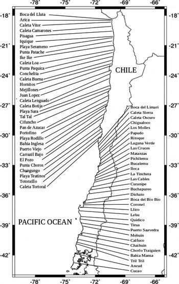
Fig. 2. Map of the study sites along the coast of Chile. More details on each site can be found at: http://meiochile.matthewlee.org/?page_id=480/.
The meiofauna from each quantitative sample was extracted using a two stage methodology. The fauna was removed from the substrate by the decantation method (Pfannkuche & Thiel, Reference Pfannkuche, Thiel, Higgins and Thiel1988), using 45 μm filtered fresh water. The extraction procedure was repeated five times. The material captured on the 45 μm sieve by the decantation method was then further processed using the Ludox flotation method (Burgess, Reference Burgess2001). This removes any remaining sediment from the sample. The samples were washed into 250 ml beakers with Ludox (a colloidal silica solution with a density of 1.14). The samples were then left for 1 h for the density separation to take place, after which the Ludox was poured slowly through a 45 μm sieve with care being taken not to re-suspend the sediment at the bottom of the beaker. The meiofauna in the qualitative samples was extracted using the same basic methodology, but extraction with Ludox was not used where no sediment remained in the sample after decantation.
The fauna extracted from the quantitative samples was then washed into embryo dishes with a glycerol solution (5% glycerol, 20% ethanol, 75% distilled water) and placed in a warm desiccator for a period of between 24 and 48 h. Once the water and alcohol had evaporated leaving the fauna in glycerol the samples were mounted on a large glass microscope slides (75 × 38 mm) within a wax ring. Where the fauna was present in very high densities or where there was a significant amount of organic material in a sample, the sample was divided between two or more slides to facilitate analysis. The analysis of each slide was conducted using an Olympus BX 51 compound microscope equipped with DIC illumination and a drawing tube. The entire slide was scanned at ×100, and the abundance of Mystacocarida was recorded. Fauna from the qualitative samples was washed into a Petri dish and examined under a stereo microscope. The presence or absence of Mystacocarida, as with all the other meiofaunal groups, was recorded.
The sediments from which the fauna was extracted were analysed using settling velocities in an Emery tube (Emery, Reference Emery1938). The majority of the general environmental data were obtained from Aquamaps.org (Kaschner et al., Reference Kaschner, Ready, Agbayani, Rius, Kesner-Reyes, Eastwood, South, Kullander, Rees, Close, Watson, Pauly and Froese2008). In addition to latitude (°S), the following environmental data were used: fractal dimension of the coast line (D), mean annual sea surface temperature (SST) in °C, and mean annual primary productivity (PP) in mgC m−2 d−1. The fractal dimension of the coastline (D), a measure of coastline complexity, was calculated for each degree of latitude, between 18°S and 42°S, using images of the coastline obtained from the US National Oceanic and Atmospheric Administration online coastline extractor tool (http://www.ngdc.noaa.gov/mgg_coastline/index.jsp), these images were then processed using Gwyddion image processing software (v.2.13), using linear interpolation and the cube counting method to yield the fractal dimension (D). To check whether there was any bias introduced by the month of the year during which sampling took place, the variable ‘Sampling Time’ (S.Time) with a scale from 1 to 12, was created; austral summer months had low values, winter months high values. Standard Pearson's correlations and linear regressions were made using R (R Core Team, 2013).
RESULTS
Ctenocheilocaris galvarini was found at 11 of the 66 sites sampled along the exposed coast of Chile between 18°S and 42°S. Specimens were found in quantitative samples from Matanzas, Bucalemu, Iloca, Llico, Calfuco and Chaihuin, and in qualitative samples from Tirua, Calfuco, Chaihuin, Tril Tril and Cucao (Table 1). Ctenocheilocaris galvarini has also been observed in samples from Las Cruces and Ritoque (M. Lee, personal observation), but not during the current sampling campaign.
Table 1. Details of the samples and sites where Ctenocheilocaris galvarini was found. Latitudes and longitudes are given in decimal values. Average abundances (ind 50 cm−3) are given for the quantitative samples.

Ctenocheilocaris galvarini abundance in the quantitative samples varied from a single individual (Matanzas and Iloca) to 56 individuals in one sample from Llico. Average abundances varied from 0.2 to 20.4 ind 50 cm−3. In the current sampling campaign C. galvarini was not observed north of 33°S, and the most northerly record was from Ritoque (32°S) (M. Lee, personal observation). All the sites where C. galvarini has been observed are exposed beaches with intermediate morphology (Short & Wright, Reference Short, Wright, McLachlan and Erasmus1983) with fine well-sorted sands with a skew towards finer sizes (averages: Md = 2.01, QDI = 0.44, SkI = −0.63, see Table 2 for the data for each site and zone). C. galvarini was present in 16.7% of the sites sampled. Of the 66 sites sampled 28 were of intermediate morphology (57.6%). Thus, Ctenocheilocaris galvarini was present in 39.3% of intermediate beaches along the coast of Chile, and present in 73.3% of intermediate beaches south of and including Ritoque (32°S).
Table 2. Sediment parameters for each of the sites where Ctenocheilocaris galvarini was found. Md, graphic mean; Wentworth, Wentworth scale; QDI, inclusive graphic quartile deviation; SkI, inclusive graphic skewness.

There were no significant correlations between log transformed C. galvarini abundance and sampling time, latitude, mean annual sea surface temperature, coastal complexity or mean annual primary productivity. There was an apparent increase in C. galvarini abundance with increasing latitude, but this trend was not statistically significant.
DISCUSSION
Previous information on C. galvarini in Chile was extremely scarce, consisting of only two papers (Dahl, Reference Dahl1952; Noodt, Reference Noodt1961). The information presented in the current paper allows a number of new conclusions to be drawn concerning both the geographic distribution and habitat of C. galvarini.
The original type specimen was collected in sub-tidal waters off Isla Guafo (43.55°S 74.82°W) in the Los Lagos region, and this is the most southerly site where this species has been recorded. The most northerly site where it has been observed is Ritoque (32.82961°S 71.52914°W) in the Valparaiso region, and the most southerly Isla Guafo (43.55°S 74.82°W) (Dahl, Reference Dahl1952). Given that 42 sites were sampled north of Ritoque all the way up to the border with Peru, and not a single specimen of C. galvarini was recorded, despite the presence of appropriate habitat (see below), it is valid to assume that the presence of C. galvarini north of Ritoque is very infrequent, if it occurs at all. Thus, the current known geographic distribution of C. galvarini is between 32°S and 44°S.
The samples collected also allow the habitat of C. galvarini to be described with more certainty. The original type habitat was coarse sand at a depth of 25 m. The current sampling regime was confined to intertidal habitats, so for the moment it is unknown whether C. galvarini is common in the sub-tidal or only occasional; Dahl (Reference Dahl1952) refers to ‘numerous specimens’ but does not give an abundance figure. However, in none of the samples from the current sampling regime was C. galvarini found associated with coarse sediment. Noodt (Reference Noodt1961) describes C. gavarini from intertidal ‘semi-fine’ grained sediments, from a sediment depth of 20 cm and an abundance of one adult and two juveniles; he does not state the sample volume. Noodt's (Reference Noodt1961) sample was from Las Cruces. Although he does not specify which beach or give precise coordinates, based on the site description it is likely that he is referring to the large intermediate beach Playa Grande (33.52°S 71.61°W), which extends from the south side of Las Cruces down to Cartagena, where C. galvarini has been observed more recently (M. Lee, personal observation). The abundance data presented in the current paper are all from quantitative samples collected in the retention zone between 0 and 10 cm depth. Ctenocheilocaris galvarini was also recorded in qualitative samples from the zones of retention (Tirua), resurgence (Tirua, Chaihuin) and sub-littoral fringe (Tirua), as well as from sediment in a temporary back-shore lagoon (Tirua) and in samples from the depth of the water-table (Calfuco and Cucao, depth approximately 30 cm at both sites). All samples, both quantitative and qualitative, that contained C. galvarini came from beaches with intermediate morphology (Short & Wright, Reference Short, Wright, McLachlan and Erasmus1983) and fine well-sorted sand (Wentworth scale, equates to a mean sediment grain size of 250 μm or +2 on the φ scale). Based on these observations, the typical intertidal habitat of C. galvarini can be described as intermediate beaches, the majority of which have fine sand. The depth in the sediment is probably below the surface down to the interface with the water table, though more sampling is necessary to confirm this. It may be that the low abundances observed in the majority of the quantitative samples was due to C. galvarini being present deeper in the sediment than the sampling depth of the corer. It is notable that the highest abundances were found at Llico, where the water table was shallow, at around 20 cm deep, making it more likely that C. galvarini would be sampled by the quantitative methodology. Noodt's (Reference Noodt1961) conclusion was that C. galvarini was distributed sub-tidally and only occasionally found in the intertidal. The currently available information, however, does not confirm this, but indicates that C. galvarini is an intertidal species. Further sampling will be required to determine the sub-tidal abundances and habitat of this species.
Mystacocarida are, like the majority of the meiofauna, direct benthic recruiters, lacking a pelagic larval phase. Given the patchy distribution of C. gavarini and their direct benthic recruitment, an interesting question for future research is: how do they disperse? The assumption is that transport of individuals between beaches is either the result of random events such as rafting or long-term dispersion through interconnected, sub-tidal patches of suitable habitat. Given also the extreme morphological conservatism (Hessler, Reference Hessler, Higgins and Thiel1988) of the Mystacocarida these questions should ideally be examined with the aid of molecular techniques.
In summary, C. galvarini is found primarily in southern Chile, south of 32°, in the intertidal of intermediate beaches with fine sand, most likely distributed between the level of the water-table and the surface, but avoiding dry sand.
ACKNOWLEDGEMENTS
Exequiel Sanhueza assisted with fieldwork during the first year of the project. Thanks go to Dr Martin Thiel for his constructive criticism of an earlier version of this manuscript.
FINANCIAL SUPPORT
Funding for this research was provided by Fondecyt grant 1080033 (to M.R.L.).


