


Introduction
Natural mortality (M) is a fundamental parameter to understand the dynamics of harvested populations (Kenchington, Reference Kenchington2014) and to develop conservation and management procedures. The magnitude of M is directly related to the productivity of the population, environmental forces, exploitation rates, management variables (e.g. maximum sustainable yield) and biological reference points (Brodziak et al., Reference Brodziak, Ianelli, Lorenzen and Methot2011). In stock assessments, M is important for its proportion of total mortality which is divided into natural causes vs exploitation (fishing mortality), so it is crucial to understand the effect of exploitation and its impact on sustainable catches (Hewitt, Reference Hewitt2008; Gislason et al., Reference Gislason, Niels, Rice and Pope2010). Unfortunately, natural mortality is also one of the most difficult quantities to estimate (Brodziak et al., Reference Brodziak, Ianelli, Lorenzen and Methot2011; Kenchington, Reference Kenchington2014) and normally the M estimate for assessment analysis comes from external sources and needs to be specified beforehand.
From a biological standpoint, factors that explain M can be divided into intrinsic and extrinsic forces (Brodziak et al., Reference Brodziak, Ianelli, Lorenzen and Methot2011). The former is related to the correlation reported from studies of lifespan (maximum age), body size and senescence, as well as links between metabolic rate and body mass adjusted for habitat temperature (Brown et al., Reference Brown, Gillooly, Allen, Savage and West2004). Fish and aquatic invertebrate mortality arise from a combination of size-dependent and life history stage/age-dependent processes (Lorenzen, Reference Lorenzen1996; Andersen et al., Reference Andersen, Farnsworth, Pedersen, Gislason and Beyer2009; Gislason et al., Reference Gislason, Niels, Rice and Pope2010). These processes include reproduction, senescence and starvation, and vary with size and age, resulting in natural mortality patterns in ‘L' or ‘U’ shape (Beverton & Holt, Reference Beverton, Holt, Wolstenholme and O'Connor1959; Lorenzen, Reference Lorenzen2011). For instance, for some species M will be larger in egg and larval stages than in juvenile ones, but M could also be higher for juveniles and adults. M could also stabilize in adults due to the higher metabolic costs of reproduction (intrinsic mortality), reducing M as individuals’ body size increases and they become less vulnerable to predation (Lorenzen, Reference Lorenzen1996; Beverton et al., Reference Beverton, Hylen, Østvedt, Alvsvaag and Iles2004). In most decapod crustaceans, mortality is high in the early life periods and rather low for adults; however, sensitive life phases like hatching, transition from lecithotrophy to active feeding or transition from planktonic to benthic life showed high mortality (Vogt, Reference Vogt2011). Crustaceans undergo moulting and, in many species, individuals are vulnerable to an enlarged suite of predators during this process. For instance, crabs are most vulnerable to predation before, during and after moulting (Ryer et al., Reference Ryer, van Montfrans and Moody1997). In addition, several studies have shown that natural mortality in harvested crustacean species varies with age, sex and time (Fu & Quinn, Reference Fu and Quinn2000; Xiao & McShane, Reference Xiao and McShane2000). Crustacean decapods apparently do not suffer from reproductive senescence, possibly due to a double function of the moult inhibiting hormones as is observed in blue crab Callinectes sapidus (Zmora et al., Reference Zmora, Trant, Zohar and Chung2009).
Extrinsic factors that determine M (i.e. external sources of mortality) do not allow individuals to reach their life expectancy. Examples include disease, predation, food availability, or other causes of death – except fishing exploitation. For instance, species at a high trophic level may show more consistent patterns with single-species models, where fishing mortality dominates over M, than with those from an intermediate trophic level that depend more on trophic web processes, with predation mortality taking prevalence over fishing mortality (Gaichas et al., Reference Gaichas, Aydin and Francis2010). Episodic mortality, such as epidemics or red tides, could also be relevant (Brodziak et al., Reference Brodziak, Ianelli, Lorenzen and Methot2011). For instance, parasitic dinoflagellates, e.g. Hematodinium, are well known as a significant disease agent of commercially important crustaceans such as blue crabs and Norway lobster Nephrops norvegicus and cause economic losses to fisheries by increasing mortality (Hamilton et al., Reference Hamilton, Shaw and Morrit2009; Huchin-Mian et al., Reference Huchin-Mian, Small and Shields2017). In Chile, infestation by Pseudione humboldtensis in red squat lobster Pleuroncodes monodon and yellow squat lobster Cervimunida johni has been identified as affecting reproduction, inhibiting growth and producing nutritional deficiencies (Gonzalez & Acuña, Reference Gonzalez and Acuña2004). These authors suggest that the parasitic infestation along with a depleted stock can create synergies that affect the sustainability of these fisheries. Compensation mortality plays an important role when resources are scarce, especially during juvenile stages (Brodziak et al., Reference Brodziak, Ianelli, Lorenzen and Methot2011).
Although M is an important parameter, it is hard to estimate (Vetter, Reference Vetter1988; Quiroz et al., Reference Quiroz, Wiff and Caneco2010; Brodziak et al., Reference Brodziak, Ianelli, Lorenzen and Methot2011; Kenchington, Reference Kenchington2014). The natural mortality rate can be estimated directly through methods such as catch curves, mark-recapture or telemetry. But in addition to difficult implementation, these methods also need an extensive amount of data and are expensive (Quiroz et al., Reference Quiroz, Wiff and Caneco2010; Kenchington, Reference Kenchington2014). An alternative approach is to use indirect methods that are based on life history correlations (Kenchington, Reference Kenchington2014; Hoenig et al., Reference Hoenig, Then, Babcock, Hall, Hewitt and Hesp2016). These methods predict M from the trade off between natural mortality and life history traits, e.g. the somatic growth rate (k) and maximum age (Beverton & Holt, Reference Beverton, Holt, Wolstenholme and O'Connor1959) and further allow providing point length/age-based estimates of M (Peterson & Wroblewski, Reference Peterson and Wroblewski1984; Charnov & Berrigan, Reference Charnov and Berrigan1991; Lorenzen, Reference Lorenzen1996).
Direct estimates of M in crustaceans are scarce due to the difficulties of measuring (i.e. quantifying) and monitoring discontinuity of their somatic growth (moults). This type of growth removes the hard parts that could work for age determination and in the case of the mark-recapture, marks can get lost due to the moulting process, which also complicates direct studies to estimate M (Hewitt, Reference Hewitt2008). Direct estimates of M in crustaceans are both limited and variable (Vogt, Reference Vogt2011). For instance, M values for large crustaceans such as rock lobster Jasus edwardsii have been estimated at 0.12 (year−1) (Frusher & Hoenig, Reference Frusher and Hoenig2001) and from 2.7 to 6.8 (year −1) in green tiger prawn (Penaeus semisulcatus) (Hussain et al., Reference Hussain, Bishop and Xu1996). Thus, the inconvenience of M direct determination in crustaceans requires the estimation of M to be based on indirect methods usually developed for fish population stock assessment.
In Chile, yellow and red squat lobster are two of the most important crustaceans harvested in terms of landings and economic significance. These demersal species inhabit the South-eastern Pacific (Figure 1). Off the Chilean coast they are distributed between 24°30′S and 37°00′S (C. johni) and between 18°25′S and 37°00′S (P. monodon). The fisheries for these species generally occur from 27°30′S to 37°S (C. johni) and from 26°30′S to 37°S (P. monodon). A discontinuity in the distribution of P. monodon is found between 30°S and 32°S (Roa & Tapia, Reference Roa and Tapia1998; Wehrtmann & Acuña, Reference Wehrtmann, Acuña, Poore, Ahyong and Taylor2011). Their distribution is also characterized by a narrow band along the continental shelf and upper part of the continental slope at depths of 100 to 500 m.

Fig. 1. Distribution of Cervimunida johni (yellow squat lobster (A) and Pleuroncodes monodon (red squat lobster) (B) off the Chilean coast (23°–38°S). Note the discontinuity in the distribution of P. monodon between 30°S and 32°S.
The commercial squat lobster fisheries in Chile started in the 1950s associated to the hake (Merluccius gayi) fishery (Arana et al., Reference Arana, Melo, Noziglia, Sepúlveda, Silva, Yany and Yáñez1975; Wehrtmann & Acuña, Reference Wehrtmann, Acuña, Poore, Ahyong and Taylor2011). Industrial and small-scale bottom trawlers achieved record landings of around 10,000 tons (1997) and 62,000 tons (1976) for yellow and red squat lobster, respectively. Nowadays, landings of both species are below 9000 tons and for management purposes the squat lobster fisheries are divided into two fishery units, whose limit is set at 32°10′S. In addition, management of both squat lobsters is based on total allowed catch (TAC) and seasonal closures of the fishery units (Bucarey, Reference Bucarey2015a, Reference Bucarey2015b). The TAC system requires annual estimates of abundance based on an integrated assessment model, where M is a key parameter determined beforehand. Current estimates of M for the yellow and red squat lobster are based on the indirect methods of Alverson & Carney (Reference Alverson and Carney1975), Rikhter & Efanov (Reference Rikhter and Efanov1976), Pauly (Reference Pauly1980), Hoenig (Reference Hoenig1983), Alagaraja (Reference Alagaraja1984) and Jensen (Reference Jensen1996) characterized by point estimate averages across ages/lengths (Bucarey, Reference Bucarey2015a, Reference Bucarey2015b). However, the applicability of these methods in the context of crustacean species has not been reviewed nor has uncertainty been included. The aim of this paper is to estimate M in both squat lobster species accounting for (i) the theoretical basis of the indirect method applied, and (ii) the uncertainty of M estimates.
Methods
Indirect methods to estimate M crustaceans
The first step was selecting the indirect methods with potential for crustaceans, that is, methods based on general principles, e.g. life history (Beverton & Holt, Reference Beverton, Holt, Wolstenholme and O'Connor1959), that are shared across harvested populations and can be applied to marine invertebrates. We based our revision on Brodziak et al. (Reference Brodziak, Ianelli, Lorenzen and Methot2011) and Kenchington (Reference Kenchington2014), the first categorized the methods in groups, or tiers, where Tier 1 accounts for the traditionally accepted (‘rule-of-thumb’) values such as M = 0.2 (year−1), and those estimated from meta-analysis or based on life history theory (Beverton & Holt, Reference Beverton, Holt, Wolstenholme and O'Connor1959). The second proposes a different classification of the methods to estimate M, dividing them into information-intensive and information-limited. The last category encompasses the indirect methods that correspond to Tier 1 in Brodziak et al. (Reference Brodziak, Ianelli, Lorenzen and Methot2011). We used the compilation of the information-limited methods proposed by Kenchington (Reference Kenchington2014) with a combination of specific studies of M for crustaceans (Hewitt et al., Reference Hewitt, Lambert, Hoenig and Lipcius2007; Hewitt, Reference Hewitt2008; Windsland, Reference Windsland2014) to finally select methods with a theoretical basis that include marine invertebrates.
Methods based on the relationship between total mortality (Z) and maximum age (t max)
Beverton & Holt (Reference Beverton, Holt, Wolstenholme and O'Connor1959) established that the abundance of a population over time is directly influenced by Z. They suggested that since Z may control longevity, the maximum observed age (t max) could be used to determine Z and find a relationship between Z and t max for several species of clupeids (Beverton, Reference Beverton1963). Later, Beverton–Holt patterns were confirmed in 27 populations of five species of the Pandalidae family (crustaceans), spanning from California to the subarctic (Charnov & Berrigan, Reference Charnov and Berrigan1991). Here we used the methods based on t max, because the influence of Z on t max applies across marine taxa (Beverton & Holt, Reference Beverton, Holt, Wolstenholme and O'Connor1959; Charnov, Reference Charnov1979, Reference Charnov1989).
Bayliff and Hoenig estimator
Bayliff (Reference Bayliff1967), using a linear regression between Z and t max, estimated Z in the family Engraulidae (anchovies) as Z = 6.384/t max. Hoenig (Reference Hoenig1983) extended Bayliff's (Reference Bayliff1967) approach, added an extra parameter and generalized across other taxa such other teleosts, molluscs and cetaceans. Later, Hewitt & Hoenig (Reference Hewitt and Hoenig2005) assumed Z ≈ M, because Hoenig's regression was based on data from slightly exploited populations. This approach yields:
 $$M = \displaystyle{{4.22} \over {t_{{\rm max}}^{-0.982}}} \,[{\rm yea}{\rm r}^{-1}]$$
which was successfully applied to teleosts, molluscs and cetaceans. Similar to the method in Beverton & Holt (Reference Beverton, Holt, Wolstenholme and O'Connor1959), Hewitt & Hoenig (Reference Hewitt and Hoenig2005) relied on population attributes (Z and t max) that applied across taxa.
Tanaka and Sekharan estimator
Unlike the Bayliff and Hoenig estimators, the Tanaka and Sekharan estimator (Kenchington, Reference Kenchington2014) assumed that in the absence of exploitation, only 1% of the individuals in a population reaches t max. The expression
 $$M = \displaystyle{{4.6} \over {t_{{\rm max}}}}\,\; \,[{\rm yea}{\rm r}^{-1}]$$
represents the 1% of survival to t max, corresponding to −ln(0.01) = 4.6. This method is also known as Quinn & Deriso (Reference Quinn and Deriso1999) or the ‘rule-of-thumb’, because it assumes an arbitrary survival at t max of 1–5% (Hewitt & Hoenig, Reference Hewitt and Hoenig2005).
Methods based on ages different than t max
These methods use t max to obtain other ages that represent key traits and are based also on Beverton & Holt's (Reference Beverton, Holt, Wolstenholme and O'Connor1959) original findings. Hence, they are based on population attributes that are shared across harvested stocks and taxa.
Zhang and Megrey estimator
The Zhang and Megrey estimator is based on the work of Alverson & Carney (Reference Alverson and Carney1975) who consider the changes in somatic growth, the exponential decay of biomass, and the expected longevity of individuals in the population. These authors assume an isometric (b = 3) von Bertalanffy growth pattern, with the theoretical age at length, t o, equal to 0. Zhang & Megrey (Reference Zhang and Megrey2006) avoided these assumptions and obtained this general version:
 $$M = \displaystyle{{{\rm bk}} \over {e^{k\lpar {t_{{\rm mb}}-t_0} \rpar \;} -1}}\; [{\rm yea}{\rm r}^{-1}]$$
where t mb is a proportion of t max (t mb = 0.393 × t max), and corresponds to the time at which a cohort will maximize its weight and the net amount of material being generated (Alverson & Carney, Reference Alverson and Carney1975).
Rikther and Efanov estimator
Rikther & Efanov (Reference Rikhter and Efanov1976) noticed the same relationship as Alverson & Carney (Reference Alverson and Carney1975) and Zhang & Megrey (Reference Zhang and Megrey2006); however, the t mb parameter was replaced by age at maturity (t m), also known as age at 50% maturity:
 $$M = \displaystyle{{1.521} \over {t_{\rm m}^{0.720}}} -0.155\; [ {{\rm yea}{\rm r}^{-1}} ] $$
Roff estimator
Following previous methods and considering wider aspects of fish life history, Roff (Reference Roff1984) obtained the following expression for M as a function of age at maturity (Kenchington, Reference Kenchington2014):
 $$M = \displaystyle{{3{\rm k}{\rm e}^{-kt_m}} \over {1-e^{-kt_m}}}\,[ {{\rm yea}{\rm r}^{-1}} ] $$
Charnov and Berrigan estimator
Charnov & Berrigan (Reference Charnov and Berrigan1991) examined the properties of Beverton & Holt's life history invariant and noted the existence of a dimensionless number equal to t m × M. Using regression analysis, the authors estimated the average expected life of an adult female (t a) as 45% of the age at maturity for fish and crustaceans (shrimp), suggesting that t a = 1/M. Later, Hewitt et al. (Reference Hewitt, Lambert, Hoenig and Lipcius2007) converted this expression into:
 $$M = \displaystyle{{2.2} \over {t_{\rm m}}}\,[ {{\rm yea}{\rm r}^{-1}} ] $$
Jensen first estimator (Jensen-M)
Jensen (Reference Jensen1996) explored the previous relationship (t m M) and noted that for fish t m is similar to the inflection point of the von Bertalanffy growth curve based on weight. Based on this observation the author estimated that M was equivalent to:
 $$M = \displaystyle{{1.65} \over {t_{\rm m}}}\; \,[ {{\rm yea}{\rm r}^{-1}} ] $$
Cubillos estimator
The Cubillos estimator reformulates the Alverson & Carney (Reference Alverson and Carney1975) equation to estimate t max of a cohort or the critical age (t*) as  $t^* = \; t_o + \displaystyle{1 \over {k\;}} \; ln\left[ {\displaystyle{{3K} \over M} + 1} \right]$. The author omitted t o and solved the function in terms of M. Based on an estimation of t* for 175 fish stock he proposed the following expression:
 $$M\, = \,\displaystyle{{3k\lpar {1-0.62} \rpar } \over {0.62}}\,[ {{\rm yea}{\rm r}^{-1}} ] $$
Methods based on the correlation of life history traits
We used the Charnov et al. (Reference Charnov, Gislason and Pope2012) method which revisits the empirical equation of Gislason et al. (Reference Gislason, Niels, Rice and Pope2010). Charnov et al. (Reference Charnov, Gislason and Pope2012) simplified Gislason's method and proved that the new expression extends into the life history theory (Beverton & Holt, Reference Beverton, Holt, Wolstenholme and O'Connor1959) that applied across taxa. In addition, Charnov et al. (Reference Charnov, Gislason and Pope2012) included body size, which is a relevant trait in the estimation of M in crustacean populations (Hewitt, Reference Hewitt2008) and does not require the use of habitat temperature.
Charnov estimator
Charnov et al. (Reference Charnov, Gislason and Pope2012) revisited the empirical equation of Gislason et al. (Reference Gislason, Niels, Rice and Pope2010) for predicting M, lnM = 0.55 − 1.61ln l + 1.44lnL ∞ + lnk and realized that the exponents of length of fish (l) and von Bertalanffy parameter L ∞ did not differ significantly when absolute values are compared, or regarding the value 1.5, thus  ${\rm ln}M = -0.05-1.56\left( {\displaystyle{L \over {L_\infty}}} \right) + {\rm ln}k$. Charnov et al. (Reference Charnov, Gislason and Pope2012) also mentioned that the value of the logarithmic constant −0.05 was no different than 0, proposing a new expression that can be seen from the point of view of life history theory (Kenchington, Reference Kenchington2014):
 $$M_l = k\left( {\displaystyle{{L_\infty} \over l}} \right)^{1.5}\,[ {{\rm yea}{\rm r}^{-1}} ] $$
Jensen second estimators (Jensen-G)
Although this method does not depend directly on body size, it depends on other life history traits. Jensen (Reference Jensen1996) proposed a second mortality method based only on the somatic growth rate of the von Bertalanffy function and similar to the life history invariance of Beverton & Holt (Reference Beverton, Holt, Wolstenholme and O'Connor1959):
 $$M = 1.5k\,\; \,[{\rm yea}{\rm r}^{-1}]$$
Overall, the methods selected corresponded to those related with exponential decay of a cohort (based on t max), those combining exponential decay with growth or maturity attributes (e.g. Roff estimator), or those belonging to rules imposed by life history invariants (e.g. Charnov estimator) applying across taxa. We avoided the indirect method purely based on correlation between life history attributes and M, whose analysis did not include crustaceans, as is the case of the indirect method in Pauly (Reference Pauly1980) for teleost fish or Frisk et al. (Reference Frisk, Miller and Fogarty2001) for elasmobranchs.
Parameterization of the indirect methods of M
As outlined before, current fishery management of squat lobsters in Chile is divided into two fishery units. In yellow squat lobster, the division of fisheries units is based only on operational characteristics of catches and fishing effort (Bucarey, Reference Bucarey2015a), while in red squat lobster this division is based on population attributes regarding discontinuity of its distribution along the latitudinal gradient and differences in growth parameters (Roa & Tapia, Reference Roa and Tapia1998). In this context, P. monodon is the only species where M estimates were computed acknowledging the reported differences in growth parameters between north and south.
In addition, both species have shown the existence of sexual dimorphism in somatic growth (Roa, Reference Roa1993; Acuña et al., Reference Acuña, Arancibia, Mujica and Roa1996; Roa & Tapia, Reference Roa and Tapia1998; Arancibia et al., Reference Arancibia, Cubillos and Acuña2005; Quiroz et al., Reference Quiroz, Montenegro, Báez, Espíndola, Canales, Reyes, Magnere, Yáñez, Tapia, Bahamonde, Arriagada and Gálvez2006). Indeed, female yellow squat lobster reach their maximum length faster than males, and their L ∞ are smaller than males (Table 1). Red squat lobster in the south shows a somatic growth faster than in the north regardless of the sex, although, males in both areas grow slightly more slowly than females (Table 1). These important aspects are hard to consider in the estimation of M. In general, input parameters and their uncertainty were hard to find in the literature considering sex and areas. Thus, M estimates in both species were computed considering sexual dimorphism.
Table 1. Yellow and red squat lobster von Bertalanffy (VB) growth parameters (L ∞, k, t 0), length at maturity (L m) and age at maturity (t m)

Parameter b corresponds to the allometric parameter of the length at weight relationship. Values in brackets correspond to the standard error of each parameter, or 95% confidence intervals. Values of L m for males in both species are not available (dashed spaces).
a Arancibia et al. (Reference Arancibia, Cubillos and Acuña2005).
b VB equation was used.
c Bucarey (Reference Bucarey2015a, Reference Bucarey2015b).
d Queirolo et al. (Reference Queirolo, Ahumada, Apablaza, Wiff, Paramo, Lima, Montero, Canales, Flores and López2016).
e Roa and Tapia (Reference Roa and Tapia1998).
The relevant life history traits and information of yellow and red squat lobsters used in this study are summarized in Table 1. Growth and maturity parameters reported by Arancibia et al. (Reference Arancibia, Cubillos and Acuña2005) and Roa & Tapia (Reference Roa and Tapia1998) were used to estimate M in yellow and red squat lobster, respectively. However, for female yellow squat lobster, age at maturity (t m) was calculated transforming the length at maturity (L m) (Queirolo et al., Reference Queirolo, Ahumada, Apablaza, Wiff, Paramo, Lima, Montero, Canales, Flores and López2016) into age using the von Bertalanffy growth function. For red squat lobster, the ages at maturity were taken from Roa & Tapia (Reference Roa and Tapia1998). The allometric coefficient (b) for both species was taken from the stock assessment models of each species (Bucarey, Reference Bucarey2015a, Reference Bucarey2015b). These parameters were used to estimate the maximum age of both species using the expression t max = t o + 3/k that assumed growth of the oldest individuals of a stock to reach about 95% of their asymptotic length (Berverton, Reference Beverton1963). Since estimates of the length at maturity were only available for yellow and red squat lobster females, indirect M estimators that require sexual maturity were not considered for males.
Incorporating uncertainty in the M estimates
Kenchington (Reference Kenchington2014) assessed the performance of all indirect methods of M concluding that none of these produced exact estimates, and none is precise enough to be incorporated in analytical stock assessment. As a solution the author recommended that M estimates should be reported with a measurement of uncertainty (e.g. confidence intervals). Here we accounted for the uncertainty of M in the indirect methods following the procedure proposed by Quiroz et al. (Reference Quiroz, Wiff and Caneco2010). Indirect methods have two sources of uncertainty: (i) errors coming from the life history parameters that were used as input values in the indirect methods (called here trait-error), and (ii) the intrinsic error from the coefficients (parameters) that define the indirect methods (called here coefficient-trait-error, because the coefficient error is added). A Monte Carlo re-sampling was implemented by using 10,000 realizations of growth, maturity and the allometric coefficient (trait-error), but also for the coefficients of the indirect estimators (coefficient-trait-error). Life history parameters such as L ∞, k, L m, t m, b and t 0 and the uncertainty used in the re-sampling appear in Table 1 as well as their sources. The uncertainty of t max for each species was obtained from the re-sampling of the growth parameters.
For both species, the trait-error uncertainty of M was assessed by re-sampling von Bertalanffy growth parameters using a multivariate normal distribution fed by a species-based covariance matrix (trait-error) (Quiroz et al., Reference Quiroz, Wiff and Caneco2010; Wiff et al., Reference Wiff, Quiroz, Ojeda and Barrientos2011). The choice of normal distributed errors in the trait parameters is assumed because maximum likelihood estimates of growth, length at weight and age (length) at maturity of squat lobsters in Table 1 are normally distributed (Roa & Tapia, Reference Roa and Tapia1998; Arancibia et al., Reference Arancibia, Cubillos and Acuña2005; Queirolo et al., Reference Queirolo, Ahumada, Apablaza, Wiff, Paramo, Lima, Montero, Canales, Flores and López2016). Uncertainty of coefficient-error was incorporated assuming normal/lognormal distribution, depending on the indirect model of M (Table 2). Methods to estimate M from life history parameters (indirect models) are usually fitted using generalized linear regressions in natural or log-transformed response variable (M) and therefore the choice of error structure for coefficient error should be normal/lognormal depending on the applied method. Using other distribution types in traits or coefficient errors is also possible, but will depend on the species and method used (see López Quintero et al., Reference López Quintero, Contreras-Reyes and Wiff2017). In some cases, it was not possible, because either the uncertainty was not reported, or the data used were not available to reproduce the analyses. We assumed a variation of CV = 20% when no uncertainty was reported for model coefficients following Quiroz et al. (Reference Quiroz, Wiff and Caneco2010). Coefficients of variation were also used to summarize the uncertainty of M of each indirect method.
Table 2. Indirect methods used in the estimation of M for yellow and red squat lobster, formulation, parameters, coefficient of variation (CV), and probabilities distribution assumed in the re-sampling.

M L represents natural mortality at length. α i, β i and γ i correspond to coefficients of the indirect methods. Parameters: t max correspond to the maximum observed age, t o, k and L ∞ are von Bertalanffy growth parameters and t m is the age at maturity.
a CV is assumed in absence of information equal to 0.2.
b Quiroz et al., Reference Quiroz, Wiff and Caneco2010.
c Cubillos, Reference Cubillos2003.
Results
Yellow squat lobster
Table 3 summarizes the M estimations for yellow squat lobster males and females, considering both the trait-error and coefficient-trait-error. Male M estimates varied between 0.13 and 0.28 (year−1) when trait-error or coefficient-trait-error were added (Table 3). In the trait-error case, the variability of M estimates (CV) in males (Table 3) is higher if body size is considered, but also across methods in the case of the coefficient-trait-error. The Charnov estimator (Table 3) showed the highest CV in the trait-error based M estimations, regarding the point estimate methods (which do not account for body size). The Tanaka–Sekharan estimator was the only one with a comparatively small variation between different types of errors (Table 3). Uncertainty of M for males (Figure 2) showed a large variation. Methods based on body size, t max and Cubillos's estimator showed the largest uncertainty, Tanaka–Sekharan's, Zhang–Megrey's and Jensen-G's estimators the smallest.
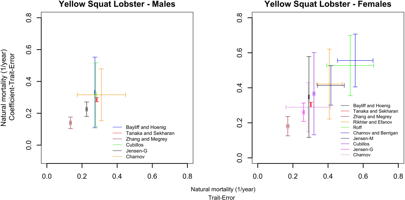
Fig. 2. Uncertainty of the natural mortality estimations (M) for males and females of yellow squat lobster (Cervimunida johni) considering trait-error and coefficient-trait-error. (Centre point corresponds to mean value of M estimate of each method and bars to the standard deviation).
Table 3. Natural mortality estimates (M, year−1) for yellow squat lobster, considering trait-error and coefficient-trait-error

CV, coefficient of variation of the M estimates.
Bold numbers indicate M estimators based on length. Italics indicate the estimator based on age at maturity (t m). LI, LS represent the lower and upper 95% confidence intervals respectively.
The estimated M for females across methods, considering trait-error, varied between 0.17 and 0.51 (year−1) and when coefficient-trait-error was considered (Table 3). The variability of M methods (CV) shows the same pattern as in male estimates, that is, CV was higher when body size was included in the estimation of M (Table 3). Unlike the male M estimations, for female methods based on t m (age at maturity) were considered. These M estimations were all higher in comparison with methods that excluded t m (Table 3), and both point or body size-based estimations. Additionally, the CVs of trait-error based M values, were higher regarding methods that did not include t m. The uncertainty of female M estimations varied widely depending on the method (Figure 2). Smallest uncertainty was associated with the same methods as for males.
Red squat lobster
Table 4 summarizes the M estimations for red squat lobsters in the northern and southern area. In general, M estimations for males and females of red squat lobster in the south were higher than M estimations in the north (Table 4).
Table 4. Natural mortality estimates (M, year−1) for red squat lobster, Northern stock (left) and Southern stock (right), considering trait-error and coefficient-trait-error

Bold numbers indicate M estimators based on length. Italics indicate the estimator based on age at maturity. LI, LS represent the lower and upper 95% confidence intervals of M respectively, CV, coefficient of variation of the M estimates.
North
Values of M for males based on trait-error and coefficient-trait-error ranged from 0.26 to 0.37 (year−1). Variability (CV) of the M estimates followed the same pattern as for yellow squat lobster (Table 3), for instance the method based on body size showed large variability (CV) and uncertainty (Table 4, Figure 3), as did Cubillos's estimator.

Fig. 3. Uncertainty of the natural mortality (M) for males and females of red squat lobster (Pleuroncodes monodon) considering the trait-error and coefficient-trait-error. (Centre point corresponds to mean value of M estimate of each method and bars to the standard deviation.)
The M estimations for females under trait-error or coefficient-trait-error varied between 0.24 and 0.45 (year−1) (Table 4). In general, median estimates of M using age at maturity (t m) showed higher values from those models that did not consider t m. Charnov and Berrigan's estimator generated the highest M estimates either with trait-error or coefficient-trait-error (Table 4). Variability (CV) of M showed the same pattern as males (Table 4) with higher estimates for methods using the maturity trait; however, M estimators based on t m showed a lower variability compared with, for instance, yellow squat lobster females. Figure 3 shows that the methods with the largest uncertainty corresponded to Bayliff and Hoenig's, and Cubillos's estimators.
South
Male estimations of M varied from 0.43 to 0.68 (year−1) for either the trait-error case or coefficient-trait-error (Table 4). Like previous cases, variability of M between methods showed the same pattern, higher CVs were associated with size dependent methods. Higher CVs across methods were also obtained when coefficient-trait-error was considered (Table 4). Cubillos's method yielded the highest M estimate for males in the southern area as well as uncertainty (Table 4, Figure 3). As in the previous cases, uncertainty was reduced if only trait-error was considered, with the exception of Charnov's estimator (Figure 3) being a size-based method.
Median M estimates for the females fluctuated between 0.41 and 1.06 (year−1) either for trait-error or coefficient error (Table 4). Like in the northern area, the M values based on models that considered age at maturity were higher compared with those based on size or t max (Table 4). Estimates of M were higher than the northern stock and varied widely between methods (Figure 3).
Discussion
We presented the first comprehensive analysis of natural mortality estimates for the main harvested squat lobster populations in Chile. A wide range of estimators were considered, with an extensive treatment of uncertainty incorporating both trait and coefficient errors. Brodziak et al. (Reference Brodziak, Ianelli, Lorenzen and Methot2011) and Hoenig et al. (Reference Hoenig, Then, Babcock, Hall, Hewitt and Hesp2016) recommended the comparison of indirect estimates of M with field-derived measurements of M, direct estimates of M are not available for both Chilean squat lobster species.
In an intra-species comparison, females showed larger estimates of M than males. Inter-stock differences were also observed, with red squat lobster (males and females) in the south showing larger M estimates than the estimated values for both the northern stock of red squat lobster and for the yellow squat lobster. High variability of uncertainty among indirect methods was described and it is related with M estimators using t max or t m and body size. This finding agreed with previous studies of M in species such as skate and pink cusk-eel reported by Quiroz et al. (Reference Quiroz, Wiff and Caneco2010) and Wiff et al. (Reference Wiff, Quiroz, Ojeda and Barrientos2011), respectively.
The large variability observed in the M estimates is associated, on one hand, with the type of indirect method used, which varied in the number of parameters used, their uncertainty and their theoretical backgrounds. For instance, Zhang & Megrey (Reference Zhang and Megrey2006) considered three life history parameters (k, t max and b), while Jensen (Reference Jensen1996) considered only the somatic growth rate k. Alternatively, the M estimator in Charnov et al. (Reference Charnov, Gislason and Pope2012) depends on two parameters and varied with body size (length). We observed that the functional forms of M methods that incorporate maturity lead to higher estimates of M compared with those that did not, explaining the notable differences in the case of females. A possible explanation for this might be early developing maturity of squat lobsters compared with their maximum longevity. Hutchings & Kuparinen (Reference Hutchings and Kuparinen2017) argued that declining size at maturity leads to an increase in mortality, mainly because M is significantly correlated with the maximum per capita population growth rate. It has been noted that among most of the life history parameters, reproductive traits have higher M predictive power (Gunderson & Dygert, Reference Gunderson and Dygert1988).
Bucarey (Reference Bucarey2015a) summarized yellow squat lobster M estimations between 1994 and 2000, using the indirect methods of Alagaraja (Reference Alagaraja1984) (in this study, the Tanaka–Sekharan estimator), Rikhter & Efanov (Reference Rikhter and Efanov1976) and Pauly (Reference Pauly1980). These estimates varied between 0.25 and 0.77 (year−1) for males and 0.165 and 0.99 (year−1) for females. In addition, the current gender-based M values used in the stock assessment were assumed fixed and estimates using Pauly's method with M values of 0.30 (year−1) for females and 0.25 (year−1) for males. Although some of these values can be located within the range of the M estimates found here, these ignored the uncertainty of M and used indirect methods that do not apply across taxa, so comparisons are difficult to establish. For instance, we did not include Pauly's method because it has no theoretical extension for crustaceans.
Regarding red squat lobster, Bucarey (Reference Bucarey2015b) summarized the M estimates from five indirect methods (Alverson & Carney, Reference Alverson and Carney1975; Rikhter & Efanov, Reference Rikhter and Efanov1976; Alagaraja, Reference Alagaraja1984; Roff, Reference Roff1984) that yielded an M range from 0.23 to 0.62 (year−1) for males and 0.21 to 0.75 (year−1) for females. Quiroz et al. (Reference Quiroz, Montenegro, Báez, Espíndola, Canales, Reyes, Magnere, Yáñez, Tapia, Bahamonde, Arriagada and Gálvez2006), using a variance-weighted method across different indirect approaches (Alverson & Carney, Reference Alverson and Carney1975; Rikhter & Efanov, Reference Rikhter and Efanov1976; Pauly, Reference Pauly1980; Hoenig, Reference Hoenig1983; Jensen, Reference Jensen1996) estimated M by sex for red squat lobsters inhabiting a smaller fraction of the northern area of the fishery, reporting values of 0.23 to 0.42 (year−1) for males and 0.17 to 0.31 (year−1) for females. Although comparisons of M estimates are difficult to establish, the M estimates of this work were closer to the M values reported by Quiroz et al. (Reference Quiroz, Montenegro, Báez, Espíndola, Canales, Reyes, Magnere, Yáñez, Tapia, Bahamonde, Arriagada and Gálvez2006).
In general, confidence intervals coming from trait-errors were smaller than those from coefficient-errors. This aspect is related to the nature of the estimated uncertainty in growth and maturity parameters (CV or standard error) in most crustacean species. For example, age assignment is usually conducted by counting rings in hard structures such as otoliths in teleost fish. Therefore, somatic growth is estimated using data comprising several observations of fish of the same age-class but different lengths. In such cases, uncertainty in growth parameters accounts for individual variability of the length at age, which then propagated into the estimation of M using indirect methods. Alternatively, pseudo-cohort age-assignment in crustaceans is usually done by modal decomposition of length structures (Macdonald & Pitcher, Reference Macdonald and Pitcher1979), due to the difficulties in using hard body parts for age determination (Kilada & Acuña, Reference Kilada and Acuña2015). Using this method ignores the variation in individual growth because length at age is only represented by the median length for each age group, except when a presumed length variation by pseudo-cohort has been incorporated. This way, growth parameters are estimated using one (or few) observations of length at age and therefore the uncertainty for growth parameters estimated from modal age decomposition is low. Thus, low uncertainty in growth parameters underestimates the uncertainty in trait-errors using indirect methods to estimate M.
Although uncertainty varied between methods due to reported or assumed uncertainty, it was also influenced by the type of probability distribution assumed (asymmetry) during the Monte Carlo re-sampling. Wiff et al. (Reference Wiff, Quiroz, Ojeda and Barrientos2011) mentioned that the asymmetry of the distribution responds to the multiplicative structure in logarithmic scales that in some models is assumed in the errors of the different coefficients that described the applied method. Therefore, the distribution of error in the M estimates is difficult to tackle analytically, because each parameter feeding the empirical models of M may have a particular distribution. Thus, we recommend to choose the most appropriate distribution for the parameters feeding the models to estimate M, and then work with the empirical (re-sampled) distribution of M. Note, this distribution for M may not be symmetrical, as a result of the error structure of feeding parameters and the manner of combining them in the chosen natural mortality estimator.
All methods presented here for crustaceans did not include environmental temperature in their equations, which seems counterintuitive. The effect of temperature on metabolic rates has a solid theoretical and empirical basis (Brown et al., Reference Brown, Gillooly, Allen, Savage and West2004). Natural mortality is shaped by intrinsic processes controlled by metabolic rates (i.e. reproduction), and therefore, environmental temperature should play an important role in estimating M. The nature of this problem is down to the way temperature seems to affect the intrinsic causes of natural mortality. Charnov & Gillooly (Reference Charnov and Gillooly2004) theorized that temperature, via metabolic rates, will affect directly maturity and senescence in indeterminate growers, so natural mortality should be indirectly affected by temperature. On the other hand, Gislason et al. (Reference Gislason, Niels, Rice and Pope2010) conducted a meta-analysis in teleost fishes demonstrating that temperature does not have a significant effect on natural mortality. Later, Charnov et al. (Reference Charnov, Gislason and Pope2012) generalized Gislason's theory showing that natural mortality in fishes is only determined by life history parameters. Although the relationship between environmental temperature and mortality has been studied almost exclusively in teleost fishes, we may hypothesize that the same rules should apply in the case of crustaceans; both taxa show indeterminate growth and natural mortality is shaped by intrinsic and extrinsic (e.g. predation) forces. Debate on the effect of environmental temperature on natural mortality still continues (Charnov & Gillooly, Reference Charnov and Gillooly2004; Gislason et al., Reference Gislason, Niels, Rice and Pope2010), and the proof of its effect can only be achieved by disentangling the intrinsic and extrinsic causes of mortality.
In the case of indirect M estimators, environmental temperature seems to affect the parameters that feed the models (e.g. maturity, longevity). We found that M estimates for red squat lobsters were different between areas (north and south) and this was consistent with the pattern of somatic growth of the red squat lobsters in both areas. Red squat lobsters in the north grow slowly compared with the south, and M estimates were lower in the north compared with the south regardless of the sex and consistent with life history theory. To explain the differences in somatic growth between areas, several hypotheses have been proposed that indicate a phenotypic response to habitat conditions. Differences in availability of food, hydrographic conditions (temperature), level discharge of fresh water and sedimentary material and differences in predation could explain differences in somatic growth (Roa & Tapia, Reference Roa and Tapia1998).
Overall, our analyses indicate that the M models are not comparable, at least not straightforwardly, which makes it challenging to select the most appropriate one. Previously, averaging M across methods has been done to account for the variability of M; however, that approach requires strong assumptions and has not been successful (Hamel, Reference Hamel2014; Hoenig et al., Reference Hoenig, Then, Babcock, Hall, Hewitt and Hesp2016). It assumes that all methods applied are equally good (or bad) which is nonsensical since the theoretical background of each method makes it more suitable for certain taxa/stock/regions and assumes that all methods have the same error distribution which is not the case in the applied estimators used here. Moreover, owing to the spectrum of methods that exist to estimate M in term of parameters used, information quality, and the large variability level of uncertainty it is difficult to recommend a single value, demonstrating that the indirect estimations of M are far from precise (Kenchington, Reference Kenchington2014). Thus, we would like to emphasize the need to propagate the uncertainty of M estimates into the stock assessment result and therefore management quantities (Brodziak et al., Reference Brodziak, Ianelli, Lorenzen and Methot2011). One method could be creating a combined prior for M in the stock assessment (Hamel, Reference Hamel2014), or alternatively run a sensitivity analysis including various methods of M estimations with different levels of uncertainty (Brodziak et al., Reference Brodziak, Ianelli, Lorenzen and Methot2011).
Acknowledgements
We are grateful to the anonymous Reviewers and the Editor who helped to improve this manuscript.
Financial support
This work was funded by Instituto de Fomento Pesquero (IFOP) – Chile in the context of the project ‘Evaluación directa de langostino amarillo y langostino colorado entre la II y VIII Región, año 2016.’ T.M. Canales was funded by the Fondecyt Post-Doctoral Project No. 3160248. R. Wiff was funded by the project CONICYT PIA/BASAL FB0002. J.C. Quiroz was awarded a Conicyt BECAS-CHILE scholarship from the Chilean Government and a Top-Up Flagship Postgraduate Scholarship from the University of Tasmania, Australia.


