


INTRODUCTION
Species richness, species relative abundances, and heterogeneity of their spatial or temporal distributions in a given area are the central subjects of community ecology (He & Legendre, Reference He and Legendre2002). Species richness is the simplest way to describe community and regional diversity (Magurran, Reference Magurran1988), however its measurement and comparison are still affected by recurrent pitfalls (Gotelli & Colwell, Reference Gotelli and Colwell2001). Communities may differ in measured species richness due to real differences in underlying species richness, to differences in the shape of the relative abundance distribution, or to differences in the number of individuals counted or collected (Denslow, Reference Denslow1995). Most of the studies in community ecology of marine habitats published in recent years have pretended to estimate species richness, however several of these studies have actually quantified species diversity as species density; the number of species per unit area (quadrants or swept area) (Gotelli & Colwell, Reference Gotelli and Colwell2001).
Diversity indices have been used recurrently to determine spatial and temporal variation induced by natural and anthropogenic disturbances, and there are numerous references that support this use, but a methodological procedure to find a desirable diversity level for management has not been derived from these papers. Because most diversity indices are sensitive to both evenness and richness, differences can reflect changes in either or both; and changes in evenness should not be interpreted as changes in richness (Levin et al., Reference Levin, Etter, Rex, Gooday, Smith, Pineda, Stuart, Hessler and Pawson2001). In fact, the selection of the most adequate indices is not in the most cases the substantial goal in the search for disturbance evidence, because most of the indices are supported by complex or cryptic concepts and generally they could be correlated (see Washington, Reference Washington1984).
There is now strong evidence that commercial fishing has a profound effect on marine ecosystems (Jennings & Kaiser, Reference Jennings and Kaiser1998; Hall, Reference Hall1999; Kaiser & de Groot, Reference Kaiser and de Groot2000; Thrush & Dayton, Reference Thrush and Dayton2002), however a lack of environmental-impact assessment procedures in fishing management still persists (Thrush et al., Reference Thrush, Hewitt, Cummings, Dayton, Cryer, Turner, Funnell, Budd, Milburn and Wilkinson1998). Recently there have been great improvements in our understanding of community level changes in response to fishing (Hall, Reference Hall1999), and species diversity has been considered as a primary factor for management of multispecies fisheries. In contrast, nowadays there are few tropical regions where the soft-bottom species richness have been adequately inventoried and accurate richness levels for conservation have been established (Levin et al., Reference Levin, Etter, Rex, Gooday, Smith, Pineda, Stuart, Hessler and Pawson2001; Gray, Reference Gray2002). Basic patterns, as natural seasonal changes of species diversity and their relation with the depth gradient at local and regional scales remain unknown, impeding the identification and potential impact of disturbance forces (natural and anthropogenic) that structure the communities (Godínez-Dominguez et al., unpublished data). Natural systems have a great deal of structure in time and space, and it is important to identify thresholds of change in this structure and the processes involved to gauge ecosystem resilience (Thrush & Dayton, Reference Thrush and Dayton2002).
Spatiotemporal variation in benthic species diversity represents the integration of ecological and evolutionary processes that operate at different spatial and temporal scales (Levin et al., Reference Levin, Etter, Rex, Gooday, Smith, Pineda, Stuart, Hessler and Pawson2001), and if we want to understand diversity, we should look for mechanisms that influence the abundances and spatial distribution of species (He & Legendre, Reference He and Legendre2002). Here, diversity of the soft-bottom macroinvertebrate assemblage inhabiting the Mexican central Pacific is analytically decomposed using estimates of richness, evenness and species density. These measures could explain the basic and conspicuous structural traits of the macroinvertebrate diversity. The relations among the diversity and spatial and temporal environmental variability were modelled. Finally we discuss the relationships of the results obtained with the survey scale and their management implications.
MATERIALS AND METHODS
Sampling
The study area is located on the continental shelf in the Mexican central Pacific (Figure 1), between the 10 and 90 m isobaths, from Punta Farallón (Jalisco) to the mouth of the Cuitzmala River to Cuyutlán (Colima). The continental shelf of this region is very narrow, comprising, up to the 200-m isobath, only 7–10 km (Filonov et al., Reference Filonov, Tereshchenko, Monzon, González-Ruelas and Godínez-Domínguez2000). The predominant surface current in the study area is linked to the current pattern described by Wyrtki (Reference Wyrtki1965) for the eastern Pacific Ocean, consisting of the two main phases: the first one is influenced by the California Current, and it is characterized by a cold water mass from January–February to April–May; the second phase (July–August to November–December) is influenced by the North Equatorial Countercurrent and characterized by a tropical water mass. A transition phase is usually recognized during which none of the previous phases dominates. This hydroclimatic seasonality is the most influent force that determines the temporal patterns of the macroinvertebrate community in the zone (Godínez-Domínguez, Reference Godínez-Domínguez2003).
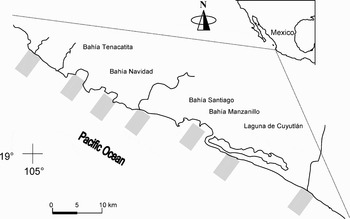
Fig. 1. Study area. Rectangles indicate sampling sites.
Five cruises (DEM 1 to DEM 5) were conducted aboard the RV ‘BIP-V’ during the different hydroclimatic seasons: May–June (transition; DEM 1) and November–December (tropical; DEM 2) 1995, and March (subtropical; DEM 3), June (transition; DEM 4) and December (tropical; DEM 5) 1996. Samples were collected at night with a double otter trawl (one on each side of the boat) similar to those used in the commercial shrimp fisheries in the Mexican Pacific but with reduced mouth size (6.9 m width) and mesh size (38 mm in the cod end). Seven sites were selected along the coast according to the spatial distribution of soft bottoms and the fishing grounds mostly visited by the commercial fleet. Four depth strata were selected (20, 40, 60 and 80 m) for each site making a total of 28 sampling stations per cruise. Each tow lasted 30 minutes at 2 knots speed corresponding to an average of one hectare trawled by sampling station. The sampling order of the sites was randomly selected. Samples from a same site were taken the same night in a random way, preserved on ice and processed immediately. Organisms of all macroinvertebrate groups (cnidarians, molluscs, crustaceans and echinoderms) were identified taxonomically and counted, and the fresh weight by species was recorded.
Diversity estimates for each cruise were calculated per depth strata, and the seven sampling sites were considered as replicates. Evenness and species richness were estimated using two null models. Evenness was estimated using the probability of an interspecific encounter PIE (Hurlbert, Reference Hurlbert1971):
where N is equal to the total number of individuals in the collection, and S is the total number of species in the collection and mi is the number of individuals of species i in the collection. This index gives the probability that two randomly sampled individuals from the assemblage represent two different species, and it is characterized by two main attributes: it is easily interpreted as a probability, and it is one of the few indices that is unbiased by sample size, although variance increases with small N (Gotelli & Entsminger, Reference Gotelli and Entsminger2001).
Species richness was estimated using rarefaction curves (Gotelli & Graves, Reference Gotelli and Graves1996), which generate comparative estimates of species number independently of the differences in sampling sizes of the groups compared. An individual-based procedure was used in the rarefaction estimation. The abundance levels for simulations were established using the sample with the lowest abundance (700 organisms) to allow the comparison between expected richness and evenness among the samples. Both evenness and rarefaction were estimated using EcoSim software (Gotelli & Entsminger, Reference Gotelli and Entsminger2001), which uses a Monte Carlo procedure, and 1000 replicate simulations were performed for each estimate. Samples are drawn randomly without replacement, and the procedure is repeated 1000 times to estimate an average value and confidence interval (95%) at several abundance levels.
The species–area curve (Rosenzweig, Reference Rosenzweig1995) was used as a species density index:
where S is the species richness, A the trawled area, the intercept a is related to overall species richness and the slope β constitutes an index of species density.
Generalized linear models (GLM) were employed to determine the relations between indices of diversity (species richness and evenness) and the slope of species–area curves, environmental spatiotemporal factors (season and depth), and organism abundance (local: average per depth strata, and regional: average for the complete sampling area per cruise). A normal log model was assumed, and the best subset procedure based on the Akaike information criterion (AIC) was used to select the most parsimonious model.
RESULTS
A marked temporal trend in species richness was observed throughout the study period (Figure 2). The highest richness was observed during the DEM 1 cruise declining gradually toward the last cruise, 2 years later. A similar richness–depth pattern was observed in the DEM 1 and 4 cruises; with a higher number of species observed in shallow (20 and 40 m) than in deep waters (60 and 80 m). In shallow waters the average species richness was 45 and 25 (expected number of species) in DEM 1 and DEM 4 respectively, whereas in deepest waters the expected richness was 33 and 15. Cruises DEM 1 and 4 were carried out in the same hydroclimatic season (transition between tropical and subtropical period), and a similar bathymetric pattern of assemblage organization has been reported elsewhere (Godínez-Domínguez et al., unpublished data). Cruises DEM 2 and 5 were carried out in the tropical period but they showed a different richness–depth pattern. During Cruise DEM 2 the highest richness was estimated in the shallowest stratum (20 m, 34 species), while in DEM 5 the overlapping of the confidence intervals indicate similar richness among strata (range: 11–18 species). Cruise DEM 3 (subtropical season) showed a similar richness in the different depth strata ranging from 24 to 30 species. The distribution along the depth gradient of the macroinvertebrate assemblages (described in Godínez-Domínguez et al., unpublished data) was similar in cruises DEM 2, 3 and 5, and in all cases different assemblages characterized each of one of the depth strata.
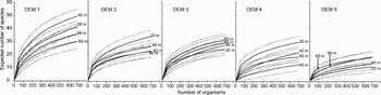
Fig. 2. Rarefaction curves of the macroinvertebrate assemblages for each cruise and depth strata. Solid lines are average of the richness estimates; dotted lines are the 95% confidence intervals. Cruise DEM 1 (May–June 1995), DEM 2 (November–December 1995), DEM 3 (March 1996), DEM 4 (June 1996) and DEM 5 (December 1996).
No temporal trend could be detected in evenness (Figure 3). The highest PIE values in DEM 1 and 4 (transition period) were obtained at 20 m (0.88 and 0.84, respectively). In tropical seasons (DEM 2 and 5) evenness and depth showed contrasting patterns: while in DEM 5 evenness increased with depth, it decreased in DEM 2. In DEM 3, PIE values were generally high and fluctuated in a narrow range of 0.64 to 0.80. No time trends were observed in the slope of the species–area curves (Figure 4). However a general inverse trend in relation with depth could be observed and two groups (shallow, 20 and 40 m; deep 60 and 80 m) of slope values could be discriminated. Correlation among diversity indices and local abundance was estimated. Species richness and evenness showed a positive correlation (P < 0.05) (Figure 5), while the species–area slope did not show significant (P > 0.05) relations with richness or evenness. Abundance only showed a significant negative correlation with the evenness.
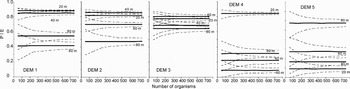
Fig. 3. Evenness (probability of an interspecific encounter) estimated for each cruise and depth strata of the macroinvertebrate assemblages. Solid lines are average of the richness estimates; dotted lines are the 95% confidence intervals.
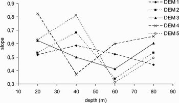
Fig. 4. Slopes of species–area curves estimated for each cruise and depth strata.
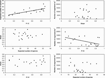
Fig. 5. Relationship among the different diversity indices and local abundance. Linear regressions are shown for significant relationships (P < 0.05).
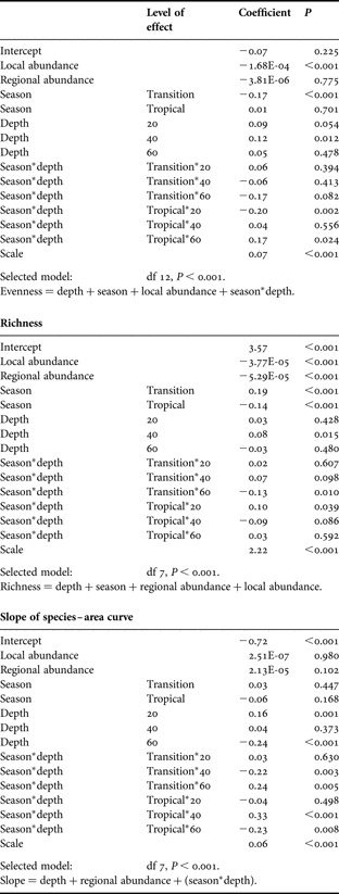
The model selected for evenness using GLM included the environmental variables (depth, season and their interaction) and local abundance (Table 1). The best model for species richness included abundance estimates, seasonality and depth but not their interaction. The most parsimonious model explaining the slope of the species–area curve included regional abundance, depth and the season–depth interaction. Only depth was included as independent variable in all the models fitted. From the analysis of the GLM coefficients, a decrease in evenness was detected during the transition. The shallow strata (20 and 40 m) showed highest evenness values, while increases in local abundance were associated with decreases in evenness. The species richness attained a minimum during the tropical period and a maximum in the transition. The richness at 40 m was higher than in other depth strata, while the relation with the regional abundance was negative. The slope of species–area curve shows a positive relation with the regional abundance, and it is lower at 60 m than in other depths. The AIC procedure of model construction considers variables that individually could be statistically significant or not, and for this reason there are variables that showed significant fits but were not selected in the most parsimonious model as in the slope model; on the other hand, there are variables with non-significant individual fits that were included in the most parsimonious models (see Table 1).
Table 1. Parameters of models relating diversity indices (species richness, evenness, slope of species–area curves) with environmental variables (depth, season) and abundance (local and regional). Selected model is the most parsimonious model (GLM) according to Akaike information criterion (AIC).
DISCUSSION
The standardization of an area or sampling effort may produce very different results compared to standardizing by number of individuals collected. Rarefaction methods used with both sample-based and individual-based procedures could produce contradictory results, and these differences could be explained by spatial patchiness patterns (Gotelli & Colwell, Reference Gotelli and Colwell2001). We have used a fixed number of organisms determined by the lowest sample size (700 organisms) to calculate species richness and evenness with the individual-based procedure, according to Gotelli & Colwell (Reference Gotelli and Colwell2001) and Levin et al. (Reference Levin, Etter, Rex, Gooday, Smith, Pineda, Stuart, Hessler and Pawson2001), to allow for comparisons. The PIE evenness index is unbiased by sample size but comparisons of species richness are affected by abundance (Rosenzweig, Reference Rosenzweig1995). For this reason it is important to use the species accumulation curve to quantify taxon richness, even in studies in which sampling effort is carefully standardized (Gotelli & Colwell Reference Gotelli and Colwell2001), as in the present case.
The declining trend of species richness observed in the present study could be related to the cumulative effects of interannual environmental variability and fishing disturbance. This study was carried out previous to the most important El Niño event (1997–1998) of the 20th Century (Philander, Reference Philander1999), and a fishing-induced state of chronic disturbance has been reported in this community (Godínez-Domínguez et al., unpublished data). The ENSO effects in the benthic communities remain unknown. Trawling on soft-bottoms produces disturbances at several scales, modifying habitat structure and inducing sediment homogenization (Jennings & Kaiser Reference Jennings and Kaiser1998; Thrush & Dayton Reference Thrush and Dayton2002), thus affecting biodiversity at broad-scales. Besides it is not possible to discriminate disturbance sources (anthropogenic and natural) in the benthic community studied, and environmental disturbances such as interannual variability could be more influent than impact due to fishing (Godínez-Domínguez et al., unpublished data).
Disturbance regimes play a key role in influencing biodiversity (Connell, Reference Connell1978). Although the fishing effort in most fisheries is non-evenly distributed in space, fishing impacts are perceived at a broad or regional scale (Kaiser & Spencer, Reference Kaiser and Spencer1996; Thrush et al., Reference Thrush, Hewitt, Cummings, Dayton, Cryer, Turner, Funnell, Budd, Milburn and Wilkinson1998). Fishing disturbance and recovery time depend on species, type of gear, habitat and frequency of disturbance (Collie et al., Reference Collie, Hall, Kaiser and Poiner2000). Often the scales of measurement of fishing effort do not match well with scales of variability in seafloor ecological communities (Thrush & Dayton, Reference Thrush and Dayton2002). Studies aimed at explaining the relation between fishing disturbance and biodiversity, differ in their conclusions related to the assemblage response (Kaiser & Spencer Reference Kaiser and Spencer1996; Kaiser et al., Reference Kaiser, Armstrong, Dare and Flatt1998; Thrush et al., Reference Thrush, Hewitt, Cummings, Dayton, Cryer, Turner, Funnell, Budd, Milburn and Wilkinson1998; Tuck et al., Reference Tuck, Hall, Robertson, Armstrong and Basford1998; Pranovi et al., Reference Pranovi, Raicevich, Franceschini, Farrace and Giovanardi2000; Sánchez et al., Reference Sanchez, Demestre, Ramon and Kaiser2000; Veale et al., Reference Veale, Hill, Hawkins and Brand2000), and this inconsistency could be attributed to the method used for measuring diversity (species richness, diversity indices, species density, abundance and composition), lacking of an a priori hypothesis, and confounding the scale of the surveys.
Bathymetric patterns in evenness and species richness are variable in different DEM cruises and within the same hydroclimatic season. Although evenness and richness showed a strong correlation, species richness could be a better indicator of temporal variability. The species–area relationship could be considered a better indicator of spatial heterogeneity specifically to illustrate the depth gradient. Evenness is related to abundance variability as indicated by their high correlation. According to Thrush et al. (Reference Thrush, Hewitt, Funnell, Cummings, Ellis, Schultz, Tallet and Norkko2001) diversity components could be related with scale and the relative importance of physical and biological elements of habitat structure vary with spatial scale. Two main relationships are deduced from most previous studies focused on the estimation of diversity of demersal fish and macrobenthic communities associated with soft-bottom: diversity–depth (Bianchi, Reference Bianchi1991; Coleman et al., Reference Coleman, Gason and Poore1997; Gray et al., Reference Gray, Poore, Ugland, Wilson, Olsgard and Johannessen1997) and diversity–scale (Thrush et al., Reference Thrush, Hewitt, Funnell, Cummings, Ellis, Schultz, Tallet and Norkko2001; Thrush & Dayton, Reference Thrush and Dayton2002). Despite that the richness–depth relation in soft-bottom communities has been a topic widely reviewed (Grassle & Maciolek, Reference Grassle and Maciolek1992; Gray, Reference Gray1994, Reference Gray2002; Coleman et al., Reference Coleman, Gason and Poore1997; Levin et al., Reference Levin, Etter, Rex, Gooday, Smith, Pineda, Stuart, Hessler and Pawson2001) there is still a controversy about conceptual and methodological aspects of the relationship along the latitudinal and depth gradients, although there is some coincidence that the model that better explains the response of the diversity to these gradients could be unimodal (Levin et al., Reference Levin, Etter, Rex, Gooday, Smith, Pineda, Stuart, Hessler and Pawson2001; Gray, Reference Gray2002), at least for depth in some taxonomic groups. Of course this unimodal gradient is evidenced only when a large depth-range is analysed. Actually, the depth–diversity relationship is contained in the diversity–scale relationship, and most of the controversy derived from the depth–diversity relationship is due to differences in scale of the surveys, sampling effort and numerical procedures to estimate diversity (Levin et al., Reference Levin, Etter, Rex, Gooday, Smith, Pineda, Stuart, Hessler and Pawson2001; Gray, Reference Gray2002).
Rosenzweig (Reference Rosenzweig1995) suggested that the number of species in an area was likely related to habitat richness of that area, since areas of greater richness offer new niches for colonizing species. Therefore areas with greater habitat richness should have more species per unit area, resulting in steeper slopes of the species–area curves. The hypothesis that habitat richness decreases with depth appears reasonable even in a short depth gradient (in our case 10–90 m). The inshore zone (including sheltered and exposed areas) in tropical latitudes constitutes nurseries (Blaber & Blaber, Reference Blaber and Blaber1981) and it is recognized as ecologically conspicuous and containing diverse habitats (Longhurst & Pauly, Reference Longhurst and Pauly1987). The interior shelf is characterized by high-energy flows, tidal cycles and current patterns that cause a dynamic water column (Darnell, Reference Darnell1990), and could be related with the high heterogeneity and dynamics of the seabed. The ‘habitat diversity hypothesis’ (Anderson, Reference Anderson1998) is probably the better conceptual model proposed to explain the ecological or statistical processes underlying the species–area relationship in the tropical Pacific shelf.
The inverse relation between evenness and abundance is a topic widely studied and could represent an ecological feature of the community studied; increases in abundance are due to an increase in the dominance of a few species and states of high abundance with high evenness are not a frequent situation. According to He & Legendre (Reference He and Legendre2002), if a mechanism can make the species abundances more even, or their spatial distribution more regular, this factor should contribute to species coexistence, and vice versa. In communities with high dominance sub-estimation of species richness is more probable due to the high number of organisms needed to find new species, and for this reason, sampling deficiencies in these communities are expected more frequently.
The coupling between diversity and assemblage patterns (described by Godínez-Domínguez & Freire, Reference Godínez-Domínguez and Freire2003) has not been appreciated. Changes in assemblage structure are not always followed by diversity changes at the same scale (Gray, Reference Gray2003). Assemblages can vary within small depth-ranges (Bergen et al., Reference Bergen, Weisberg, Smith, Cadien, Dalkey, Montagne, Stull, Velarde and Ranasinghe2001; Godínez-Domínguez & Freire, Reference Godínez-Domínguez and Freire2003) but species richness changes over larger scales (Rex et al., Reference Rex, Stuart, Hessler, Allen, Sanders and Wilson1993, Reference Rex, Stuart and Coyne2000; Gray et al., Reference Gray, Poore, Ugland, Wilson, Olsgard and Johannessen1997). This could be the reason why several analyses cannot reconcile results from multivariate ordinations of assemblage matrices and diversity indices estimates at the same scale. These results force usually the search for more ‘sensitive’ indices trying to reconcile patterns when the real problem is related to scale.
We made tows of 1 ha at each depth and small-scale heterogeneity was not considered in the data, but this level of heterogeneity is not relevant to account for diversity at broad scales (the fisheries scale) or when the depth–diversity relationship is analysed. However, in marine benthic habitats small-scale natural disturbances play an important role influencing communities by generating patchiness (Sousa, Reference Sousa1984; Dayton, Reference Dayton, Giller, Hildrew and Raffaelli1994; Hall et al., Reference Hall, Raffaelli, Thrush, Giller, Hildrew and Rafaelli1994), and heterogeneity is an important component of the functioning of ecological systems (Kolasa & Pickett, Reference Kolasa and Pickett1991; Legendre, Reference Legendre1993) and has implications for the maintenance of diversity and stability at the population, community and ecosystem levels. In soft-bottom habitats the creation of small-scale habitat structure by biogenic features can play key roles in influencing diversity and resilience (Thrush & Dayton, Reference Thrush and Dayton2002). In most of the fishing-disturbance surveys, several patchings are crossed in each sampling tow and this heterogeneity level only could be reflected in a ratio variance/mean. Species within a local assemblage (1–10 m2) are controlled by small-scale processes involving resource partitioning, competitive exclusion, predation, facilitation, physical disturbance, recruitment, and physiological tolerances, all of which are mediated by the nature and degree of heterogeneity (Levin et al., Reference Levin, Etter, Rex, Gooday, Smith, Pineda, Stuart, Hessler and Pawson2001). At regional scales (100s to 1000s of m), several environmental gradients, dispersal, metapopulation dynamics, and gradients in habitat heterogeneity are likely to be important (Levin et al., Reference Levin, Etter, Rex, Gooday, Smith, Pineda, Stuart, Hessler and Pawson2001).
ACKNOWLEDGEMENTS
This research was partially founded by the University of Guadalajara and the Consejo Nacional de Ciencia y Tecnología CONACyT Mexico, and by the grant REN2000-0446 from the Spanish Ministerio de Ciencia y Tecnología. We thank the RV ‘BIP-V’ crew and the ‘Demersales project’ staff for their help during the field phase and to Victor Landa Jaime, Rafael García de Quevedo Machaín, and Judith Arciniega Flores for taxonomic support.


