AMO/NAO and Bay of Biscay secular SST (1854–2010)

Figure 2A shows a time-series of the Atlantic Multidecadal Oscillation (AMO) index during the last 155 years (1856–2010). To compute the index, CDC uses the Kaplan SST dataset (5° × 5°) over the central North Atlantic (0–75°N 10–75°W), which calculates an area weighted average and removes the linear trend (Enfield et al., Reference Enfield and Cid-Serrano2001). The purpose of detrending is trying to eliminate the influence of the anthropogenic global warming. The Figure also presents the time-series of monthly SST anomalies (Figure 2B) in the Bay of Biscay region (44–48°N 2–10°W) for the same period (1854–2010). The AMO time-series (see Figure 2A) shows two long-term warming–cooling cycles comparable to those observed in the SST anomalies and described in the regional literature (Table 1). There are SST anomaly maxima near 1870 and 1950 and minima near 1900 and 1980 indicating a period of 60–80 years. The polynomial tendency line of the Biscay SST anomalies is similar to that of AMO but sloping up during the last 100 years since only the climate index was linearly detrended.

Fig. 2. (A) Time-series of the Atlantic Multidecadal Oscillation (AMO) Index from 1856 to 2010; (B) sea surface temperature (SST) anomaly (°C); (C) SST (°C) over the whole Bay of Biscay during the period 1854–2010. Monthly values. The values of SST anomaly and SST represent the mean of 15 points of 2° latitude/longitude resolution over the region 44–48°N 2–10°W. A 12-month running mean has been applied to the time-series of SST anomaly and SST to remove the seasonal variability. A polynomial tendency line of order 6 is presented in the three frames. The tendency line explains 20–25% (R²:0.22) of the monthly SST anomalies and 50% (R²:0.50) of annual SST anomalies of the Bay of Biscay. The highest monthly anomalies took place in September 1949 (+1.81 °C) and June 2006 (+1.67 °C) and the lowest in July and August 1912 (−1.85 ° C and − 1.81 °C).

Time-series of annual NAO, autumn NAO and winter NAO (1850–2000) are presented in Figure 3. Figure 4 presents the regression lines and the correlation coefficients of AMO and the different NAO indices against the SST anomalies (1856–2000/2010). Negative values of NAO during autumn have been related to the occurrence of the poleward current off northern Spain. Figure 5 shows for example a recent observation of the poleward current entering the Biscay region in 2009/2010 during a period of sustained negative NAO conditions (October 2009: –1.03, November 2009: –0.02, December 2009: –1.93, January 2010: –1.11, February 2010: –1.98, March 2010: –0.88). Atmospheric teleconnections developing southerly winds, such as the negative phase of NAO, will be in general associated during autumn and winter with the northward development of this current along the Iberian slopes. Negative values of NAO during November, December and January (winter NAO) have also been associated with a lag to decreases in the North Atlantic circulation in time-series of NAO and altimeter data (Pingree, Reference Pingree2002). The correlations of Figure 4 analyse both NAO and AMO and indicate that AMO explains ~25% of the interannual variability of the annual SST anomaly (R²: 0.24). Annual NAO, autumn NAO and winter NAO explain however ≤1% of the variability (R²: 0.003, R²: 0.005 and R²: 0.01 respectively). AMO is therefore a major long-term climate influence in the temperature of the Bay of Biscay during the last 150 years while NAO, a higher frequency climate oscillation, exerts some control over specific years with extreme changes

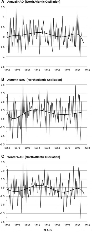
Fig. 3. Time-series of different North Atlantic Oscillation (NAO) indices during the period 1850–2000 (151 years): (A) annual NAO; (B) autumn NAO; (C) winter NAO. Annual values. In the three frames (A–C) a polynomial tendency line of order 6 is presented. Autumn NAO represents the November through December index. Winter NAO annual values are used here as in Pingree (Reference Pingree2002) (the November through January index). Hurrell (1995) defines Winter NAO as the December through March index. NAO is a high frequency climate index but some multidecadal variability can be observed in the tendency lines. Winter NAO for example shows minima near 1870 and 1960 (90 years) and maxima near 1910 and 1990 (80 years) pointing to a ~80 year cycle (see also Leterme & Pingree, 2007). This tendency line or long period variability explains however less than 5% of the data.

Fig. 4. Regression analyses and correlation coefficients of sea surface temperature (SST) anomaly (°C) in the Bay of Biscay (44–48°N 2–10°W; annual values) against: (A) Atlantic Multidecadal Oscillation (AMO) (Enfield et al., 2001) and different indices of North Atlantic Oscillation (NAO): (B) annual NAO; (C) autumn NAO; (D) winter NAO. The relationship between annual SST and annual SST anomalies in the Bay of Biscay for the region considered (44–48°N 2–10°W) is: SST = SSTa + 14.49. AMO can explain ~25% of the interannual variability of the SST anomaly (R²: 0.246) while annual NAO, autumn NAO and winter NAO explain ≤ 1% (R²; 0.003, R²; 0.005 and R²; 0.011 respectively).

Fig. 5. Thermal infra-red satellite images (AVHRR channel 4) showing the poleward current along northern Spain during the winter 2009/2010: (A) 25 December 2009 (13:42 GMT; NOAA-19); (B) 3 February 2010 (01:57 GMT; NOAA-19). Autumn–winter 2009/2010 was a period of strong and sustained negative North Atlantic Oscillation conditions (October 2009: –1.03, November 2009: –0.02, December 2009: –1.93, January 2010: –1.11, February: –1.98, March: –0.88). The images show some swoddies or Slope Water Oceanic eDDIES being formed from near Cap Ortegal (O10), Cap Breton canyon (B10), Cap Ferret canyon (F10), La Rochelle canyon (R10) and Aviles canyon (A10).

Other atmospheric teleconnections (1950–2010)

Table 2 shows a correlation matrix of the SST of the Bay of Biscay against the different atmospheric modes of the North Atlantic during a shorter period (1950–2010). The atmospheric modes analysed include in addition to NAO, EA, EA/WR, TNH, POL and SCA. Seasonal maps of these atmospheric patterns are shown in Figure 6. The correlation matrix (see Table 2) shows the influence of the EA and SCA teleconnections that explain respectively ~25% and ~20% (R²: 0.24 and R²: 0.19) of the interannual variability of the SST of the Bay of Biscay. AMO index has been included in the Table for comparison. Over the same 60 year period AMO accounts for ~40% (R²: 0.39) of the SST variability.

Fig. 6. Atmospheric teleconnections in the North Atlantic region (20° to 90°N): North Atlantic Oscillation (NAO), East Atlantic (EA) pattern, East Atlantic/Western Russia (EA/WR) pattern, Tropical/Northern Hemisphere (TNH) pattern, Polar/Eurasia (POL) pattern and Scandinavia (SCA) pattern. A teleconnection is a persistent and recurring pattern of pressure and circulation anomalies extending over a vast geographical region. They can be responsible for weather patterns occurring simultaneously over large distances. Source: NOAA Climate Prediction Centre (CPC; http://www.cpc.noaa.gov/data/teledoc/ telecontents.shtml). CPC isolates the primary teleconnection patterns from monthly 500 mb height anomaly maps and uses the Rotated Principal Component Analysis (RPCA) to calculate the monthly indices. The plots, elaborated at CPC, represent the temporal correlation during 1950–2000 between the monthly anomaly maps (for the three month period centred in January, April, July and October) and the index time-series for that month. The atmospheric teleconnections have a seasonal variation and some of them do not appear in all the months. The North Atlantic Oscillation (NAO) is the principal atmospheric mode of the North Atlantic where it explains 32% of the atmospheric variability (Cayan, Reference Cayan1992).

Table 2. Matrix of correlations (R²) of different North Atlantic atmospheric modes and sea surface temperature (SST, °C) in the Bay of Biscay during the period 1950–2010 (60 years). NAO, North Atlantic Oscillation; EA, East Atlantic pattern; EA/WR, East Atlantic/Western Russia pattern; SCA, Scandinavia pattern; TNH, Tropical/Northern Hemisphere pattern; POL, Polar/Eurasia pattern. Figure 6 shows maps of these atmospheric teleconnections. The Atlantic Multidecadal Oscillation (AMO) (an ocean climate index) has been included for comparison. The Climate Diagnostic Centre applies a 121 month smoother to the initial AMO index to obtain the smoothed AMO index.

AMO is an oceanic index based on SST and so it is likely to contain the influence of the atmospheric processes. Table 2 shows that the atmospheric modes NAO, EA, EA/WR and SCA explain each one 10–15% of the variance of the AMO index (R²: 0.15, R²: 0.13, R²: 0.14 and R²: 0.10 respectively). The correlations decrease against the smoothed AMO index (2–3%; R²: 0.03, R²: 0.03, R²: 0.02 and R²: 0.03 respectively) indicating that the variance explained by these atmospheric pressure modes (10–15%) is mainly contained in the high frequency fraction of the AMO values. A similar percentage of high frequency variance can be derived from the different correlations of the unsmoothed and smoothed AMO indices against the annual SST of the Bay of Biscay. The SST variability explained by AMO is reduced from ~40% (R²: 0.39) to 25–30% (R²: 0.27) after smoothing. The correlation between the smoothed and the unsmoothed AMO is R²: 0.62 which indicates that ~62% of the initial variance of the AMO values is contained in periods longer than 10 years. CPC applies a 121 months smoother to AMO. AMO represents therefore, even unsmoothed, a mode of decadal to multidecadal (D2M) climate variability.

Abrupt change of NAO and North Atlantic SST and circulation

NAO explains a very small percentage of the annual variability of the SST (see Table 2; Figure 4) but its influence can be realized through the accumulation of the climate anomalies. In connection with this, we have observed that the amount of variability explained in the long-term SST record (1854–2000) increases to 11%, 14% and 10% in the correlations made against cumulative annual NAO, cumulative autumn NAO and cumulative winter NAO respectively (R²: 0.11, R²: 0.14 and R²: 0.10). The importance and large-scale influence of NAO is also overwhelming during periods of strongly changing NAO conditions. Figure 7A shows for example the change of SST from January 1995 to January 1998 in the North Atlantic following the large change in NAO from positive winter (1993/1994/1995) to negative (1995/1996/1997) conditions. The period can be considered as representing a fall in North Atlantic Ocean circulation state (less anticyclonic) resulting from a positive to negative change in NAO or decreasing North Atlantic westerlies.

Fig. 7. (A) Temperature anomaly (°C) in January 1998 (after a period of negative North Atlantic Oscillation (NAO)) with respect to January 1995 (after several years of positive winter NAO). GS, Gulf Stream; NAC, North Atlantic Current; AC Azores Current; CC, Canary Current; (B) sea level change (cm) from January 1995 to January 1998 corresponding to the temperature anomalies of frame A. The results show that the longer term response to an abruptly decreasing step (1995/1996) in NAO is a tripole sea level anomaly structure (SPP), subpolar pole or polar pole; (C) central North Atlantic pole, but to the west of the Mid-Atlantic Ridge or with centre in the Western Basin; STP, Subtropical Gyre or North Equatorial Current region pole.

Following the winter NAO changes, January 1995 showed the SST region near the Azores to be warmer than the two regions to north (~+2°C) and south (~+1.5°C). For December 1995, a low sea level pressure is situated over the northern North Atlantic with associated cyclonic wind stress curl, Ekman transports and upwelling. In January 1996, SST was cooler by ~2°C in the Azores region and March 1996 showed the North Atlantic SST minimum near the Azores to be ~1.5°C cooler than the two positive anomaly maxima to the north and south consistent with a 1995/1996 fall in winter NAO. The developing or evolving SST situation is highly variable depending on the wind and seasonal heat flux forcing. A relative positive anomaly (~1°C) developed near the Azores in October and November 1996. A broad region of the North Atlantic Current lagged the 1995/1996 NAO decrease by about ~ 6 months (Pingree, Reference Pingree2005). The net effect of atmospheric forcing between January 1995 and 1998 coupled with the reduced circulation appeared to be a fall of SST of ~–1.0°C in the central region with less warm water from the Gulf Stream (Figure 7A). SST anomalies are >1.0°C south of Greenland indicating less southward flow of cold subpolar waters (under conditions with more easterly winds or less intense cold continental polar wind). The positive anomaly of >1.0°C emanating from the Canary Islands indicates a weaker Canary Current (cold) extension and westward North Equatorial Current (NEC). Global warming over the period is about 0.1°C (see Figure 2).

The large scale temperature anomalies of Figure 7A are related to a weakening anticyclonic North Atlantic Gyre as can be observed in the associated sea level anomalies derived from altimeter data (Figure 7B). For the North Atlantic altimeter change, it was necessary first to smooth the altimeter data (supplied by AVISO, CLS at 1/4 degree intervals, over the period 1992 to 2001) with a (5°×5°) latitude by longitude grid to reduce the eddy signal and for convenience filter the resulting time-series at each position to remove the seasonal or annual signal. Sea level over the same period (January 1995 to January 1998) falls (i.e. a cyclonic tendency for the geostrophic current) in the Gulf Stream Recirculation region (–8 cm change) which becomes less anticyclonic and also in the North Atlantic Current region (–10 cm change) resulting (geostrophically) in a weakened North Atlantic Gyre. A compensated rise in sea level occurs in the subpolar (+7) and subtropical region (+5). The geostrophic sense to the sea level slope is anticlockwise between these maxima with poleward tendency oceanward of the Iberian Peninsula (see Figure 7A). The results show that the longer term response to an abruptly decreasing step (1995/1996) in NAO is a tripole sea level anomaly structure (or quadrupole deformation since the negative or minimum region is more intense than the 2 elevated regions). The surface geostrophic flow has become more westerly near 50°N and less westerly near 27°N in the central North Atlantic ~40°W. The overall changes in sea level are much larger than the general rise of sea level over the period (from January 1995 to January 1998) which is ~+1 cm. Garcia-Soto et al. (Reference Garcia-Soto, Pingree and Valdés2002) showed continental slope warming in January 1996 and January 1998 and sea level set-up across the Bay of Biscay from altimeter data was found to come in two pulses centred near January 1996 and November 1997. The Iberian/Biscay slope warming response associated with marked negative winter NAO conditions is much quicker (~month, Garcia-Soto et al., Reference Garcia-Soto, Pingree and Valdés2002) than the overall ocean response.

North Atlantic SSTs for 10 different years with positive winter NAO index (mean ~+2, December to March; Hurrell (Reference Hurrell1995)) were also subtracted from the SST for 10 years of negative NAO index (~–2) to result in an SST anomaly pattern for the North Atlantic. The individual years in each 10 year set were approximately matched to avoid any long term warming bias showing up or affecting the SST difference. The results showed that the SST anomaly (or difference) by March is negative (~–0.3C) in the central region from the Azores and to the west (~30–40N) with two relative warming anomalies (reaching ~+0.6°C), one to the north-west approximately near (45–55N 30–50W) and the other to south-east near (10–25N 20–30W). These regions are broadly consistent with where upwelling or downwelling might be expected to develop with the low sea level atmospheric pressure anomaly over the North Atlantic associated with winter NAO difference (with –8 mbar low centred north of the Azores at ~42N). There is also the well-known marked relative cooling on the continental shelf in the North Sea for negative winter NAO with respect to positive conditions, reaching ~–2°C in the shallow southern region by March. So the winter (NAO) forced North Atlantic SST pattern evolves as a tripole and this general pattern extended up to the summer with June showing broadly similarly positioned anomalies that had intensities comparable to that found for March.

Poleward current, AMO and south-westerly winds

Figure 8A & B present the anomalies of January SST at 44°N 8°W and 44°N 4°W during the last 60 years. These measurements of SST are relevant for the climate studies of the winter poleward current off northern Spain (Navidad) (Pingree, Reference Pingree1994). The years with a marked Navidad during the last decade are shown in Figure 9 (2010, 2007, 2003 and 2001). The satellite observations of the previous two decades (1998, 1996, 1990, 1988, 1984, 1982 and 1979) are presented in Garcia-Soto et al. (Reference Garcia-Soto, Pingree and Valdés2002). AVHRR (VHRR) satellite observations started in 1978. During the last three decades (1979–2010) a marked Navidad, all along northern Spain, has developed in approximately one-third of the years (11 events) with an irregular periodicity of 2–6 years (3 years as a mean with a standard deviation of ~1 year). Some swoddies or warm eddies shed from the 2007 and 2001 poleward current are shown in Figure 10. The formation of a large number of swoddies, as for example during December 2009 (see Figure 5), is thought to indicate a strong water flow. From November to December 2006 one swoddy (F07) was seen to be formed.

Fig. 8. Monthly variability during the last ~60 years (1950–2008) of: (A) the sea surface temperature (SST) anomaly (°C) at 44°N 8°W; (B) the SST anomaly (°C) at 44°N 4°W; (C) the Atlantic Multidecadal Oscillation index (°C); (D) the meridional component (V) of wind speed (north–south; ms⁻¹) off the Iberian margin (42.5°N 10°W); (E) the zonal component (U) of wind speed (east–west; ms⁻¹) at the same point (42.5°N 10°W). SST at 44°N 4°W and at 44°N 8°W are key measurements for the studies of the winter poleward current off northern Spain (Navidad) (Pingree, Reference Pingree1994). Years with a marked Navidad as observed in Dundee Satellite Receiving Station satellite images have been annotated with numbers (e.g. 07 = January 2007). Wind speed data have a resolution of 2.5° latitude × 2.5°N and so cover the region 41.75°–43.75°N 8.25°–11.25°W. Data only until March 2010. Months 13 and 14 repeat data of months 1 and 2.

Fig. 9. Thermal infra-red satellite images (AVHRR channel 4) showing during the last decade (2000–2010) the poleward current off northern Spain (Navidad) during autumn//winter: (A) 2009/2010 (25 December 2009); (B) 2006/2007 (14 December 2006); (C) 2002/2003 (13 January 2003); (D) 2000/2001 (12 January 2001; 2 images). Years of marked Navidad in the Dundee Satellite Receiving Station (DSRS) satellite archive during the previous two decades (1978–2000) include the years 1998, 1996, 1990, 1988, 1984, 1982 and 1979 (Garcia-Soto et al., Reference Garcia-Soto, Pingree and Valdés2002). Satellite observations (NOAA) started in 1978. Garcia-Soto et al. (Reference Garcia-Soto2004) show the 2002/2003 Navidad observation presented here and Le Cann & Serpette (2009) the 2006/2007 observation. Navidad has been defined as the warm water extension of the poleward current off northern Spain during December–January. This is the mean peak occurrence as observed in DSRS thermal infra-red satellite images. These events extend seasonally during autumn and winter (some observations also in spring) and so can peak earlier or later than December–January. Figure 5 shows for example development off northern Spain during February 2009 and Figure 10A during November 2006.

Fig. 10. Thermal infra-red satellite images (AVHRR channel 4) showing the formation of swoddies F07, B07 and F01 shed from near Cap Ferret canyon (F swoddies) and Cap Breton canyon (B swoddies) during the poleward current 2006/2007 and 2000/2001 (last frame). Swoddies originate from warm water of the poleward current that is shed into the ocean where the slope changes markedly in orientation or width (Pingree & Le Cann (Reference Pingree and Le Cann1992): (A) 26 November 2006 (10:59; N-17); (B) 14 December 2006 (13:07; N-18); (C) 28 December 2006 (21:51; N-17); (D) 9 January 2007 (13:41; N-18); (E) 14 February 2007 (21:45; N-17) and (F) 21 December 2000 (16:15 GMT; N-12). N indicates NOAA satellite.

Overall Figure 8A & B show SST anomalies higher than 0.5°C (yellow colour) during the warmest years of poleward flow: 1990, 1996, 1998, 2003 and 2007. The January thermal anomalies at 4°W/8°W are respectively 0.77/0.75°C, 0.89/0.81°C, 1.16/1.16°C, 0.53/0.68°C and 1.10/1.13°C. These thermal anomalies extend poleward to higher latitudes of the European slopes such as the Armorican slopes (46°N 4°W), the Celtic Sea slopes (48°N 10°W), the Irish slopes (52°N 12°W) and the Hebrides slopes (58°N 10°W). The long-period trend of AMO (Figure 8C) is evident in the SST anomaly Figures. The exceptional warm poleward currents of the last two decades (1996, 1998 and 2007) have taken place during the last period of increasing AMO and global warming.

Figure 8D & E show for the last 60 years the meridional (N/S) and zonal (E/W) wind speed along the Iberian margin (42.5°N 10°W). The occurrence of the poleward current has been related to winds with a southerly component that will allow or favour the poleward extension of the warm water. In the figures, the seasonal change of north-easterly winds to south-westerly winds (green–blue colours) is seen to mark the transition of the season dominated by the wind-induced upwelling (spring–summer) to the season dominated by the poleward current (autumn–winter). Off Portugal and north-west Spain the N/S wind is the relevant component inducing the upwelling (northerly winds) or allowing the poleward extension of the poleward current (southerly winds). Along northern Spain the E/W component will induce the upwelling in summer (easterly winds) and will help to extend eastwards the poleward current during autumn–winter (westerly winds).

Poleward current, NAO and atmospheric cyclones

The SST of the poleward current has been related in earlier studies to the autumn NAO index or the NAO index during the months previous to a marked Navidad event (Garcia-Soto et al., Reference Garcia-Soto, Pingree and Valdés2002). Correlations were shown along the Iberian slopes (40°N 9°30′W), the Cantabrian shelf or Navidad region (44°N 8°W 43°30′N 4°W), the Armorican slopes (46°N 4°W) and the Celtic Sea slopes (48°30′N 10°W). NAO is a basin scale difference of atmospheric pressure and so the atmospheric pressure distributions associated with a negative NAO have been examined here for the years with a marked poleward current of the last two decades (Figure 11A). This includes the winters 2009/2010, 2006/2007, 2002/2003, 2000/2001, 1997/1998, 1995/1996 and 1989/1990. Frouin et al. (1990) analysed the poleward current of the winter 1983/1984. For the winter 2006/2007 the October pressure distribution is used. November 2006 is the relevant month for the 2006/2007 poleward flow (see Le Cann & Serpette, 2009) and one month earlier (October 2006) for the associated negative NAO conditions allowing 1 month for the water movement. As a reference for a situation of atmospheric positive NAO conditions, the mean of several years with NAO > 1 has been included (winters 1993/1994, 1995/1995, 1999/2000 and 2004/2005). Overall Figure 11A shows that during the years of marked poleward current the high pressure cell or atmospheric anticyclonic anomaly (A) is displaced to the south allowing the low pressure cell or atmospheric cyclonic anomaly (C) to extend over the northern North Atlantic. There is a difference of ~10° of latitude in the central position of the anticyclonic anomaly between a situation of positive NAO and the years of negative NAO and marked poleward current or Navidad. During those years the southerly winds associated with the low pressure anomaly (Figure 11B) will be able to move warmer water poleward. Satellite images (AVHRR) of actual atmospheric cyclones for the periods analysed are also shown in Figure 12. The images show the cloud fronts spiralling around the low pressure centres. The position of the low pressure centres indicates south-westerly winds along the Iberian peninsula for these conditions.

Fig. 11. Distributions of (A) sea level pressure (millibars) and (B) wind speed (m/s) during years with a marked or strong Navidad of the last two decades: 1989/1990, 1995/1996, 1997/1998, 2000/2001, 2002/2003, 2006/2007 and 2009/2010. The development of a Navidad flow is associated with negative North Atlantic Oscillation (NAO) conditions and we have included for comparison the mean of several years with a positive NAO or anticyclonic conditions (NAO > 1).

Fig. 12. Satellite images (AVHRR channel 4) showing atmospheric cyclones (C) preceding the development of a marked or strong Navidad during the last two decades: 1989/1990, 1995/1996, 1997/1998, 2000/2001, 2002/2003, 2006/2007 and 2009/2010. Images are from the Dundee Satellite Receiving Station. The dates of the satellite observations are: 16 December 1989; 21 December 1995; 7 December 1997; 12 December 2000; 1 December 2002; 17 October 2006; and 6 December 2009. 29 December 2004 (first frame) has been included as a reference to anticyclonic conditions or positive NAO. The monthly atmospheric conditions for the same months and years (sea level pressure and associated wind) are shown in Figure 11.

The poleward current in the Iberian region has been named in the past Iberian Poleward Current (IPC). This warm water poleward flow however can extend along the shelf-break or slopes of Portugal, Spain, France, Ireland, Scotland and Norway being collected at different latitudes (Garcia-Soto et al., Reference Garcia-Soto, Pingree and Valdés2002). The large scale dimension of the poleward current is again shown in Figure 13 using zonal anomalies of SST derived from the Pathfinder 5 AVHRR database (4 km resolution). The positive SST anomalies of the north-eastern Atlantic are seen to extend poleward along the European shelf-break/slopes from southern Portugal (near 36°N) to Norway (65°N in the Figure). In the Pathfinder archive (1985–2007) warm water is seen to be collected from southern Portugal (36–37°N), from the south of Galicia Bank (41–42°N), from near Goban Spur (49–50°N) and from Rockall Trough between Porcupine Bank and Rockall Bank (53–57°N). So the winter warm poleward flow has been collectively named here European Poleward Current or EPC.

Fig. 13. European Poleward Current as shown by a distribution of zonal sea surface temperature (SST) anomalies (°C; January 1990). The 200 m and 2000 m bathymetric contours are shown. The positive zonal SST anomalies extend poleward along the European shelf-break/slopes from southern Portugal (near 36°N) to Norway (65°N in the figure).

AMO and natural climate variability

At present there is a debate as to whether the long period variability of AMO represents or not a mode of natural climate variability. The linear detrending applied to calculate the AMO index assumes that the anthropogenic global warming is linear in time. While non-linearity can be true for the recent period of rapid global warming of the 20th Century, AMO-like cycles have been observed after detrending SST using a quadratic fit function assumed to remove the global temperature increase (Enfield & Cid-Serrano, 2009). Similarly AMO-like cycles have also been observed in longer time-series of proxy data covering periods of reduced anthropogenic influence (since 1567; Gray et al., Reference Gray, Graumlich, Betancourt and Pederson2004). If we consider AMO a mode of natural climate variability the effect of such a natural oscillation will be to augment and diminish the effects of the anthropogenic global warming during successive warming and cooling phases. Considering the period between consecutive maxima and minima (a 60–80 year period in the last century and a half) we are near the peak of the present AMO warming phase. For the following two decades however we have to consider that even a reducing AMO means positive temperature anomalies (though of decreasing magnitude) during a quarter of the AMO periodicity (15–20 years).

Celtic shelf and western English Channel

In the Bay of Biscay the longest in situ SST data set has been measured at the Aquarium station of San Sebastian (Borja et al., Reference Borja, Egaña, Valencia, Franco and Castro2000; Goikoetxea et al., Reference Goikoetxea, Borja, Fontán, González and Valencia2009) and dates back to 1946. Longer time-series extending over 100 years must be found in stations of adjacent regions such as the Celtic shelf (Seven Stones at ~50°N 6°W; Garcia-Soto et al., Reference Garcia-Soto, Pingree and Valdés2002) and the western English Channel or have been extrapolated from these stations into the Bay of Biscay by the global data sets (e.g. COADS, ERSST v3 and ERSST v3b; see Table 1). Using the values of the ERSST v3 and ERSST v3b data sets, the correlation between SST in the Bay of Biscay (44–48°N 2–10°W) and SST in the adjacent Celtic shelf (50°N 6°W) is tight (SSTBiscay = SSTCeltic + 1.79 R²: 0.99 N:1875 monthly values during 1854–2010). Adjacent sea regions experience similar climate heating influences and so the long-period trends are not local (Garcia-Soto et al., 2002).

In the western English Channel a close relationship has been found between the Atlantic AMO and the different components of the Russell cycle (1924–1972; Russell et al., Reference Russell, Southward, Boalch and Butler1971; Russell, Reference Russell1973; Southward, Reference Southward1974, Reference Southward1980; Southward et al., Reference Southward, Langmead, Hardman-Mountford, Aiken, Boalch, Dando, Genner, Joint, Kendall, Halliday, Harris, Leaper, Mieszkowska, Pingree, Richardson, Sims, Smith, Walne, Hawkins, Southward, Tyler, Young and Fuiman2005). Figure 14 presents relationships of AMO of the same (+) or opposite sign (–) with the abundance of the chaetognaths Parasagitta elegans and P. setosa (AMO –), the number of pilchard eggs (AMO +), the amount of the zooplankton species Calanus helgolandicus (AMO –) and the amount of larvae of decapod crustaceans (AMO –) during the Russell cycle period. Some caution has to be taken since there are gaps in the time-series. The AMO variability shown here is also a polynomial tendency line (see Figure 2A) and so represents a long-term trend as opposed to the year-to-year variability of a time-series. Other scales of shorter periodicity can be observed in these biological time-series first presented in Southward et al. (Reference Southward, Langmead, Hardman-Mountford, Aiken, Boalch, Dando, Genner, Joint, Kendall, Halliday, Harris, Leaper, Mieszkowska, Pingree, Richardson, Sims, Smith, Walne, Hawkins, Southward, Tyler, Young and Fuiman2005).

Fig. 14. Comparison of the Atlantic Multidecadal Oscillation (AMO) with mesozooplankton abundance (monthly mean abundance per haul) at the western English Channel Station L5. Biological data are from Southward et al. (Reference Southward, Langmead, Hardman-Mountford, Aiken, Boalch, Dando, Genner, Joint, Kendall, Halliday, Harris, Leaper, Mieszkowska, Pingree, Richardson, Sims, Smith, Walne, Hawkins, Southward, Tyler, Young and Fuiman2005). (A) The chaetognaths Parasagitta elegans and Parasagitta setosa; (B) eggs of Sardine pilchardus; (C) Calanus helgolandicus; (D) larval stages of decapod crustaceans. AMO (–) show the Atlantic Multidecadal Oscillation with an inverse scale (°C).

The western English Channel is a region of strong variability as shown also by the recent occurrence of exceptional summer blooms of dinoflagellates (2000, 2002, 2003, 2004 and 2006; Garcia-Soto & Pingree, Reference Garcia-Soto and Pingree2009) after ~15 years without reports. During the 1970s summer dinoflagellate blooms were observed in situ in July 1975 and 1976 (Pingree et al., Reference Pingree, Pugh, Holligan and Forster1975, Reference Pingree, Holligan and Head1977). Figure 15 shows the development of a summer bloom in June 1979 and two additional summer bloom observations are observed in the CZCS images of 17 August 1984 and 6 July 1985.

Fig. 15. Satellite composite image of the Coastal Zone Colour Scanner (CZCS) showing the development of a summer bloom of dinoflagellates in the western English Channel on 1 June 1979. The CZCS archive (1978–1986) shows additional blooms on 17 August 1984 and 6 July 1985. Blooms of coccolithophores are also seen as white shades in the Celtic shelf and along the shelf-break from France to Ireland. Coccolithophore blooms in the western English Channel are described in detail elsewhere (Garcia-Soto et al., Reference Garcia-Soto, Fernández, Pingree and Harbour1995; Reference Garcia-Soto, Sinha and Pingree1996).

Decadal to multidecadal (D2M) variability of sunspot activity

AMO is a key ocean climate index but there are other factors such as the sunspot activity that have been considered previously in the analysis of SST (Reid, Reference Reid1987, Reference Reid1991; Lean & Rind, Reference Lean and Rind1998). In Figure 16 the annual mean number of sunspots (thin line) shows the 11 year cycles of solar activity or Schwabe cycles. We are at present at the beginning or minimum of the solar cycle 24. Cycle numbers began with the solar minimum of 1755. An 11 year running has been applied to the data to analyse the longer period variability. The result, shown as a continuous thick line, highlights cycles with a period of ~100 years. There are minima near 1710, 1810 and 1910. Superposed on both the decadal (11 year) and the multidecadal (~100 year) variability, there is also a multisecular linear increase of 10 sunspots in 100 years (see dotted line). This linear increase represents 5% of the total variance.

Fig. 16. Time-series of the annual mean number of sunspots during the last ~300 years (1700–2009). Thin line: sunspot numbers showing 11 year cycles. Continuous thick line: 11 year running mean showing ~100 year cycles. Secular minima are near 1710, 1810 and 1910. Dotted line: linear temporal regression showing a multisecular linear increase of ~10 sunspots in 100 years. There are additional periods of variability in the data set. A polynomial tendency line of order 5 (not shown) reveals for example an additional cycle with a period of ~200 years. This variability shows maxima near 1765 and 1975 and minima near 1875 and explains 10% of the variance of the annual data. The linear increase observed in 300 years perhaps represents the ascending part of an even longer multisecular cycle. Some authors (e.g. Lean & Rind, Reference Lean and Rind1998) have described 22 year cycles that can also be distinguished in the data presented here.

The long-term variability of sunspots (the 11 year running mean) has been compared with the evolution of the annual SST in the Bay of Biscay (Figure 17). Some satellite measurements suggest a variation of the total solar irradiance of only ~0.1% between the minimum and maximum of the 11 year solar cycle (IPCC, 2001a) though the low frequency solar variability gives a stronger surface temperature response (IPCC, 2001b). In the correlation analysis of Figure 17 the amount of SST variance explained by the 11 year running mean of sunspots is 17% (R²: 0.17) and increases to 38% (R²: 0.38) after applying the same running mean to the SST. The relationship indicates that an increase/decrease of 20 sunspots is associated with a positive/negative SST anomaly of ~0.15°C. The multisecular increase of 10 sunspots in 100 years (see Figure 16) represents an SST increase of ~0.08°C in a century. The strongest departures of the linearity take place during the last period of strong anthropogenic global warming (years annotated). Not taking into account the last 5 warmest years (1999 to 2004) the explained variance increases to ~50% (R²: 0.49). We note here that the Level of Scientific Understanding (LOSU) of the sun as a radiative forcing component is still low (IPCC, Reference Solomon, Qin, Manning, Chen, Marquis, Averyt, Tignor and Miller2007).

Fig. 17. Relationship of sea surface temperature (°C) in the Bay of Biscay (44–48°N 2–10°W; see Figure 2C) and the number of sunspots. Annnual values during the period 1856–2009. An 11 year running mean has been applied to both data sets to remove the 11 year sunspot cycles. The variability of sunspots explains 37% (R²: 0.37) of the variance of the Bay of Biscay SST. The most recent years (years annotated) show strong departures of the linearity due to anthropogenic global warming. Taking out only the last 5 years (1998 to 2003) the explained variance increases to 49% (R²: 0.49). An increase/decrease of 20 sunspots is associated to a positive/negative SST anomaly of ~0.15°C.

The number of sunspots has also been compared with AMO. The results show a low explained variance before and after applying an 11 year running mean to the number of sunspots (R²: 0.000 and R²: 0.019 respectively). Figure 18 shows that the minima of AMO near 1910 and 1975/80 (the 60–80 year AMO cycle) tend to match some minima of the envelope of the upper values of sunspots. The peaks of AMO around these minima also reflect the 11 year cycles of sunspot activity (see cycles 14, 15 and 16, and cycles 20, 21 and 22).

Fig. 18. Comparison of the time-series of sunspots numbers (dotted line) and the Atlantic Multidecadal Oscillation index (AMO; °C) during the last ~150 years (1856–2009). During periods of AMO minima (near 1910 and 1975/1980) AMO reflects the 11 year sunspot cycles (see cycles 14, 15 and 16, and cycles 20, 21 and 22).

Secular minima of sunspot activity

In the analysis of ~100 year cycles of sunspots (Figure 16) the 11 year running mean leaves out of the results the most recent period (2005 to 2009). The years with the lowest values of sunspots during the last three centuries (1700–2009; annual values) have been analysed again in Table 3. This table shows that the ten lowest minima have taken place around 1710 (1711, 1712, 1713), around 1810 (1809, 1810, 1811 and 1823), around 1910 (1901 and 1913) and also around 2010 (year 2008). So the ~100 year sunspot cycles also extend to the most recent years. The year 2008 is the 10th lowest minimum in records (since 1700) with a mean of 2.9 sunspots per month. The year 2009 is the 12th lowest minimum with a mean of 3.1 sunspots per month and follows 1710, the 11th lowest year, with a value of 3 sunspots per month. 2008 was globally the coolest year of the last decade according NASA GISS (Goddard Institute for Space Studies) despite the global warming trend (http://data.giss.nasa.gov/gistemp/2008/). 2009/10 showed the coolest winter of the last ~50 years (since 1956) and one of the winters with more snow storms for example in the Basque Country (Meteorological Centre of the Basque Country). The satellite image of Figure 19 shows almost the entire UK covered with snow and ice in January 2010. Other natural climate factors such as the Arctic Oscillation and its interannual variablility (extremely negative in winter 2009/2010) are however believed to play a larger role on the regional and hemispheric winter climate.

Fig. 19. Terra satellite image from the NASA MODIS Rapid Response System showing almost the entire United Kingdom covered with snow and ice on 7 January 2010 (11:50 GMT).

Table 3. Years with the lowest number of sunspots in the period 1700–2009. The table shows that the ten lowest minima have taken place around 1710 (1711, 1712 and 1713), 1810 (1809, 1810, 1811 and 1823), 1910 (1901 and 1913) and 2010 (2008). The year 2009 is the 12th lowest minimum in the records (since 1700). 100 year cycles are also shown in Figure 16.

AMO and Pacific Decadal Oscillation (PDO)

The Atlantic Multidecadal Oscillation (AMO) has been finally compared with PDO. PDO is the leading principal component of SST anomalies in the North Pacific and modulates the intensity of the equatorial El Niño (Mantua et al., Reference Mantua, Hare, Zhang, Wallace and Francis1997; Zhang et al., Reference Zhang, Wallace and Battisti1997). During years of positive PDO El Niño tends to be stronger while the years of negative or cool PDO are associated with milder and less predictable El Niño events. The comparison of PDO and AMO is presented in Figure 20. AMO is a more predictable pattern as indicated by the tendency line (continuous line) that explains 62% (R²: 0.62) of the annual observations (since 1900). The polynomial tendency line of PDO (dotted line) explains only half of that amount (27%; R²: 0.27). The amplitude of the temperature anomalies is larger in PDO (±2°C in the annual data) than in AMO (±0.4°C; Figure 20). The relationship of both indices, AMO and PDO, can be observed for example in the maps of temperature amplitudes and phases of Delworth & Mann (Reference Delworth and Mann2000).

Fig. 20. Comparison of the Atlantic Multidecadal Oscillation (AMO; continuous line) and the Pacific Decadal Oscillation (PDO; dotted line). Polynomial tendency lines (AMO and PDO) and annual values (AMO). The PDO is the leading principal component of sea surface temperature (SST) anomalies (°C) in the North Pacific. PDO is derived as the principal component of monthly SST anomalies in the North Pacific Ocean, poleward of 20°N. The monthly mean global average SST anomalies are removed to separate this pattern of variability from any global warming signal that may be present in the data.

Fig. 21. Comparison of the Atlantic Multidecadal Oscillation (AMO, °C; dashed line) with the Pacific North American (PNA, index values; continuous thick line) pattern and the East Atlantic (EA, index values; continuous thin line) pattern. PNA and EA have been smoothed with a 5 year running mean to subtract the short-term variability of the time-series. AMO data are unsmoothed.

Delworth & Mann (2000) propose a link between the North Atlantic and the North Pacific sea level pressure anomalies through atmospheric teleconnections. Timmerman et al. (Reference Timmerman, Latif, Voss and Grotzner1998) also propose from models a link between North Atlantic THC multidecadal variations and North Pacific SST and SLP variations through a large-scale atmospheric response. Table 4 shows that the Pacific North American pattern (PNA) and the East Atlantic pattern (EA) are the only atmospheric teleconnections with more than 10% of explained variance with respect to both oceanic oscillations (AMO and PDO). PNA is the first mode of atmospheric variability in the North Pacific (38%) and EA is the second mode of variability in the North Atlantic (18%) (Cayan, Reference Cayan1992). Both teleconnections present a similar spatial pattern with a low pressure cell between 30° and 60°N (Cayan, Reference Cayan1992) and Figure 21 shows some co-variation of these teleconnections with AMO during the last 60 years.

Table 4. Matrix of correlations (R²) of the Pacific Decadal Oscillation (PDO) and the Atlantic Multidecadal Oscillation (AMO) against the leading atmospheric teleconnections of the northern hemisphere. Annual values during the period 1950–2008 (~60 years). PNA, Pacific North American; WP, West Pacific; EP/NP, East Pacific/North Pacific, PT, Pacific transition; NAO, North Atlantic Oscillation; EA, East Atlantic, EA/WR, East Atlantic/Western Russia, TNH, Tropical/Northern Hemisphere; POL, Polar/Eurasia; SCA, Scandinavian. The atmospheric modes that explain more variance of PDO are PNA (35%, R²: 0.346), EP/NP (19%, R²: 0.192) and EA (14%, R²: 0.135). The PNA and the EA patterns are the only teleconnections with more than 10% of explained variance for both oscillations (AMO and PDO).