Introduction
The family Sphyraenidae consists of a single genus, Sphyraena, which includes 21 species (Nelson, Reference Nelson2006). These species exhibit a pelagic to demersal habit and both solitary and schooling behaviour. Four species occur in the Mediterranean Sea, two of which, Sphyraena chrysotaenia (Klunzinqer, 1884) and S. flavicauda (Ruppell, 1838), are of Red Sea origin (Kara & Bourehail, Reference Kara and Bourehail2020).
Sphyraena viridensis (Cuvier, 1829) is typically an Atlanto-Mediterranean species. It is known from Iceland to Morocco and Cape Verde, Madeira Island, the Canaries and the Azores (Ben-Tuvia, Reference Ben-Tuvia, Whitehead, Bauchot, Hureu, Nielsen and Tortonose1986; Froese & Pauly, Reference Froese and Pauly2014). However, its complete distribution remains unknown because most published works do not separate it from S. sphyraena (Linnaeus, 1758) (Kara & Bourehail, Reference Kara and Bourehail2003). Several investigators have reported these two species as juveniles and adults of the same species, S. sphyraena (Relini & Orsi-Relini, Reference Relini and Orsi-Relini1997; Vacchi et al., Reference Vacchi, Boyer, Bussotti, Guidetti and La Mesa1999; Golani et al., Reference Golani, Ozturk and Basusta2006). Pastore (Reference Pastore2009) described a new species, S. intermedia, and stated that it is not a hybrid between S. sphyraena and S. viridensis.
Three main morphological characteristics have been suggested to avoid misidentification between S. viridensis and S sphyraena (Relini & Orsi-Relini, Reference Relini and Orsi-Relini1997; Kozul et al., Reference Kožul, Tutman, Glavic, Skaramuca and Bolotin2005): preoperculum scale pattern (entirely scaled in S. sphyraena but not in S. viridensis), pectoral fin rays (13 in S. sphyraena, 15 in S. viridensis) and scales above the lateral line (15–17 in S. sphyraena, 21–22 in S. viridensis). Bourehail et al. (Reference Bourehail, Morat, Lecompte-Finiger and Kara2015) distinguished the two species using otolith morphology.
Sphyraena viridensis is a predatory ray-finned fish. It has a long fusiform body, a long streamlined pointed snout, a long mouth lined with two rows of sharp, fang-like teeth and a jutting lower jaw. There are numerous transverse dark bars on the dorsum that are longer, extending below the lateral line. The colouration is countershaded dark above and silvery below, and the barring fades on dead specimens. Juveniles are described as dark yellow or greenish in colour.
In the Mediterranean, Sphyraenidae (all species combined) reached an annual production of 1800 T (metric tons) in 2018 (FAO, 2020). In the western Mediterranean, S. viridensis is becoming increasingly present in fisheries (Azzurro et al., Reference Azzurro, Moschella and Maynou2011) and has become very common on the Algerian coasts since the early 1990s, where it is highly sought by consumers. It is taken from sandy bottoms (20 m) by fishermen using trammel nets and beach seines.
Despite its ecological interest as an indicator of Mediterranean warming (http://www.ciesm.org/marine/programs/Moschella_wk35.pdf) and its economic importance, very little is known about the life history and dynamics of S. viridensis. Allam et al. (Reference Allam, Faltas and Ragheb2004) described its growth in Egyptian waters, Villegas-Hernández et al. (Reference Villegas-Hernandez, Munoz and Lloret2014) compared its reproduction with that of S. sphyraena in the Roses Gulf (north-western Mediterranean), and Kalogirou et al. (Reference Kalogirou, Wennhage and Pihl2012) analysed the diet of specimens from the Rhodes Island coast (eastern Mediterranean). In the Atlantic, Fontes & Afonso (Reference Fontes and Afonso2017) studied the ecology of the species using underwater visual census and telemetry. However, no studies have been carried out in the south-western Mediterranean.
The aim of this study was to describe the life history parameters and population dynamics of the yellowmouth barracuda S. viridensis in eastern Algeria. This information is important to fishery management, especially since this species is an important local fishery resource.
Materials and methods
Random samples of S. viridensis were collected weekly from the commercial fisheries landing of eastern Algeria (36°54′N 7°45′E) (Figure 1) between January 2007 and January 2008. The sea surface temperature in this area ranged from 14–25.5°C (Frehi et al., Reference Frehi, Couté, Mascarell, Perrette-Gallet, Ayada and Kara2007). All fishes were identified according to Relini & Orsi-Relini (Reference Relini and Orsi-Relini1997), measured for total length (TL, mm), and weighed (body wet weight: TW, g). Individual sex was determined by macroscopic observation of the gonads, and the sex ratio was calculated for the whole sample and compared with the 1:1 proportion with a χ2 test. The Shapiro–Wilk test was used to verify the normality of the data.
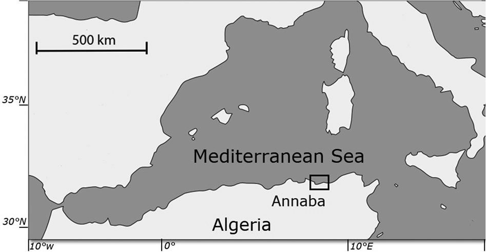
Fig. 1. Location of studied area in the south-western Mediterranean Sea.
To ensure a homogeneous distribution across all size classes, a subsample of 31 juvenile (220 < TL < 455) and 128 adult (455 < TL < 1210) individuals was taken from monthly samples for age determination (N = 159). Sagittal otolith pairs were extracted from each fish, cleaned and stored dry in Eppendorf tubes. Otolith length (OL), the longest distance between the frontal and hindmost points of the otolith, was measured in millimetres with a digital caliper (0.01 mm accuracy). One sagittae per fish was mounted and fixed on glass slides with a thermoplastic polymer (Crystal Bond). Otoliths were then sanded progressively finer (600–1000 mm) to obtain a fine cross-section passing through the nucleus. Polishing was performed with fine-grained sanding discs (3, 1 and 0.3 μm). The otoliths were then observed under a microscope. Age estimates were based on a count of both swift and slow growth, as already defined and described by Irie (Reference Irie1960), which resulted in alternating dark and illuminated light strips observed after thin transverse sections of sagittae. Growth rings were visible as alternating opaque and translucent zones, and ages were assigned to fish specimens based on their counts (one opaque zone combined with one translucent zone was interpreted as one year of growth). Counting was from the nucleus to the rostrum or post rostrum of otoliths because the latter grew much more along the antero-posterior axis. The width of each ring (OLi) and the length of each otolith radius were measured on this axis to the nearest 0.01 mm. A high-resolution microscope with an integrated camera (Visilog 5, Noésis) was used to obtain all measurements. Marginal increment analysis was used to validate annual growth increment formation (Beamish & McFarlane, Reference Beamish and McFarlane1983). The monthly mean marginal increment (MI) was calculated using MI = (R – Rn)/(Rn – Rn−1). R, Rn and Rn−1 are the radius, the radius of the last, and the radius of the next-to-last growth rings, respectively. Monthly values of MI were compared using a one-way ANOVA test, followed by a multiple-sample comparison of means (Dagnelie, Reference Dagnélie1975). Linear regression analysis was applied to evaluate the link between fish size (TL) and otolith radius size (RL). In accordance with the Fraser–Lee procedure (Carlander, Reference Carlander1981; Francis, Reference Francis1990), the length at age (TLi) was back-calculated as follows: TLi = a + (TLc – a) RLc −1 RLi, where a is the intercept of the TL–RL regression, TLc and RLc are the fish length and otolith radius size at capture, respectively, and RLi is the annulus width. The coefficient of determination (r 2) was used to evaluate the quality of the TL–RL regression.
Annular ring counts were made independently by two readers, who were blinded to information about fish length and date of capture. All otoliths were read twice, and final age estimates were achieved when the same results were obtained from the two readers. A third reading was performed if the first two readings differed from each other. If agreement could not be reached, the otolith was discarded. The average error index (APE) (Beamish & Fournier, Reference Beamish and Foumier1981) and the variation coefficient mean (CV) (Chang, Reference Chang1982) were used to compare the reading results. Observed lengths at different ages were compared with the back-calculated data by Student's t-test. The same test was used to compare growth between sexes. The von Bertalanffy growth function (von Bertalanffy, Reference Von Bertalanffy1938) was fitted to the length at age dataset back-calculated using FiSAT II software (Gayanilo et al., Reference Gayanilo, Sparre and Pauly2005). Von Bertalanffy growth parameters (L∞, k, t 0) were calculated by pooling ageing data of males and females. A likelihood-ratio test (Kimura, Reference Kimura1980) was calculated to test whether there were differences in growth between the sexes. The growth performance index Ø = 2 log L∞ + log k (Munro & Pauly, Reference Munro and Pauly1983) was calculated to compare the growth of this species with those of other Sphyraenidae. The relationship between length and weight was described by the power function EW = aTLb, where EW is the eviscerated weight. The regression parameters a and b and the coefficient of determination (r 2) were estimated for the whole population and for each sex by the least square linear regression after log transformation of both variables. According to Ricker (Reference Ricker1975), the slope of the regression was corrected to follow a geometric mean regression. Student's t-test was used to appreciate the hypothesis of isometric relationships, whereas analyses of covariance (ANCOVA) were used to detect any significant differences in the linear relationships between sexes (Zar, Reference Zar2010).
The total mortality rate (Z) was estimated using catch curve analysis, converted in length using the FiSAT II program (Gayanilo et al., Reference Gayanilo, Sparre and Pauly2005). Pauly's method (Pauly, Reference Pauly1980) and Ralston's regression method (Ralston, Reference Ralston, Polovina and Ralston1987) were applied to estimate the natural mortality rate (M). Fishing mortality (F) was assessed as follows: F = Z – M, and the exploitation rate was determined using the formula E = F/Z. Statistical analyses were performed with the MINITAB 18 software package.
Results
The Shapiro–Wilk normality test was W = 0.914, with P = 0.01, indicating that the sample came from a normal population distribution. Among the 698 sampled individuals, 169 were females (379–1210 mm TL, 192–7125 g), 102 were males (395–1165 mm TL, 226–5155 g) and 427 were immature (184–567 mm TL, 25–685 g) (Figure 2). The pooled length frequency distribution showed that younger fish (180–450 mm, < 1 year old) represented ~60% of the total catch. Applying the χ2 test for goodness of fit, the sex ratio was 1:1.65 in favour of females (χ2 = 16.56, df = 1, P > 0.1). The otolith length (OL) ranged from 4–24.3 mm. The relationship between the otolith radius OR (1.324 < OR mm < 3.922) and TL (401 < TL mm < 1210) was TL = 301.5 × RL – 82.4 (N = 137, r 2 = 0.856) (Figure 3). Comparisons of otolith age readings indicated good consistency or reproducibility (APE = 2.65%, CV = 3.75%). There was no statistically significant difference between readings (t = 1, df = 159, P > 0.05). Comparing successive monthly mean marginal increment (MI) values of otoliths using one-way ANOVA (F = 4.24, P < 0.0001) showed a significant difference between June and July (Figure 4).
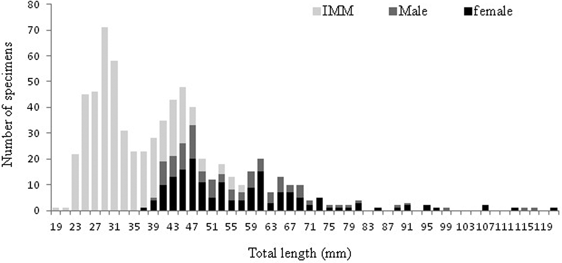
Fig. 2. Length frequency of males, females and immature individuals (IMM) of Sphyraena viridensis sampled in eastern coast of Algeria.
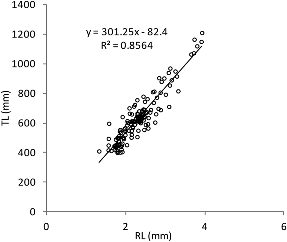
Fig. 3. Scatter plot and fitted regression line of fish length (TL) vs maximum radius size (RL) of Sphyraena viridensis in eastern coasts of Algeria.
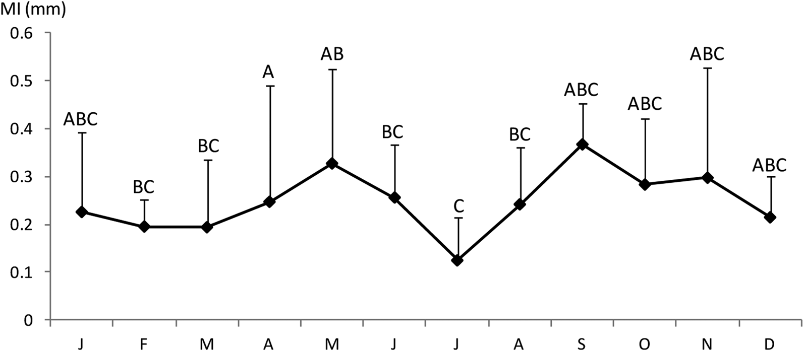
Fig. 4. Monthly evolution of otolith marginal increment of Sphyraena viridensis in eastern coasts of Algeria: the different letters indicate significant differences between groups of months; error bars, standard deviations.
Direct reading of otoliths (Figure 5) indicated maximum observed ages of 14 years in males and 13 years in females. Most individuals were aged between 1 and 5 years: 1 (23.27%), 2 (25.78%), 3 (6.29%), 4 (5.66%) and 5 (2.51%) (Table 1). From 6 years old, the number of individuals per age group was very low: 4 for age 6 (1 male 880 mm, 3 females: 807, 903 and 940 mm), 2 for age 7 (1 male 916 mm, 1 female 950 mm), 1 individual for age 8 (female, 905 mm), 1 individual for age 9 (female, 1073 mm), 1 individual for age 10 (female, 1120 mm), 2 individuals for age 11 (1 male 1150 mm, 1 female 1065 mm), 1 individual for age 13 (female, 1210 mm) and 1 individual for age 14 (male, 1165 mm). Then, the back-calculated method was applied to ages 1–6 in females and to ages 1–5 in males (Table 2). For both sexes, linear growth was very rapid during the first year (427 mm). The annual growth rate decreased gradually (121.7 mm at 2 years, 94.4 mm at 3 years). After the third year, the mean annual growth rate was 40.8 mm.
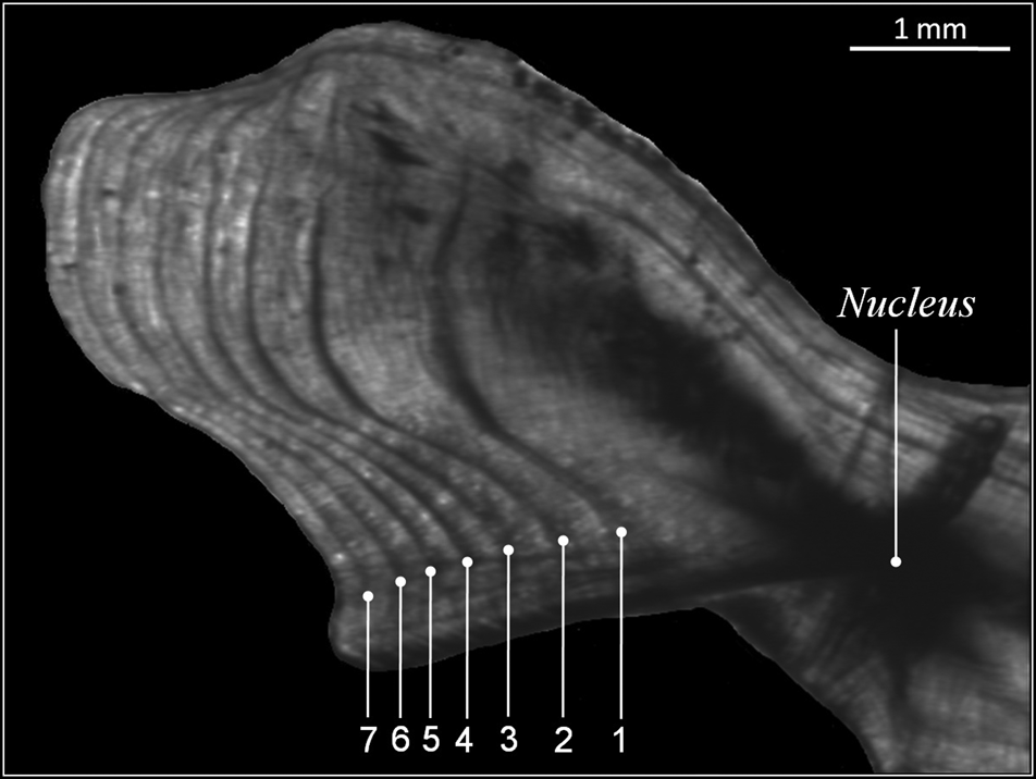
Fig. 5. Transverse section of sagittal otoliths of 7-year-old Sphyraena viridensis (751 mm TL) of the eastern coasts of Algeria. Numbers indicate annuli counted along the sulcal ridge.
Table 1. Age-length key of yellowmouth barracuda Sphyraena viridensis from eastern coasts of Algeria

N, number of fish; TL, mean length by age class; SD, standard deviation.
The numbers by sex of age groups 7 to 14 are low (< 3) and are indicated in the text (Materials and methods).
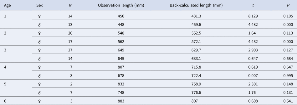
Table 2. Total length (mm) at the appearance of each growth ring in the sagittal section of the yellowmouth barracuda Sphyraena viridensis from eastern coasts of Algeria
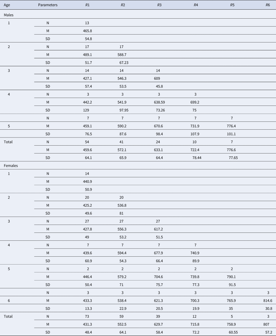
R1 to R6, growth rings in the sagittal section; N, number of fish; M, mean length by age class; SD, standard deviation.
The numbers by sex of age groups 7–14 are low (< 3) and are indicated in the text (Materials and methods).
The observed lengths at different ages did not vary significantly from the back-calculated lengths for males and females (Table 3). The back-calculated length at age did not significantly differ between sexes (unpaired t-test, all P > 0.05). Estimated von Bertalanffy growth models were TL = 1113 (1 – e −0.165(t+2.251)) (N = 58, 401 < TL mm < 1165) for males and TL = 958.3 (1 – e −0.247(t+1.422)) (N = 79, 402 < TL mm < 1210) for females. No significant difference was found between the male and female growth models (df = 3, P < 0.05); therefore, a combined-sex von Bertalanffy growth model of TL = 980.2 (1 – e −0.227(t + 1.655)) (N = 137, 402 < TL mm < 1210) was estimated (Figure 6). The predicted lengths at age using the combined-sex model were similar to the mean lengths at age back-calculated. The growth performance index (Ø) values were estimated to be 3.33 in both sexes, 3.44 in males and 3.35 in females.
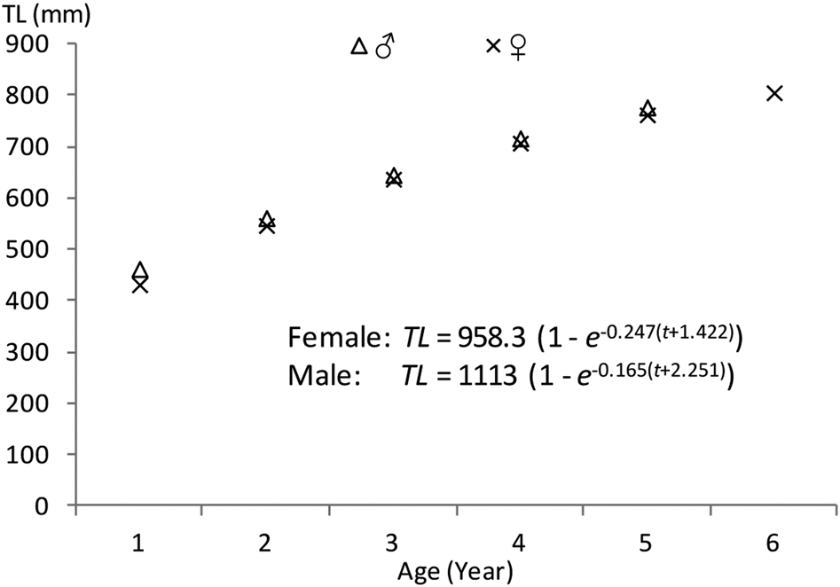
Fig. 6. Von Bertalanffy growth curves for Sphyraena viridensis in eastern coasts of Algeria.
Table 3. Comparison of observed and back-calculated lengths of Sphyraena viridensis from eastern coasts of Algeria

t, t-test; P = significance level; N, number of fish.
The numbers by sex of age groups 7 to 14 are low (< 3) and are indicated in the text (Materials and methods).
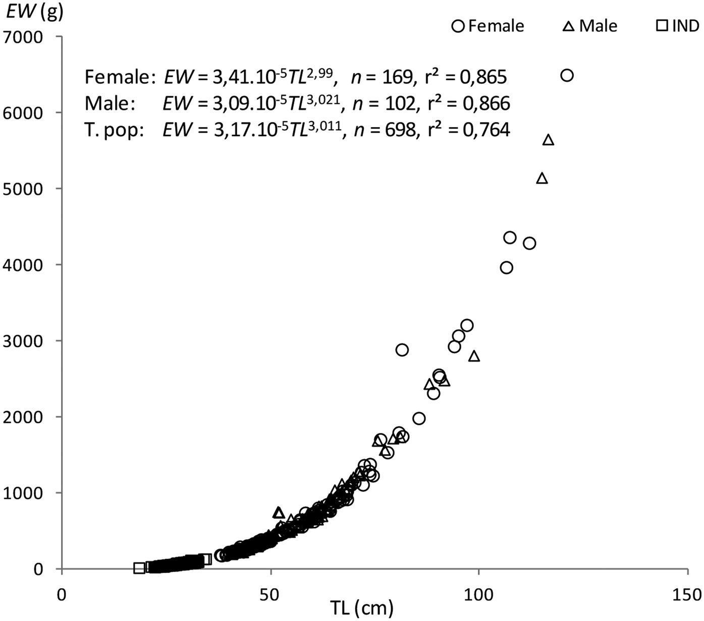
The length–weight relationships were EW = 3.09 × 10⁻⁵TL 3.021 (r2 = 0.866, N = 102, 395 < TL < 1165) in males, EW = 3.41 × 10⁻⁵TL 2.99 (r2 = 0.865, N = 169, 379 < TL < 1210) in females, and EW = 3.17 × 10⁻⁵TL 3.011 (r2 = 0.764, N = 698, 184 < TL < 1210) for both sexes combined. Significant differences were obtained from the comparison between males and females (ANCOVA, F = 56.18, P < 0.05). The b-values of the relationships indicate that the fish grew isometrically (t-test, t male = 0.19, t female = 0.103, P < 0.05) (Figure 7).

Fig. 7. Length-weight relationships of Sphyraena viridensis in eastern coasts of Algeria.
Using only fish fully recruited to the fishery (TL > 450 mm), we estimated total mortality Z = 0.51 year−1. Natural mortality estimate was M = 0.45 year−1. The estimate of fishing mortality (F) was 0.06 year−1, and the exploitation rate (E) was 0.11.
Discussion
This study is the first documented attempt to evaluate the age, growth and mortality of S. viridensis in the Western Mediterranean. The only available data on the population dynamics of this species in the Mediterranean are given by Allam et al. (Reference Allam, Faltas and Ragheb2004) in Egypt.
Sphyraena viridensis sagittal otoliths showed typical patterns of opaque and translucent alternating zones. The consistency, reproducibility and repeatability of the results (APE = 2.65%, CV = 3.75%) summarized and explained the reliability of the applied process. In agreement with Bourehail & Kara (Reference Bourehail and Kara2018), only one growth ring is formed per year during summer. This discontinuity in growth was observed by Kadison et al. (Reference Kadison, D'Alessandro, Davis and Hood2010) for S. barracuda from Florida Bay. This growth rhythm is described in a large number of fish species living in subpolar, temperate (Beckman & Wilson, Reference Beckman, Wilson, Secor, Dean and Campana1995) and tropical regions (Brothers, Reference Brothers1979).
Thirteen and fourteen age classes were determined by otolith readings in females and males, respectively. The oldest individual was a male of 1165 mm (14 years, 7125 g). Allam et al. (Reference Allam, Faltas and Ragheb2004) found a longevity of 8 years (560 mm TL) in Egyptian waters using otoliths. The longevities of Sphyraena sp. were 18 years for S. barracuda from Florida Bay (Kadison et al., Reference Kadison, D'Alessandro, Davis and Hood2010) and 11 years for S. argentena from California waters (Hart, Reference Hart1973).
The distribution of the ageing samples shows that the young-of-the-year (0+) fish were represented by fish less than 455 mm TL. More than 64% of the ageing samples were in age classes I–III. Ages V to VI were poorly represented (between 9 and 4 individuals by age). In Egyptian waters, Allam et al. (Reference Allam, Faltas and Ragheb2004) found that the individuals of age class II constituted the main bulk of catches (30%). In S. barracuda, an Atlantic Sphyraenidae with the same growth pattern, 50% of the fishes were aged between I and III years (Kadison et al., Reference Kadison, D'Alessandro, Davis and Hood2010).
During the first year of life, yellowmouth barracuda experienced rapid growth (over 50% of the maximal length observed in this study). Bourehail & Kara (Reference Bourehail and Kara2021) found similar rapid growth during the first year, while Allam et al. (Reference Allam, Faltas and Ragheb2004) found that S. viridensis from Egypt attained 26% of maximal length in the first year. The low growth rate after the first year of life may be related to the energetic costs of sexual maturation, which occurs at 625 and 595 mm in females and males, respectively (Bourehail et al., Reference Bourehail, Lecomte-Finiger and Kara2010), causing growth to slow down (Beverton & Holt, Reference Beverton and Holt1957).
Since this study represents the first separate estimations of male and female S. viridensis growth, it was not possible to compare them with other findings. The observed growth coefficient for pooled specimens (k = 0.227) is higher than that (k = 0.089) obtained by Allam et al. (Reference Allam, Faltas and Ragheb2004) in Egyptian Mediterranean waters. These differences could be due to the different hydrobiological conditions between the geographic areas. The estimated asymptotic length (L∞ = 980.2 mm) is similar to other estimates from the Mediterranean. The high r2 value of the combined-sex length-age von Bertalanffy growth model suggests that this curve accurately reflects somatic growth in these fishes (Figure 6). Of the growth parameters L∞ and k, only L∞ differed between the sexes (L∞ = 1113 mm in males, L∞ = 958.3 mm in females), indicating that the small difference between male and female curves was primarily a result of the greater longevity in males. Kadison et al. (Reference Kadison, D'Alessandro, Davis and Hood2010) also reported no significant difference between the growth models of males and females for S. barracuda from Florida Bay. The calculated growth performance index (3.33) is better than that in Egyptian Mediterranean waters (2.95) and among the higher indices in pelagic fish (Zischke & Griffiths, Reference Zischke and Griffiths2015). Values of the b coefficient in the length-weight relationship indicated isometric growth in females and males. In Egyptian waters, Allam et al. (Reference Allam, Faltas and Ragheb2004) found b = 2.93. Within the family Sphyraenidae, the type of growth is variable among species; for instance, negative allometric growth has been reported for S. ensis in Mexican waters (Zavala-Leal et al., Reference Zavala-Leal, Palacios-Salgado, Ruiz-Velazco, Valdez-González, Pacheco-Vega, Granados-Amores and Flores-Ortega2018) and for S. chrysotaenia from the Gulf of Gabes (Tunisia). In the Mediterranean Sea, Kalogirou et al. (Reference Kalogirou, Wennhage and Pihl2012) analysed the growth rates of S. viridensis (b = 2.76), S. sphyraena (b = 2.97) and S. chrysotaenia (b = 2.85) and found different types of growth even in species of the same region. For S. guachancho, different types of growth have been detected according to the sampling season (isometric growth in the rainy season and allometric growth in windy and dry seasons) (Bedia et al., Reference Bedia, Franco-López and Barrera-Escorcia2011). Begenal & Tesch (Reference Bagenal, Tesch and Bagenal1978) point out that differences in the length-weight relationship can be found with regard to sex, sexual maturity, season and even time of day as a result of stomach filling; therefore, changes in b value can be found in different developmental stages, at first sexual maturity and when important environmental changes occur.
The estimated average instantaneous rates of total (0.51 year−1), natural (0.45 year−1) and fishing (0.06 year−1) mortalities were lower than 2.8, 1.3 and 1.54 year−1, respectively, as recorded by Najmudeen et al. (Reference Najmudeen, Seetha and Zacharia2015) for S. obtusata of India.
The estimated fishing mortality indicates that S. viridensis is still facing a low exploitation rate in the Gulf of Annaba. Coupled with fisheries-independent surveys and commercial catch-at-age data, all the information provided here will contribute to improved fishery management of the Yellowmouth Barracuda S. viridensis in the south-western Mediterranean.
Acknowledgements
The authors thank the Algerian Ministry for Higher education and scientific research (General directorate for scientific research and technology development, GDRSDT) which financially supported this study, within the framework of the National Funds of Research (NFR).