


INTRODUCTION
Crassostreid oysters are protandric hermaphrodites (Kennedy, Reference Kennedy1983; Guo et al., Reference Guo, Hedgecock, Hershberger, Cooper and Allen1998). Guo et al. (Reference Guo, Hedgecock, Hershberger, Cooper and Allen1998) hypothesized that sex is determined by a two-allele system comprising a male dominant allele M and a protandric recessive allele F. Consequently, animals are of two genotypes: MF animals are permanent males (true males sensu Hoagland, Reference Hoagland1978; Guo et al., Reference Guo, Hedgecock, Hershberger, Cooper and Allen1998); FF animals are protandric animals. At old age, the expected sex-ratio is 3:1 female:male, given the anticipated equal likelihood of the two possible matings: FF × MF and FF × FF (Guo et al., Reference Guo, Hedgecock, Hershberger, Cooper and Allen1998). The cohort at sexual maturity, typically around a length of 35 mm and an age of ≤1 year (Burkenroad, Reference Burkenroad1931; Coe, Reference Coe1936; Hayes & Menzel, Reference Hayes and Menzel1981; O'Beirn et al., Reference O'Beirn, Heffernan, Walker and Jansen1996), is thought to be 100% functionally male. Observations show that sex-ratios in youngest mature Crassostrea virginica typically exceed 70% male (Dinamani, Reference Dinamani1974; Kennedy, Reference Kennedy1983; Paniagua-Chávez & Acosta-Ruiz, Reference Paniagua-Chávez and Acosta-Ruiz1995; Lango-Reynoso et al., Reference Lango-Reynoso, Chávez-Villaba and Pennec2006).
The presence of permanent males, originally proposed by Coe (Reference Coe1936), would seem a superfluity, as FF animals provide both functional males and functional females. However, sex- ratios may become highly skewed, all else being equal, in long-lived protandrous animals as the female phase likely has a much longer generation time than the male phase (Warner et al., Reference Warner, Robertson and Leigh1975; Gardner et al., Reference Gardner, Allsop, Charnov and West2005; Collin, Reference Collin2006). Other protandrous species have adaptations to stabilize the sex-ratio, including the alternation of protandry and protogyny in ostreids (e.g. Orton, Reference Orton1927, Reference Orton1936; Siddiqui & Ahmed, Reference Siddiqui and Ahmed2002), the influence of sedentary males in controlling the sex-ratio of Crepidula stacks (Coe, Reference Coe1938), and the lability of timing of the male-to-female switch (Charnov & Hannah, Reference Charnov and Hannah2002; see Buxton, Reference Buxton1993 for a protogynous example). In the same vein, Powell et al. (Reference Powell, Klinck and Hofmann2011a) argued that permanent males restrain the sex-ratio in adult crassostreids if long-lived. That is, a population composed solely of FF oysters, if long-lived, would tend to have a highly female-biased sex-ratio at carrying capacity when mostly older adult animals represent the population, and this bias would limit population reproductive capacity. Permanent males theoretically limit the sex-ratio to no higher than 3:1 in the same circumstance.
The eastern oyster Crassostrea virginica lives over a wide range of salinities characterized by a range of natural mortalities and hence life spans, and by a range of growth rates. Typically, natural mortality rises at higher salinity (e.g. Gunter, Reference Gunter1979; Haskin & Ford, Reference Haskin and Ford1982; Soniat & Brody, Reference Soniat and Brody1988; Dekshenieks et al., Reference Dekshenieks, Hofmann, Klinck and Powell2000), as does growth rate (e.g. Paynter & Burreson, Reference Paynter and Burreson1991; Kraeuter et al., Reference Kraeuter, Ford and Canzonier2003, Reference Kraeuter, Ford and Cummings2007). Over geological time, most of the salinity-dependent variation in natural mortality differentially affected the survivorship of new recruits, as many important predators focusing on juveniles increase in abundance down estuary (e.g. Engle, Reference Engle1953; Carriker, Reference Carriker1955; Provenzano, Reference Provenzano1961; Newell et al., Reference Newell, Alspach, Kennedy and Jacobs2000). The natural mortality rate of the adult contingent likely remained near 10% per year over much of the salinity range (Powell et al., Reference Powell, Ashton-Alcox, Kraeuter, Ford and Bushek2008), at least in north-eastern bays such as Delaware Bay, and life span likely reached 10–20 years. (Galtsoff (Reference Galtsoff1964) maintained C. virginica for at least 9 years, so Crassostrea likely can live for a decade or longer, considerably beyond the conservative estimates provided by Comfort (Reference Comfort1957) and Custer & Doms (Reference Custer and Doms1990), but consistent with estimates for fossil species (Kirby, Reference Kirby2000) and recent estimates reported in Berrigan et al. (Reference Berrigan, Candies, Cirino, Dugas, Dyer, Gray, Herrington, Keithly, Leard, Nelson and van Hoose1991); but see Harding et al. (Reference Harding, Mann and Southworth2008).) However, the onset of two diseases, MSX, caused by the haplosporidian Haplosporidium nelsoni, and Dermo, caused by the apicomplexan Perkinsus marinus, has reduced adult life spans significantly and in a salinity-dependent manner (Powell et al., Reference Powell, Klinck and Hofmann1996; Paraso et al., Reference Paraso, Ford, Powell, Hofmann and Klinck1999; Ragone Calvo et al., Reference Ragone Calvo, Wetzel and Burreson2001; Harding et al., Reference Harding, Mann and Southworth2008; see also Vølstad et al., Reference Vølstad, Dew and Tarnowski2008). Arguably, this voids the raison d'être for the MF animal, because adult mortality limits the number of females and thus regulates the sex-ratio (Powell et al., 2011a).
One consequence, however, of an expanded range of mortality rates of females along the estuarine salinity gradient may be a divergence in the sex-ratio between local populations. In reviewing the literature on C. virginica, Kennedy (Reference Kennedy1983) found sex-ratios consistent with subsequent expectations expressed by Guo et al. (Reference Guo, Hedgecock, Hershberger, Cooper and Allen1998). Kennedy (Reference Kennedy1983) also found that most sites examined retained population sex-ratios near 1:1 female:male despite the complications of protandry and that sex-ratio had changed little at most sites when compared over a decade or more despite likely variations in mortality and recruitment rates (e.g. Kennedy & Krantz, Reference Kennedy and Krantz1982). Kennedy (Reference Kennedy1983) stressed from a summary of observations by Burkenroad (Reference Burkenroad1931) and others, along with his own, that an increased proportion of functional males was associated with higher population density, suggesting that some compensatory process exists within populations controlling the sex-ratio besides the presence of permanent males. Finally, Kennedy (Reference Kennedy1983) proffered that increased environmental stress resulted in sex-ratios biased towards an increased proportion of functional males, in part due to the reversion of females to the male phase.
The oyster fishery selectively harvests animals ≥2.5″ (63.5 mm) in Delaware Bay (Powell et al., Reference Powell, Gendek and Ashton-Alcox2005) and ≥3″ (76 mm) in many other regions (e.g. Berrigan et al., Reference Berrigan, Candies, Cirino, Dugas, Dyer, Gray, Herrington, Keithly, Leard, Nelson and van Hoose1991). Thus, the fishery likely is biased in favour of females (Rothschild et al., Reference Rothschild, Ault, Goulletquer and Héral1994). Sex-biased fisheries are susceptible to overfishing (e.g. Sissenwine & Shepard, Reference Sissenwine and Shepherd1987; Rothschild et al., Reference Rothschild, Ault, Goulletquer and Héral1994; Rago et al., Reference Rago, Sosebee, Brodziak, Murawski and Anderson1998), as selective removal of females is much more likely to impact population reproductive capacity than the loss of males. The Delaware Bay fishery is managed under a strict quota system designed to encourage population sustainability (Klinck et al., Reference Klinck, Powell, Kraeuter, Ford and Ashton-Alcox2001; Powell et al., Reference Powell, Klinck, Ashton-Alcox and Kraeuter2009a); however, the biological reference points used to set quotas based on fishery-independent stock surveys and monitoring of landings are not influenced by the sex-ratio, as these data have not been available (Powell et al., Reference Powell, Klinck, Ashton-Alcox and Kraeuter2009b). Since 2000, recruitment rate has declined in Delaware Bay (HSRL, 2009) and one result has been the development of a population size frequency weighted towards the larger and older adult animals; presumably up to 75% of these animals may be female. Accordingly, closer attention to population sex-ratio during a time of restricted recruitment would be warranted.
The purpose of this study was to evaluate the sex-ratio in a C. virginica population over a wide salinity range to determine: (a) the degree to which salinity-dependent growth and mortality might be influencing sex-ratios in animals in which adult mortality is primarily controlled by Dermo disease; and (b) the sex-ratio of landings for application in the stock assessment process. To do this, we sampled all major oyster populations in the New Jersey waters of Delaware Bay, using a protocol that would permit reconstitution of the local population's sex-ratio based on sex-at-length keys developed by the sampling programme and size–frequency data obtained by survey.
MATERIALS AND METHODS
Four sampling locations were chosen on each of 18 of the natural oyster beds in the New Jersey waters of Delaware Bay (Figure 1). In addition, three sites were taken from the most up estuary bed, Hope Creek, and one from a neighbouring bed, Liston Range. Samples were also taken from three peripheral sites: one sample from each of two river sites, Cohansey and Maurice, and one sample from a down estuary site, the Cape Shore flats (Figure 1). The Cape Shore flats are an area where high recruitment occurs routinely (Nelson, Reference Nelson1959), but adult oysters do not occur there in marketable abundance due to extremely high juvenile mortality. The two river sites and the Hope Creek/Liston Range site represent the low-salinity extremes of the population's range.

Fig. 1. The location of sampling sites on the footprint of the Delaware Bay natural oyster beds in New Jersey waters delineating also the high-quality (dark shade) from the medium-quality (light shade) grids. Each bed is defined in terms of a set of rectangular grids 0.2′ latitude × 0.2′ longitude in size, equivalent to approximately 25 acres. These grids also serve as survey sampling units (Powell et al., Reference Powell, Ashton-Alcox, Kraeuter, Ford and Bushek2008). Ledge and Egg Island beds have not been re-surveyed. For the remaining beds, the depicted footprint is based on re-surveys that occurred in 2005–2008 (Powell et al., Reference Powell, Klinck, Ashton-Alcox and Kraeuter2009a).
The Delaware Bay stock assessment survey uses a stratified random sampling protocol. Strata differentiate high, medium, and low-quality areas on each bed based on relative oyster abundance (HSRL, 2009). Samples were taken from the high and medium-quality strata only; normally two samples came from each stratum on each bed. Sampling occurred over the course of four days from 17 June to 3 July 2008. At each site, one or more dredge hauls were taken, sufficient to provide at least one bushel (37 l) of material and 100 animals for measurement. In some cases, multiple hauls and multiple bushels were required to reach the 100-animal goal.
The length (anterior–posterior) of all animals ≥20 mm in the bushel haul was measured. Animals were assigned to a sequence of 10-mm bins from each of which were chosen haphazardly ten animals, or all animals were taken if fewer than ten, for sex determination. The four sampled sites from each bed thus yielded up to 40 sexed animals total for each 10-mm bin for each bed. This subsampling design assured that a representative number of animals were chosen to adequately define the local population size frequency for males and females on each bed. Routinely the largest bin was not fully filled; a plus group was thus established for subsequent analysis such that minimally 10 animals were assigned to this largest size-class. Sex was determined by shucking each oyster, poking the gonadal tissue with a capillary tube, expelling the contents onto a microscope slide, adding a drop of seawater and a cover slip, and examining the slide microscopically. Animals were identified as male (sperm present), female (eggs present), simultaneous hermaphrodites (eggs and sperm present), or undifferentiated (no gametes present).
Bed-level and larger-scale population sex-ratios were obtained by formulating a sex-at-length key for each bed. Population sex-ratios were developed using the 100+ length measurements from all four samples per bed plus the sex-at-length key; thus, no effort was made to distinguish samples from high-quality and medium-quality areas in data analysis. Length-based data were converted to weight-based units using autumn 2007 and autumn 2008 length–weight relationships developed separately for each bed (HSRL, 2008, 2009).
Statistical analyses were of three types. Binomial tests followed Conover (Reference Conover1980). Frequency distributions were compared using two-sample two-sided Kolmogorov–Smirnov (K-S) tests (Conover, Reference Conover1980). Parameters of model equations were compared using randomization tests (Noreen, Reference Noreen1989). Most ratio comparisons were analysed using binomial statistics. An issue arises as to the proper n or number of occurrences to use in these analyses as many more individuals were measured to establish the population size frequency than were sexed in nearly all cases. To retain the statistical evaluation at the level of the original dataset, reconstructed population sex-ratios were proportionately reduced to a total number of individuals equivalent to the number sexed. This standardization corrected each data subset to the minimal n supporting the original sex-at-length key and generated, therefore, a conservative test statistic.
The relationship of fraction female with length, L, or age was modelled as a Gompertz curve:
 $$Fraction \ female = \alpha_{l} e^{\beta_{l} e^{\gamma_l \, L\lpar mm\rpar }}\eqno\lpar 1\rpar$$
or
 $$Fraction \ female = \alpha_{a} e^{\beta_{a} e^{\gamma _{a}\, age\lpar yr\rpar }}.\eqno\lpar 2\rpar$$
The Gompertz curves were compared using randomization tests. In each case, 1000 subsets of individuals were chosen with replacement from the individuals representing the remainder of the dataset, excluding the region of interest. The number in each subset was determined by the number of original observations in the region of interest. The parameters for the observed Gompertz curve were then compared individually with the parameters from the 1000 subsamples to evaluate the likelihood of their occurrence in a random subset of the remainder of the data once the region of interest was excluded. In addition, the sum of the normalized residuals was calculated for each subset as
 $$Sum \ of \ the \ residuals = \sum\nolimits_{i=1}^n \left({\textstyle{{\; observed\; fraction - expected\; fraction} \over {median\; size\; class\; length}}}\right)\eqno\lpar 3\rpar$$
where n is the number of 10-mm increments used for the Gompertz curve fit, expected is the fraction female derived from the Gompertz fit for the random subsample, and observed is the fraction female derived from the Gompertz fit for the region of interest. The distribution of the sign of the sums was evaluated relative to an expected 50:50 split using a binomial test.
RESULTS
Descriptive statistics
Most oyster beds yielded a sufficient number of animals covering a range of sizes to provide 20 or more animals to be sexed per 10-mm size-class from 20 mm to 100+ mm (Table 1). The most down bay beds, Egg Island and Ledge, yielded animals restricted to a few of the larger size-classes. This is consistent with the condition of these beds over many years in which abundances have been low and recruitment sporadic. The river sites also yielded relatively few animals in the smaller size-classes. The most up bay sites provided few of the largest animals; particularly depauperate were animals >100 mm in size. This also is consistent with long-term trends. Growth rates routinely are slowest and maximum sizes smallest on these beds (Kraeuter et al., Reference Kraeuter, Ford and Cummings2007).
Table 1. The number of individuals sexed for each oyster bed, reported in 10-mm increments. Bed locations are shown in Figure 1. Headers are the medians for each 10-mm size-class except for the plus group (last column) that is ≥100 mm.

The fraction of the animals sexed that were female, disregarding the few simultaneous hermaphrodites found for each 10-mm size-class, is provided in Table 2. Each site shows the anticipated trend of increasing fraction female with increasing size. For simplicity, in further analyses, beds are coalesced into regions established by gradients in natural mortality (and hence life span) and growth (and hence maximum size) that are well-established regional conglomerates routinely used for the assessment of the Delaware Bay stock (Haskin & Ford, Reference Haskin and Ford1982; Kraeuter et al., Reference Kraeuter, Ford and Cummings2007; Powell et al., Reference Powell, Ashton-Alcox, Kraeuter, Ford and Bushek2008, Reference Powell, Klinck, Ashton-Alcox and Kraeuter2009a) (Figure 2). Not included in these groupings are the two river sites, henceforth combined, and the Cape Shore flats that are retained discrete.

Fig. 2. The location of sampling sites in the bed regions established based on long-term trends in growth and mortality (Powell et al., Reference Powell, Ashton-Alcox, Kraeuter, Ford and Bushek2008).
Table 2. The fraction female
 ${\big({F \over {F+M}}\big)}$
for each oyster bed. The location of each bed is provided in Figure 1. –, no data. Headers are the medians for each 10-mm size-class except for the plus group (last column) that is ≥100 mm.
${\big({F \over {F+M}}\big)}$
for each oyster bed. The location of each bed is provided in Figure 1. –, no data. Headers are the medians for each 10-mm size-class except for the plus group (last column) that is ≥100 mm.

Most oysters could be sexed, regardless of region (Table 3). Oysters of indeterminate sex were rare above 40 mm and only relatively common at <30 mm. This is consistent with observations of size at maturity as previously referenced. Even for the smallest size-class (20–30 mm), the number of indeterminate sex did not exceed 16% except in one case, the very-low-mortality beds. With this exception, an influence of the salinity gradient was not apparent. Oysters of unassigned sex may bias sex-ratios. With the exception of the smallest size-class, little bias exists in this dataset, and these oysters are ignored in further analyses.
Table 3. The fraction of sexed animals that were of indeterminate sex, by bay region. Headers are the medians for each 10-mm size-class except for the plus group (last column) that is ≥100 mm. Bay regions are shown in Figure 2 and defined in Table 1. –, no data.

Simultaneous hermaphrodites were also infrequent (Table 4), rarely exceeding 3% of the animals in any 10-mm size-class. Incidences above 4% were noted only in animals <40 mm, with highest occurrence rates tending to be found up estuary of the high-mortality beds. Simultaneous hermaphrodites henceforth are not included in the calculation of any sex-ratio.
Table 4. The fraction of sexed animals that were simultaneous hermaphrodites, by bay region. Headers are the medians for each 10-mm size-class except for the plus group (last column) that is ≥100 mm. Bay regions are shown in Figure 2. –, no data. Beds coalesced into each region are identified in Table 1.

The fraction female rose from values on the order of 10% in the 20-to-30-mm size-class to values on the order of 75% for the ≥100-mm group (Table 5). The fraction female in the larger size-classes was distinctly lower for the river sites and for the very-low-mortality beds and distinctly higher for the Cape Shore flats. However, the distribution of sex-ratios across the size–frequency spectrum was not significantly different for any pairwise comparison between regions (K-S test, α = 0.05), except one, when the analyses were restricted to a plus group with adequate sample size (e.g. >10 individuals). The exception was the comparison of the high-mortality and medium-mortality beds (P < 0.05). However, the application of the K-S test is restricted by the great likelihood that the sex-ratios of the smaller size-classes will be similar because all or nearly all animals mature initially as males; thus, divergence in the sex-ratio with size between datasets should manifest itself predominately in the few highest size-classes, if at all. For this reason, in a later section, we use randomization tests to compare trends in sex-at-length between bay regions.
Table 5. The fraction of sexed animals that were female
 ${\big(\textstyle{F \over {F+M}}\big)}$
, by bay region. Headers are the medians for each 10-mm size-class except for the plus group that represents animals ≥100 mm. For two regions, for which a sufficient number of larger animals is available, three additional groups are also provided, including a plus group ≥120 mm. Bay regions are shown in Figure 2. –, no data; NA, insufficient data. Beds coalesced into each region are identified in Table 1.
${\big(\textstyle{F \over {F+M}}\big)}$
, by bay region. Headers are the medians for each 10-mm size-class except for the plus group that represents animals ≥100 mm. For two regions, for which a sufficient number of larger animals is available, three additional groups are also provided, including a plus group ≥120 mm. Bay regions are shown in Figure 2. –, no data; NA, insufficient data. Beds coalesced into each region are identified in Table 1.

We asked whether the sex-ratio for each of the size-classes and bay regions differed significantly from 1:1 male:female (Table 6). We could not differentiate permanent from protandric males for these tests; thus animals were allocated by functional sex. Most ratios for animals 20–50 mm diverged significantly from 1:1, regardless of bay region. These size-classes were enriched in males. Most size-classes ≥80 mm also diverged significantly from 1:1. These size-classes were enriched in females. The river sites were noteworthy in departing from this trend. In this case, the higher size categories remained indistinguishable from a 1:1 ratio. In most cases animals 60–80 mm had sex-ratios near 1:1.
Table 6. Results of binomial tests to determine whether each of the sex-ratios reported in Table 5 diverges from a 1:1 female:male ratio. Headers are the medians for each 10-mm size-class except for the plus group (last column) that is ≥100 mm. –, no data; NA, insufficient data; *********, significant at α = 0.0001; ********, significant at α = 0.0005; *******, significant at α = 0.001; ******, significant at α = 0.005; *****, significant at α = 0.01; ****, significant at α = 0.02; ***, significant at α = 0.025; **, significant at α = 0.05; *, significant at α = 0.10; blank, not significant at α = 0.10.

The sex-ratios of even the smallest size-class examined (20–30 mm) diverged significantly from the expectation of 0% female (Table 7). At the other extreme, most sex-ratios for the largest size-classes did not diverge significantly from the expected 3:1 female:male ratio (Table 8). Of those that did for animals ≥90 mm, the result was obtained by a superfluity of males, except in one case. The sex-ratio for animals 110–120 mm on the high-mortality beds was significantly biased in favour of females, relative to the 3:1 expectation.
Table 7. Results of binomial tests to determine whether each of the sex-ratios reported in Table 5 diverges from 0% female, the all-male condition. Headers are the medians for each 10-mm size-class except for the plus group (last column) that is ≥100 mm. –, no data; NA, insufficient data; blank, not significant at α = 0.10; *********, significant at α = 0.0001.

Table 8. Results of binomial tests to determine whether each of the sex-ratios reported in Table 5 diverged from 3:1, the 75% female condition anticipated if 25% of the older individuals are permanent males. For the high-mortality and medium-mortality regions, for which a sufficient number of larger animals are available, three additional groups are also provided. Headers are the medians for each 10-mm size-class except for the plus groups that are ≥100 mm and ≥120 mm, respectively. –, no data; NA, insufficient data; *********, significant at α = 0.0001; ********, significant at α = 0.0005; *******, significant at α = 0.001; ******, significant at α = 0.005; *****, significant at α = 0.01; ****, significant at α = 0.02; ***, significant at α = 0.025; **, significant at α = 0.05; *, significant at α = 0.10; blank, not significant at α = 0.10.

Population sex-ratios
A sex-at-length key was applied to each of the bed size–frequency distributions and the resulting numbers of females and males used to construct a sex-ratio for each region (Figure 2) and the population as a whole. Analyses were conducted in two ways. First, analyses were based solely on the size–frequency distributions obtained in the June–July 2008 samples. These analyses do not take into account variations in abundance between beds coalesced into bay regions. However, they do permit comparison to the Cape Shore flats and river sites. As an alternative, we used the October 2007 and October 2008 stock assessment data (HSRL 2008, 2009). This permits accurate weighting of the population and regional sex-ratios by bed abundance; however, perforce, the river sites and the Cape Shore flats site were deleted, as these sites are not included in the yearly stock survey (Powell et al., Reference Powell, Ashton-Alcox, Kraeuter, Ford and Bushek2008).
The summer 2008 collections supplying the sex-at-length keys combined with the size–frequency of the oysters simultaneously obtained show population female fractions varying from 0.41 to 0.52 (Figure 3). With one exception, the populations in all bay regions are moderately biased in favour of males. In only two cases are the sex-ratios significantly divergent from a 1:1 female:male ratio (α = 0.05). We also utilized the 2007 and 2008 survey data. All female fractions fell below 0.5 with one exception (Figure 4), most varying between 0.41 and 0.47. In 2007, two of five bay regions diverged significantly from a 1:1 female:male ratio. In 2008, all did (Figure 4). In both years, the low-mortality beds had a higher proportion of females, with lower proportions both up estuary and down estuary from this region.

Fig. 3. The fraction female in June–July 2008, in Delaware Bay, based on a series of collections from the oyster beds identified in Table 1. The ratios are corrected for the size frequency upon collection for each individual bed and the bed sample values summed to provide regional estimates, uncorrected for variations in total abundance between beds. Statistics are P values obtained from binomial tests with an expected fraction of 0.5 (a 1:1 female:male ratio). Blank, not significant at α = 0.10.
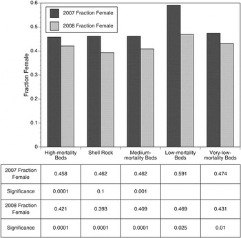
Fig. 4. The fraction female in Delaware Bay estimated from the 2007 and 2008 stock surveys, based on summer 2008 sex-at-length keys and the survey values obtained in October of the respective years. The ratios are corrected for the size frequency obtained by the survey for each individual bed and the bed values summed to provide regional estimates. Bed values summed are weighted by the total abundance of each bed. Statistics are P values obtained from binomial tests with an expected fraction of 0.5 (a female:male ratio of 1:1). Blank, not significant at α = 0.10.
Converting the 2007 and 2008 survey data to biomass reveals that females routinely contribute 65–75% of the biomass in each bay region. No obvious trends exist with the salinity gradient (Figure 5).

Fig. 5. Comparison of the fraction female in Delaware Bay based on biomass and abundance estimated for the 2007 and 2008 stock surveys, using summer 2008 sex-at-length keys, bed-specific length-to-weight conversions from the 2007 survey, and the survey values obtained in October of the respective years. The ratios are corrected for the size frequency obtained by the survey for each individual bed and the bed values summed to provide regional estimates. Bed values summed are weighted by the total abundance or biomass of each bed.
Trend in sex-ratio with length and age
The trend of sex-ratio with length and age followed a Gompertz curve for each of the seven regional groups (Figure 6) with parameter values listed in Table 9. The Gompertz relationship is commonly used to model growth (McCuaig & Green, Reference McCuaig and Green1983; Devillers et al., Reference Devillers, Eversole and Isely1998; Ohnishi & Akamine, Reference Ohnishi and Akamine2006). Four of the curves in Figure 6 nearly overlay each other and these regions account for about 75% of the total New Jersey population in Delaware Bay: namely the high-mortality beds, Shell Rock, the medium-mortality beds, and the low-mortality beds (Figure 2). Three are outliers in some sense. Overall, the range extremes all constitute outlier populations. The Cape Shore flats population manifests a higher rate of male conversion to female with increasing length. The river sites exhibit a distinctly opposing trend. The very-low-mortality beds display a more average conversion rate over the smaller size-classes, but conversion appears to cease prematurely, yielding an unusually small fraction female in the larger size-classes (Figure 6). Arguably, from Guo et al. (Reference Guo, Hedgecock, Hershberger, Cooper and Allen1998), 25% of the males are permanent males and, thus, cannot convert to females. Examples for two of the same plots corrected thus are compared to the originals in Figure 7. Trends and parameter values are identical except that the αl modified from equation (1) is:
 $\alpha_{\rm mod}={\textstyle{{\alpha_l} \over {0.75}}}$
.
$\alpha_{\rm mod}={\textstyle{{\alpha_l} \over {0.75}}}$
.


Fig. 7. Examples of two curves from Figure 6 comparing the relationship of the fraction female versus length for the entire population and for the putative protandric component only, based on the assumption that 25% of the animals are permanent males.
Table 9. Parameters of Gompertz curve fits for the seven bed regions for the relationship between fraction female and length or age. The equation is
 $Fraction\; female=\alpha_{l \, } e^{\beta_{l \, } e^{\gamma_l \, L\lpar mm\rpar }}$
or
$Fraction\; female=\alpha_{l \, } e^{\beta_{l \, } e^{\gamma_l \, L\lpar mm\rpar }}$
or
 $Fraction\; female=\alpha_{a \, } e^{\beta_{a \, } e^{\gamma _{a\,} age\lpar yr\rpar }}$
.
$Fraction\; female=\alpha_{a \, } e^{\beta_{a \, } e^{\gamma _{a\,} age\lpar yr\rpar }}$
.

Randomization tests comparing the curves shown in Figure 6 confirm the unusual nature of the relationship of sex-ratio and size in oysters from the very-low-mortality beds (Table 10). None of the three Gompertz parameters for this region (Table 9) are likely to occur by chance from subsets of oysters collected elsewhere (Table 10). The curve is altogether different in form. The low-mortality beds are less aberrant; however, the βl value significantly diverges from that expected from chance subsets of oysters from the remaining regions and the remaining two parameters would do likewise at α = 0.10. In addition, the curve, overall, shows significantly higher fractions female at size, indicating that the male-to-female conversion occurs more rapidly at smaller size in this region than for the population as a whole. Note that the same tendency, though more extreme, exists for the intermediate size-classes for oysters from the very-low-mortality beds, but in this case the outcome at largest size is truncated so that the largest animals remain over-represented by males. This leads to the significantly different form of the Gompertz relationship for animals collected from this region.
Table 10. Uniqueness of the parameters of Gompertz fits for the seven bed regions for the relationship between fraction female and length or age, based on randomization tests. The equation is
 $Fraction\; female=\alpha_{l \, } e^{\beta_{l \, } e^{\gamma_l \, L\lpar mm\rpar }}$
or
$Fraction\; female=\alpha_{l \, } e^{\beta_{l \, } e^{\gamma_l \, L\lpar mm\rpar }}$
or
 $Fraction\; female=\alpha_{a \, } e^{\beta_{a \, } e^{\gamma _{a\,} age\lpar yr\rpar }}$
. P values are obtained by independently ranking 1000 estimates of each parameter obtained from 1000 subsets of the data remaining after exclusion of the region of interest. Also provided is the proportion of the subsets yielding negative sums of the normalized residuals obtained by comparison of the observed female fractions calculated from the Gompertz curve (Table 9) with the equivalent values from a Gompertz curve obtained by random selection of the same number of individuals from the remaining data set (Equation (3)). For the three Gompertz parameters, significant differences occur with P ≤ 0.05 or P ≥ 0.95. For the residuals, the likelihood that the observed number of negative values was obtained by chance is also provided.
$Fraction\; female=\alpha_{a \, } e^{\beta_{a \, } e^{\gamma _{a\,} age\lpar yr\rpar }}$
. P values are obtained by independently ranking 1000 estimates of each parameter obtained from 1000 subsets of the data remaining after exclusion of the region of interest. Also provided is the proportion of the subsets yielding negative sums of the normalized residuals obtained by comparison of the observed female fractions calculated from the Gompertz curve (Table 9) with the equivalent values from a Gompertz curve obtained by random selection of the same number of individuals from the remaining data set (Equation (3)). For the three Gompertz parameters, significant differences occur with P ≤ 0.05 or P ≥ 0.95. For the residuals, the likelihood that the observed number of negative values was obtained by chance is also provided.

The other two outlier locations, the river sites and the Cape Shore flats, do not demonstrate unusual Gompertz parameters (Table 10), nor does Shell Rock. The medium-mortality beds, however, are described by Gompertz parameters that are unlikely to have come from the remaining population by chance, as is also the case for the high-mortality beds (Table 10). A pairwise comparison between the high-mortality and medium-mortality beds and the low-mortality and medium-mortality beds confirms the uniqueness of the medium-mortality beds. Most Gompertz parameters describing the relationship between fraction female and length for the medium-mortality beds are unlikely to have been obtained by chance sub-samplings of the animals from either of the other two bed regions (Table 10).
The sums of the residuals obtained by comparison of any one bed region with random subsets taken from the remaining regions demonstrate that the river beds, the medium-mortality beds, and the high-mortality beds show fractions female at size significantly below the remaining beds. A pairwise comparison of the high-mortality and medium-mortality beds shows that the random subsets from one provide overall higher or lower fractions female at size than the other relatively frequently; these curves cross rather than running sub-parallel above or below each other, hence the significantly different Gompertz parameters. A pairwise comparison between the low-mortality and medium-mortality beds is consistent with the significantly higher (less negative) βl and γl parameters for the low-mortality beds (Table 9) in that the rate of male-to-female conversion with length is routinely higher. That is, a negative residual sum occurs in every comparison between the observed medium-mortality trend and the 1000 random subsets taken from the low-mortality dataset.
The rate of conversion from male to female can be evaluated with age, rather than length, for four bay regions for which von Bertalanffy equations were reported by Kraeuter et al. (Reference Kraeuter, Ford and Cummings2007) (Figure 8). For three of the four regions, the rates of male-to-female conversion relative to oyster age are similar: the high-mortality beds, Shell Rock, and the medium-mortality beds. For the low-mortality beds, the rate of conversion is decidedly slower, although the asymptotic fraction female is about the same at oldest age.

Fig. 8. The relationship of fraction female with age for four bay regions for which estimates can be made. Age was estimated from length using the von Bertalanffy relationships of Kraeuter et al. (Reference Kraeuter, Ford and Cummings2007). Curves are best-fit Gompertz curves. Gompertz-curve parameterizations are given in Table 9.
Randomization tests confirm the uniqueness of the low-mortality beds (γa value: Tables 9 & 10), but also the high-mortality beds (αa value). The distinctiveness of the low-mortality curve is reaffirmed by pairwise comparison with the medium-mortality beds. The sums of the residuals are routinely positive: the medium-mortality curve falls above the low-mortality curve, indicating a more rapid male-to-female conversion with age. The converse trend exists in the pairwise comparison between the medium-mortality and high-mortality beds.
DISCUSSION
The genetic basis for sex determination
Guo et al. (Reference Guo, Hedgecock, Hershberger, Cooper and Allen1998) forwarded the hypothesis that sex in crassostreid oysters is determined by a two allele system, a dominant male allele and a recessive protandric allele. Thus, oysters would be either MF permanent males or FF protandric individuals. Two expectations ineluctably issue from this hypothesis. First, all young animals should be functionally male. Second, older adults should be 75% female.
A review of the literature shows that females rarely occur among the youngest mature oysters (Dinamani, Reference Dinamani1974; Kennedy, Reference Kennedy1983; Paniagua-Chávez & Acosta-Ruiz, 1995; Lango-Reynoso et al., Reference Lango-Reynoso, Chávez-Villaba and Pennec2006). In our dataset, the proportion of females 20-to-30 mm in size rarely exceeded 20% on any bed. The value for the entire dataset was 13.9%. Values below 15% occurred in 15 of 23 locations sampled. Cases in which males exclusively were observed occurred in 7 of 23 locations. In four of these cases, the number of observations was small (Table 1) and the resulting collection of males only could have occurred by chance (α = 0.05). For the other three, however, the absence of small females by chance is unlikely (Hope Creek, P = 0.00088; Round Island, P = 0.01; Upper Middle, P = 0.006). The strong inference follows that most oysters are indeed initially functionally male. When the various beds were combined into regions, in 6 of 7 cases, the sex-ratio of animals in the 20-to-30-mm size-class diverged significantly from the expectation of 0% female (Table 7). So, although uncommon, small functional females occurred routinely throughout the environmental range sampled in Delaware Bay. The 20-to-30-mm animals were very likely nearly one year old (Kraeuter et al., Reference Kraeuter, Ford and Cummings2007), and almost certainly collected prior to their first spawn. Thus, it seems likely that some protandric animals, even if initially male, convert to female so early in life that they never perform as functional males.
An alternative to the Guo et al. (Reference Guo, Hedgecock, Hershberger, Cooper and Allen1998) hypothesis would entail a system of sex determination that includes permanent females. One such alternative consists of a MM permanent male, a FF permanent female, and a MF protandric animal (Powell et al., Reference Powell, Klinck and Hofmann2011a). However, under this system, all sites should contain some small functional females, whereas we observed exclusively males at 7 of 23 locations. Powell et al. (Reference Powell, Klinck and Hofmann2011a) suggested that FF females may be rare under the MM–MF–FF system, with most females being contributed by the protandric MF and most matings being MM × MF. Thus, finding 7 locations with 20-to-30-mm animals exclusively male does not fully discredit an alternate hypothesis permitting permanent females, but certainly the evidence most strongly supports the Guo et al. (Reference Guo, Hedgecock, Hershberger, Cooper and Allen1998) MF–FF system of sex determination.
The correlative expectation from the Guo et al. (Reference Guo, Hedgecock, Hershberger, Cooper and Allen1998) hypothesis is that larger animals should be 75% female. Reported sex-ratios for the larger animals rarely exceed this ratio (e.g. Kennedy, Reference Kennedy1983; O'Beirn et al., Reference O'Beirn, Walker and Jansen1998). With one exception, regional sex-ratios of animals >90 mm obtained in this study exceeded 68% female (Table 5). In two cases, the ratio for >90-mm animals diverged significantly from the 3:1 female:male expectation (Table 8), but the trend was clearly towards this ratio. Animals 100+ mm in size diverged significantly in a single case (Table 8). In each of these cases, the divergent ratio favoured a higher fraction of males, however, rather than females. Accordingly, our data are consistent with the expectation of Guo et al. (Reference Guo, Hedgecock, Hershberger, Cooper and Allen1998) that the older adult animals should have a permanent-male:protandric-individual ratio approximating 1:3.
Why simultaneous hermaphrodites?
Simultaneous hermaphrodites are routinely observed in oyster populations, but always infrequently (e.g. Kennedy, Reference Kennedy1983). In our study, the incidence of simultaneous hermaphrodites declined with increasing oyster size. The trend is nearly a mirror image of the trend in the proportion of females in the population (Figure 9).

Fig. 9. Comparison of the trends in the fraction female and the rate of occurrence of simultaneous hermaphrodites in the Delaware Bay oyster population sampled in June–July 2008.
Three possible explanations for simultaneous hermaphrodites exist. First, the animals might be genetically aberrant or display a syndrome of some physiological imbalance. If this was the origin, one might anticipate that the rate of occurrence would remain somewhat stable over the size range, an outcome that is not observed. Second, the animals might have been caught while switching from male to female. The fact that the rate of occurrence is highest in size-classes with the greatest number of males and hence the highest number potentially switching sexes, adds substance to this hypothesis. Kennedy & Battle (Reference Kennedy and Battle1964) observed undeveloped egg cells in many functional males, suggesting that both gamete types often might be present simultaneously in animals switching sex. Third, the animals may be females reverting to male. Kennedy (Reference Kennedy1983) summarized the hypothesis that reversion, well documented by observation, may result from unusually stressful conditions. One cannot completely discount such an explanation here; larger animals are physiologically more easily compromised; growth efficiencies are lower (von Bertalanffy, Reference von Bertalanffy1938; Bayne & Newell, Reference Bayne, Newell, Salleuddin and Wilbur1983; Dickie et al., Reference Dickie, Kerr and Boudreau1987), as the differential scaling of respiration and ingestion (e.g. Powell et al., Reference Powell, Hofmann, Klinck and Ray1992; Hawkins & Bayne, Reference Hawkins, Bayne and Gosling1992; Bayne, Reference Bayne1999) results in a narrower scope for growth. Accordingly, larger animals might be expected to be more susceptible to stress sufficient to cause a reversion. Yet, in our case, the opposite trend is observed. Although merely inference from this dataset, strong support for interpretation two, that simultaneous hermaphrodites are males collected while converting to female, arises from the inverse relationship between fraction female and the frequency of occurrence of simultaneous hermaphrodites.
The protandric switch—regional trends with size and age
Our results are consistent with Kennedy's (1983) consensus summary of the literature that sex-ratios tend to be stable over a wide salinity range. The result is counterintuitive, in that the protandric switch might be anticipated to be either age-dependent or size-dependent and both growth rate and life span vary substantively over the estuarine salinity gradient. Nevertheless, the sex-ratio remains comparatively stable. Kennedy (Reference Kennedy1983) inferred a requirement for local modulation of the rate of male-to-female conversion. Our results are in strong agreement with this hypothesis.
Gompertz curve fits and randomization tests revealed two distinct groups of bed regions. The first are the three obvious outliers, the river sites, the Cape Shore flats, and the very-low-mortality beds. The second is the core group of four regions, the high-mortality beds, Shell Rock, the medium-mortality beds, and the low-mortality beds that constitute about 75% of the oyster population (HSRL, 2009). The two groups are distinctive in that the former three outliers are subpopulations that are partially genetically isolated, whereas the core group of four regions is genetically much more homogeneous (Hofmann et al., Reference Hofmann, Bushek, Ford, Guo, Haidvogel, Hedgecock, Klinck, Milbury, Narváez, Powell, Wang, Wang, Wilkin and Zhang2009).
Two of the three outliers shown in Figure 6, the river sites and the Cape Shore flats, might be anticipated by the history of natural mortality in Delaware Bay. Pre-1957 natural mortality rates were on the order of 10% per year (Powell et al., Reference Powell, Ashton-Alcox, Kraeuter, Ford and Bushek2008). This is a mortality rate characteristic of an animal with a moderately long life-span (Hoenig, Reference Hoenig1983). The onset of MSX in 1957 (Ford & Haskin, Reference Ford and Haskin1982; Ford et al., Reference Ford, Powell, Klinck and Hofmann1999) and the additional increase in mortality accompanying the onset of Dermo circa 1990 (Ford, Reference Ford1996; Ford & Smolowitz, Reference Ford and Smolowitz2007) reduced oyster life span dramatically (Powell et al., Reference Powell, Klinck, Ashton-Alcox and Kraeuter2009b; see also Harding et al., Reference Harding, Mann and Southworth2008). One consequence should be selection favouring the switch from male to female at smaller size, as disease mortality is strongly female-biased. Animals from the site with the longest record of high mortality, the Cape Shore flats, demonstrate an increased rate of male-to-female conversion with increasing size as expected from the increased disease pressure down bay. The river sites, putative refuges from disease, harbour animals with the slowest male-to-female conversion rates. Arguably these animals are most similar to the ancestral oyster pre-disease. The hypothesis proposed is admittedly speculative, as we know little concerning the degree of isolation of the river populations and the dynamics of recruitment along the Cape Shore (Nelson, Reference Nelson1959) would suggest only limited isolation at best. Nevertheless, the hypothesis would explain the outlier status of these two datasets.
Much consideration has been given to the influence of increased mortality focused on the larger size-classes as a means for rapidly shifting population genetic structure towards slower growth and/or earlier maturity (Halliday & Pinhorn, Reference Halliday and Pinhorn2002; Sinclair et al., Reference Sinclair, Swain and Hanson2002a, Reference Sinclair, Swain and Hansonb; Walsh et al., Reference Walsh, Munch, Chiba and Conover2006; Swain et al., Reference Swain, Sinclair and Hanson2007; Sattar et al., Reference Sattar, Jørgensen and Fiksen2008). Most such studies have considered the influence of fisheries as the source of this increase in mortality. However, both MSX and Dermo disease provide an analogous size (and age) bias in mortality, resulting in reduced generation time, as the reduction in generation time is higher for females. Populations under such stress have limited options for increasing fecundity (Powell et al., Reference Powell, Morson and Klinck2011b). Increased reproductive output per female is limited, as C. virginica already invests upwards of 25% of its biomass into gametic tissue prior to spawning (Choi et al., Reference Choi, Lewis, Powell and Ray1993, Reference Choi, Powell, Lewis and Ray1994). The highest fraction observed in the genus, in C. gigas, is only about double this level (Héral & Deslous-Paoli, Reference Héral and Deslous-Paoli1983; Kang et al., Reference Kang, Choi, Bulgakov, Kim and Kim2003; Ngo et al., Reference Ngo, Kang, Kang, Sorgeloos and Choi2006). As the increase in natural mortality is female biased, one adaptation would be to increase the number of females earlier in life. The data obtained in this study are entirely consistent with this being an important response of Delaware Bay oyster populations to increased disease mortality.
The final outlier is the very-low-mortality beds. This population is unusual in having a strongly and unusually low asymptotic value for the fraction female in comparison to the remaining sites (Table 9: αa value), nearing 0.55 for the largest animals. Oysters from this region also have an usually high βa value (Table 9), indicating a relatively rapid male-to-female conversion in the intermediate size-classes. Either the rate of male-to-female conversion slows down dramatically at about 60 mm in this region or reversion from female to male becomes important in larger animals. Kennedy (Reference Kennedy1983) summarized information supporting increased female-to-male reversion under conditions of unusual stress and these beds are at the very upper edge of the oyster's range in the estuarine salinity gradient. The size of the largest animals averages distinctly smaller in this region than elsewhere down bay, independently supporting the expected presence of a restriction in scope for growth at low salinity (e.g. Koehn & Shumway, Reference Koehn and Shumway1982; Shumway, Reference Shumway1982; Castro et al., Reference Castro, Urpf, Madriz, Quesada and Montoya1985).
The core group of four bed regions, the high-mortality beds, Shell Rock, the medium-mortality beds, and the low-mortality beds, display relationships distinctive from the locations defining the periphery of the oyster's estuarine distribution. First, the four core regions have relatively similar trends in fraction female with length in comparison to the outlying three. Second, however, the statistically significant differences that do exist identify the low-mortality beds with the fastest conversion of male to female with size and the high-mortality beds with the slowest, specifically counter to the trend of the peripheral sites in which the rate of conversion would appear to be fastest for the down estuary Cape Shore flats site and slowest at the river sites. Trends in mortality do not readily explain this hierarchy, as one might expect the region with the lowest mortality rate to have the slowest male-to-female conversion; yet, the opposite, in fact, is observed.
These regions appear to be genetically homogeneous subsets of one larger population (Hofmann et al., Reference Hofmann, Bushek, Ford, Guo, Haidvogel, Hedgecock, Klinck, Milbury, Narváez, Powell, Wang, Wang, Wilkin and Zhang2009). The absence of genetic differences lends credence to the hypothesis of Kennedy (Reference Kennedy1983) that within-population modulation may be important. In the case of Delaware Bay oysters, of the four core regions, the region with oysters characterized by the slowest growth rate has oysters with the most rapid male-to-female conversion rate as measured by length (Figure 6). The region with oysters characterized by the fastest growth rate has oysters with the slowest male-to-female conversion rate as measured by length. This is precisely the relationship anticipated from a local (within-population) modulation designed to limit up bay–down bay trends in sex-ratio. For the population as a whole to retain a fraction female of 40–50% would necessitate a speeding up of the conversion rate up bay and a slowing down of the conversion rate down bay, with length. How this modulation occurs remains a mystery.
The correlative analysis is a comparison of fraction female at age rather than size. Growth rates can be estimated for the core bed regions from Kraeuter et al. (Reference Kraeuter, Ford and Cummings2007). Growth rates are only moderately divergent among the three down bay regions and natural mortality rates, although declining up bay, continue to show distinct epizootic events on a regular schedule (Powell et al., Reference Powell, Ashton-Alcox, Kraeuter, Ford and Bushek2008, Reference Powell, Klinck, Ashton-Alcox and Kraeuter2009a). Growth rates are very much lower on the low-mortality beds, as measured by maximum size; accordingly, oysters are much older at size. Unsurprisingly, the population contains many more older individuals, as befits a region rarely influenced by epizootic mortality and characterized by infrequent high recruitment (Powell et al., Reference Powell, Ashton-Alcox, Kraeuter, Ford and Bushek2008). Not unexpectedly, the trend of fraction female with age for the low-mortality beds diverges from the rest. A much slower conversion from male to female with age is found in this region, a trend made necessary by the slow growth rate to maintain a similar relationship of sex-ratio with length as observed in the oyster populations down bay.
The balancing act between age and size is interestingly exaggerated in the case of the low-mortality beds. Here, the conversion from male to female is rapid with size and slow with age. However, a modulation that would bring the age-dependent switch into conformance with beds down bay would perforce produce a very high size-dependent rate of sex conversion. Likewise, any modulation that would bring the size-dependent switch into conformance with beds down bay would unduly delay the switch in terms of age. Thus, the protandric switch for animals on these beds cannot be set to conform simultaneously to size and age trends representative of beds down bay. That neither does suggests strongly that the modulation that does occur is not an outcome of a simple size-dependent or age-dependent process. Overall, however our data support the greater influence of age than size. Male maturity in all cases occurs within the first two years and at small size (Figures 6 & 8). However, conversion to female, though variable among regions, is more consistent regionally based on age, as a comparison between Figures 6 and 8 demonstrates.
Although the central three beds, the high-mortality beds, Shell Rock, and the medium-mortality beds, have oysters with similar size and age characteristics, a detailed analysis shows that each diverges significantly such that the oysters on the high-mortality beds show slower rates of male-to-female conversion by size and faster rates by age, with both rates changing uniformly up estuary. The hierarchy is sufficiently robust statistically that one cannot but consider as an explanatory hypothesis an environmental imprint of salinity with local accommodation to maintain the sex-ratio by number and biomass in a favourable conformation (compare Figures 6 & 8).
Implications for population dynamics
Overall, the data demonstrate two important conclusions. First, the rate of conversion from male to female can be highly variable between some subpopulations and these divergences might be interpreted to be at least partly genetic, although an important influence of local population structure as hypothesized by Kennedy (Reference Kennedy1983) cannot be ruled out, and in fact may be required to fully explain the differentials observed. Second, the result of these modulations is to retain a sex-ratio within a relatively narrow range over a very large fraction of the salinity gradient, encompassing a wide range in natural mortality rates, growth rates, and consequently maximum sizes and life spans. The result is a fraction female of remarkably limited range, given environmental constraints and physiological limitations, as well as the vagaries of recruitment that introduce highly variable numbers of maturing juveniles most or all of which will initiate maturity as functional males.
We applied the sex-at-length keys developed in this study to survey data for 2007 and 2008 from Delaware Bay. These surveys are taken in late October following the primary period of Dermo-induced mortality that occurs August-October in most years. Delaware Bay saw a relatively good recruitment event in 2007 that produced an increased number of small oysters in 2008. The expected size-frequency shift was observed distinctly in the autumn 2008 survey (HSRL, 2009) and is manifested as a decline in the fraction female (Figure 4). Nevertheless, the fraction female routinely falls between 0.4 and 0.5, regardless of bay region. The two years do not represent the extremes of the population dynamics observed over the history of the New Jersey survey (Figure 10); in fact, they represent relatively similar and intermediary conditions. Review of the longer-term dataset would suggest that the sex-ratio may vary widely over time, if not modulated by within-population processes, as suggested by Kennedy (Reference Kennedy1983).

Fig. 10. The abundance of small, small market, and large market-size animals since 1990, excluding the very-low-mortality beds, based on the New Jersey stock survey. Data abstracted from HSRL (2009).
About 75% of the largest animals are female. Thus, most of the population biomass should be female. This is indeed the case (Figure 5). The range in values is also remarkably limited given the wide range in natural mortality and growth and consequently life span and maximum size. Values never diverged much from 65–75% female. Biomass is a useful surrogate for reproductive capacity, assuming that egg production is the dominant measure of reproductive effort. Presumably, some quantity of sperm is necessary to assure efficient fertilization, however. The sex-ratio by numbers assures that the number of males will likely exceed the number of females, so some males should always be present near females. This, plus the aggregative life style, limits the possibility of an Allee effect that might otherwise be accentuated by immobility and low population density (e.g. Kraeuter et al., Reference Kraeuter, Buckner and Powell2005; Kiørboe, Reference Kiørboe2006; McCormick, Reference McCormick2006) and reduces the constraint imposed by egg and sperm dilution downstream of the spawning source by encouraging the existence of attached mating pairs (Babcock et al., Reference Babcock, Mundy and Whitehead1994; Thomas, Reference Thomas1994; Hodgson et al., Reference Hodgson, Quesne, Hawkins and Bishop2007; Bushek et al., Reference Bushek, Kornbluh, Wang, Guo, DeBrosse and Quinlan2008). The sex-ratio by biomass assures that most of the population's reproductive capacity is devoted to egg production.
Presumably, the biomass differential of 70:30 established by protandry represents a relatively optimal proportionality between egg and sperm for fertilization. If so, maintaining this ratio by varying the rate of male-to-female conversion would have a selective advantage. Assume that fecundity scales linearly with biomass (e.g. Bayne et al., Reference Bayne, Salkeld and Worrall1983). (This is not precisely true and likely over-emphasizes the fecundity of the largest animals (Spight & Emlen, Reference Spight and Emlen1976; Harding et al., Reference Harding, Mann and Kilduff2007; Hofmann et al., Reference Hofmann, Powell, Klinck and Wilson1992, Reference Hofmann, Klinck, Kraeuter, Powell, Grizzle, Buckner and Bricelj2006).) The relative size of sperm and egg suggests that one egg is volumetrically equivalent to about 211 sperm (compare Dong, Reference Dong2005; Gallager & Mann (Reference Gallager and Mann1986)). If the division between female and male biomass is 70:30, then the gamete ratio is 70:30 × 211 or 1:878. This ratio of egg:sperm is on the high side of egg:sperm ratios often used in hatchery and experimental settings, that typically are on the order of 1:10 to 1:1000 (e.g. Adams et al., Reference Adams, Smith, Roberts, Janke, Kaspar, Tervit, Pugh, Webb and King2004; Taris et al., Reference Taris, Batista and Boudry2007). Presumably, a high sperm:egg ratio is desirable in the field to limit the degradation in fertilization efficiency accruing from downstream dilution. Unfortunately, as yet, no direct observational data are available on sperm:egg ratios during fertilization for oysters in the field. Observations for echinoids and limpets identify field ratios of sperm:egg more than an order of magnitude higher than estimated here (Levitan, Reference Levitan2005; Hodgson et al., Reference Hodgson, Quesne, Hawkins and Bishop2007). Thus, the importance of maintaining a 70:30 female:male biomass ratio in the field cannot be assessed further, but must remain a noteworthy surmise inferred from its ubiquity.
Implications for the fishery
The oyster fishery targets the larger animals for market. Frequently, a minimum size is imposed, normally 3″ (76 mm). In Delaware Bay, the fishery targets animals ≥2.5″ (63.5 mm) (Powell et al., Reference Powell, Gendek and Ashton-Alcox2005). Regardless of the knife-edge size used, these animals are >60% female (Figure 6). Values for the 2008 fishery, based on the autumn 2007 survey size frequencies, range from 62% to 69% (Figure 11), depending on the location fished. Had a larger minimum size limit of 3″ been enforced, the values would have ranged from 67% to 69%. Thus, the fishery is not a female-only fishery, but it is clearly and significantly female biased.

Fig. 11. The fraction of animals marketed by the New Jersey Delaware Bay oyster industry in 2008 that were female based on the de facto minimum size routinely marketed of 2.5″ and the result had a 3″ size limit been enforced.
The Delaware Bay oyster fishery is managed such that yearly removals rarely reach 5% of the biomass (HSRL, 2009). Thus, the fishery has limited influence on the stock. However, much higher fishing mortality rates have been calculated for other regions (e.g. Rothschild et al., Reference Rothschild, Ault, Goulletquer and Héral1994; Mancera & Mendo, Reference Mancera and Mendo1996; Jordan et al., Reference Jordan, Greenhawk, McCollough, Vanisko and Homer2002; Jordan & Coakley, Reference Jordan and Coakley2004) and under these fishing rates, the influence of the fishery in limiting fecundity must be considered significant. Nevertheless, identifying empirically the result of biased mortality will be difficult because the primary oyster diseases, MSX and Dermo, effectively impose the equivalent effect, namely the biased removal of females. Among the possible implications for the stock would be a reduction in the female:male biomass ratio.
As shown in Figure 6, modifications in the rate of conversion of males into females may be a population response limiting the influence of increased mortality in older animals that effectively increases the mortality rate of females, assuming that recruitment is limited by fecundity as well as larval survival through metamorphosis (Mann & Evans, Reference Mann and Evans1998; Mann, Reference Mann2000; Kimmel & Newell, Reference Kimmel and Newell2007; Powell et al., Reference Powell, Klinck, Ashton-Alcox and Kraeuter2009b). Selection can occur relatively rapidly to local and regional conditions in oysters (e.g. Malley & Haley, Reference Malley and Haley1983; Gaffney & Bushek, Reference Gaffney and Bushek1996; Langdon et al., Reference Langdon, Evans, Jacobson and Blouin2003; Galindo-Sánchez et al., Reference Galindo-Sánchez, Gaffney, Pérez-Rostro, de la Rosa-Vélez, Candela and Cruz2008), so that one might expect oysters to adapt relatively quickly to changes in fertilization efficiency. However, any yearly variation in fecundity due to a decreased proportion of females would be magnified by the fact that many animals reproduce many more times as female than male, while also being larger; thus, the lifetime fecundity of the protandric female can be much larger than for the protandric male, and this effect cannot be fully accommodated by an earlier change from male to female, as the smaller size will also limit lifetime fecundity. In Figure 12, we show the results of a simple model in which a cohort is followed over its lifetime. Sex-ratio at each point in its life is obtained from the Gompertz relationships in Table 9. The population declines each year according to the equation
 $$N_{t+1}=N_t \, e^{ - \lpar \,f+m\rpar t}\eqno\lpar 4\rpar$$
where t is the time in years, m is the natural mortality rate (in yr−1) obtained from box counts for adults and an estimate for juveniles as described by Powell et al. (Reference Powell, Klinck, Ashton-Alcox and Kraeuter2009b) using data reported in HSRL (2009), and f is the fishing mortality rate (in yr−1). Biomass is obtained from length as previously described.

Fig. 12. The distribution of deaths between functional males and females for a cohort of 1 million individuals on the high-mortality beds. The fraction of the population dying in the first year of life is set at 0.601; for the remaining years, at 0.257 (HSRL, 2009). The Gompertz parameters come from Table 9.
In Figure 12, we investigate a fishery removing 10% of the stock yearly, a value well above that routinely permitted for the Delaware Bay oyster fishery (Powell et al., Reference Powell, Klinck, Ashton-Alcox and Kraeuter2009b), but well below the level often allowed in other regions. The difference in the proportion of the cohort dying as male or female is hardly influenced at any time during the cohort's ‘life span’ by this level of fishing. One observes a slight increase in the number of animals dying as female when the fishery begins at age 3 (the time at which animals reach 63.5 mm in size in this simulation), and the co-occurring drop in the number of deceased males, but the ratio between the two changes only fractionally.
Lifetime fecundity is estimated in Figure 13, under the afore-described assumption that biomass is a representative surrogate for gamete production. The fraction of the cohort's total gamete production that is female drops from 64% to 60% for a 10% fishery. However, note that a 10% fishery results in a 30% drop in lifetime gamete production for femalesFootnote † . Thus, a relatively small removal of animals yearly (Figure 12) is magnified into a large impact on lifetime fecundity of females (Figure 13) by the dynamics of the protandric shift that results in about 70% of the biomass of large animals being contributed by females. Powell et al. (Reference Powell, Klinck, Ashton-Alcox and Kraeuter2009b, in press) questioned whether a fishing mortality rate for oyster populations exceeding the pre-disease natural mortality rate of 10% per year would be sustainable. This analysis suggests that a principal influence of the fishery may be in the constraint imposed on lifetime egg production even when the removals by the fishery, though biased in favour of females, unlikely rise above about 65% female (Figure 11).

Fig. 13. An estimate of lifetime gamete production under the assumption that biomass is a linear scalar with fecundity for a cohort of 1 million individuals on the high-mortality beds. The fraction of the population dying in the first year of life is set at 0.601; for the remaining years, at 0.257 (HSRL, 2009). The allometric parameters relating weight to length (W = aL b ) are: a = 0.00003 and b = 2.4685. The Gompertz parameters come from Table 9.
An interesting comparison can be made with the influence of Dermo disease. In this case, we compare an adult mortality rate of about 25% per year with the 10% per year believed to have been present prior to the onset of MSX and Dermo disease (Figure 14). The number of animals dying while female without diseases present is considerably higher than with them, though still only about 23% of the cohort. The influence on lifetime egg production is profound, however. Lifetime egg production is about a factor of 3.6 higher at the lower mortality rate (Figure 15). This dramatic reduction in lifetime egg production concomitant with a reduction in female life span provides an explanation for the long-term decline in abundance that typically accompanies the onset of these diseases. Lifetime fecundity is considered to be one of the principal ingredients in determining species-level adaptive traits controlling population dynamics (e.g. Calow, Reference Calow1973; Bell, Reference Bell1980; Mace & Sissenwine, Reference Mace and Sissenwine1993; Lundberg & Persson, Reference Lundberg and Persson1993; McNamara, Reference McNamara1993). Our results suggest that genetic factors improving lifetime fecundity in diseased and exploited oyster populations deserve a focus of research; the protandric switch might be particularly malleable to selection, as profound changes in lifetime egg production should create a strong selective advantage for an earlier transition from male to female.

Fig. 14. The distribution of deaths between functional males and females for a cohort of 1 million individuals on the high-mortality beds with and without Dermo disease. The fraction of the population dying in the first year of life is set at 0.601; for the remaining years, at 0.257 with Dermo and 0.100 without Dermo. The Gompertz parameters come from Table 9.

Fig. 15. An estimate of lifetime gamete production with and without Dermo disease under the assumption that biomass is a linear scalar with fecundity for a cohort of 1 million individuals on the high-mortality beds. The fraction of the population dying in the first year of life is set at 0.601; for the remaining years, at 0.257 with Dermo and 0.100 without Dermo. The allometric parameters relating weight to length (W = aL b ) are: a = 0.00003 and b = 2.4685. The Gompertz parameters come from Table 9.
CONCLUSIONS
Oysters are protandric hermaphrodites. The sex change imposes significant challenges for a species that lives over a wide environmental range that demands a eurytopic physiology and that imposes a wide range of natural mortality rates. One outcome is the risk of the development of suboptimal sex-ratios limiting population reproductive capacity. The presence of permanent males introduces a significant constraint (Powell et al., Reference Powell, Klinck and Hofmann2011a), as this limits the sex-ratio to about 3:1 female-to-male at old age. However, the vagaries of recruitment and the environmental modulation of growth and mortality nevertheless promote the development of sex-ratios divergent from optimal. Kennedy (Reference Kennedy1983) noted that oysters, nevertheless, maintain sex-ratios within a narrow spectrum, a capability of obvious adaptive advantage. Our study emphasizes the extent of this capability. Population sex-ratios are amazingly consistent across the entire dimension of the estuarine salinity gradient, rarely diverging from 40% to 50% female for the population numerically and 60% to 70% female by biomass. The mechanism remains speculative, but neither a simple age-dependent process nor a simple size-dependent process will suffice. Additional modulatory controls are clearly required. One of these potentially is genetic, as the outlier sites environmentally are characterized by oysters of differing genetic composition (Hofmann et al., Reference Hofmann, Bushek, Ford, Guo, Haidvogel, Hedgecock, Klinck, Milbury, Narváez, Powell, Wang, Wang, Wilkin and Zhang2009) and distinctly different dynamics for the male-to-female conversion. However, the central 75% of the population minimizes variation in sex-ratio across the salinity gradient, and this modulation is almost certainly a product of within-population tuning of the male-to-female conversion towards a preferred state, as suggested earlier by Kennedy (Reference Kennedy1983), the mechanism of which remains unknown.
The result of what appears to be a complex control mechanism to maintain a consistent mix of the sexes achieves two apparently useful outcomes. First, the number of males always exceeds by a small amount the number of females, thus improving the likelihood of a female having neighbouring males, a necessity for an immobile broadcast spawner where dilution of gametes downstream of the spawning site will rapidly limit fertilization success. Second, gamete production is maintained by means of the relationship of sex determination to biomass such that an egg:sperm ratio upon spawning is likely to be on the order of 1:1000, a ratio likely to yield a desirable level of fertilization success in the field. In this way, oysters generate a relatively uniform reproductive potential over a wide range of environmental conditions that impose variations in growth rate and life span.
Fishing and diseases impose challenges to this reproductive system because: (1) both are female biased; and (2) both limit lifetime reproductive output. The study suggests that Delaware Bay oyster populations may have adapted to an increased disease-dependent mortality rate by varying the timing of the protandric switch, such that males convert to females at smaller size (and younger age). By doing this, the reproductive capacity would be compensated for a reduced number and limited life span of females. Modelling of the process emphasizes the likely sensitivity of oyster populations to increased mortality focused on the larger animals, to which both the fishery and MSX and Dermo diseases contribute. Although time-series observations consistently fail to show a relationship between yearly mortality and recruitment (Powell et al., Reference Powell, Klinck, Ashton-Alcox and Kraeuter2009a), probably due to the many factors that limit larval success and early juvenile mortality, one should not underestimate the fact that an underlying constraint on egg production may be a substantive abetting factor behind the population decline that always accompanies the onset of and epizootic presence of these diseases. Lifetime egg production may have dropped by nearly a factor of four, a decline that must impose some constraint on the species' population dynamics and a strong selective pressure for adaptations to ameliorate the impact of reduced female life span.
Any given cohort ostensibly is affected in only a minor way by the addition of a fishing mortality rate of 10% per year. However, lifetime egg production of females is constricted by 30%, thrice the additional mortality rate. This is a primary limitation on sustainability in oyster stocks. Powell et al. (Reference Powell, Ashton-Alcox, Kraeuter, Ford and Bushek2008), for example, noted that a fishing mortality rate of 20% to 25% per year in Delaware Bay was demonstrably unsustainable, based on empirical evidence from a long-term stock-survey time-series. As the estimates for disease show (Figure 15), such a mortality rate would remove upwards of 72% of the lifetime reproductive capacity, a staggeringly large number that even the fecund oyster is unlikely to be able to consistently counteract. The result emphasizes the sensitivity of oyster stocks to overfishing at fishing mortality rates that, on the face of it, would seem conservatively low.
ACKNOWLEDGEMENTS
Sample collection occurred on-board the ‘Donnie L'. We appreciate the support of the owner of this vessel. Thanks also to the many staff of the Haskin Shellfish Research Laboratory who helped in the sexing of the over 7000 oysters included in this project. This project was funded by a grant from the National Sea Grant Oyster Disease Research Program, #NA07OAR4170047. We appreciate this support.


