rs-fMRI

Functional connectivity is a descriptive measure for temporal correlations observed between spatially distinct brain regions (Friston, Frith, Liddle, & Frackowiak, Reference Friston, Frith, Liddle and Frackowiak1993; Strother et al., Reference Strother, Anderson, Schaper, Sidtis, Liow, Woods and Rottenberg1995). One such technique for studying functional connectivity, rs-fMRI, involves the acquisition of MRI data with the subject performing no specific task (Biswal, Hudetz, Yetkin, Haughton, & Hyde, Reference Biswal, Hudetz, Yetkin, Haughton and Hyde1997; Biswal, Van Kylen, & Hyde, Reference Biswal, Van Kylen and Hyde1997; Biswal, Yetkin, Haughton, & Hyde, Reference Biswal, Yetkin, Haughton and Hyde1995; Lowe, Rutecki, Woodard, Turski, & Sorenson, Reference Lowe, Rutecki, Woodard, Turski and Sorenson1997; Peltier & Noll, Reference Peltier and Noll2002; Quigley et al., Reference Quigley, Cordes, Turski, Moritz, Haughton, Seth and Meyerand2003). The method is based on the observation that low frequency (<0.1 Hz) spontaneous blood oxygen level dependent (BOLD) fluctuations appear to be temporally synchronous across spatially distinct brain regions, suggesting a pattern of neural connectivity within brain systems (an example involving the motor system is shown in Figure 1).

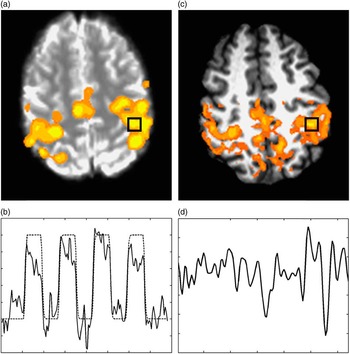
Fig. 1 a: Bilateral finger tapping task activation student’s t score, thresholded, and overlaid on BOLD-weighted EPI, the black box indicates the maximum activated region, (b) mean timeseries of the black box region in (a) superposed on the task timing (high regions are periods of finger tapping), (c) whole-brain false color map overlaid on high resolution anatomy (overlay indicates regions of high correlation to the region defined by the black box), and (d) timeseries of spontaneous BOLD fluctuations in the boxed region.

Spontaneous low-frequency oscillations have been observed in the regional cerebral blood flow and oxygenation of animals and humans using many different techniques, including laser Doppler flow (Golanov, Yamamoto, & Resi, Reference Golanov, Yamamoto and Resi1994; Hudetz, Smith, Lee, Bosnjak, & Kampine, Reference Hudetz, Smith, Lee, Bosnjak and Kampine1995), fluororeflectometry (Dora & Kovach, Reference Dora and Kovach1981; Vern, Schuette, Leheta, Juel, & Radulovacki, Reference Vern, Schuette, Leheta, Juel and Radulovacki1988), fluorescence video microscopy (Biswal & Hudetz, Reference Biswal and Hudetz1996), polarographic measurement of brain tissue (Cooper, Crow, Walter, & Winter, Reference Cooper, Crow, Walter and Winter1966; Halsey & McFarland, Reference Halsey and McFarland1974; Moskalenko, Reference Moskalenko1980), and near infrared spectroscopy (Obrig et al., Reference Obrig, Neufang, Wenzel, Kohl, Steinbrink and Einhaupl2000).

In a series of seminal studies, Biswal et al. (Biswal & Hudetz, Reference Biswal and Hudetz1996; Biswal, Hudetz, et al., Reference Biswal, Hudetz, Yetkin, Haughton and Hyde1997; Biswal, Van Kylen, et al., Reference Biswal, Van Kylen and Hyde1997; Biswal et al., Reference Biswal, Yetkin, Haughton and Hyde1995) showed that BOLD weighted MRI timeseries data contain spontaneous low-frequency fluctuations that are highly correlated between the right and left primary motor cortex while subjects are at rest. BOLD-weighted MRI allows the monitoring of hemodynamic fluctuations across the entire brain, allowing the study of low-frequency fluctuations over larger distances compared to those of optical studies. This led to many observations of synchronous fluctuations in this frequency domain in MRI timeseries acquisitions. These correlations are present between many different regions of cerebral cortex, which are part of distributed neuronal networks involved in common tasks. This synchrony has been shown to depend on the state of the brain (Lowe, Dzemidzic, Lurito, Mathews, & Phillips, Reference Lowe, Dzemidzic, Lurito, Mathews and Phillips2000).

Figure 1 shows the results of two typical resting-state fMRI studies of the cortical motor regions of the brain. The false color overlay shows regions of high temporal correlation to the very low frequency fluctuations in the left hemisphere primary motor area (black square) while subjects were resting. It is clear that the regions of highest correlation are the homologous regions in the contralateral hemisphere, as well as the medial motor regions. The source of these temporally correlated fluctuations is unknown, but is currently an area of active investigation. Biswal et al. showed that the correlations between homologous brain regions are reversibly diminished under hypercapnia, indicating that the effect is blood-flow modulated, similar to BOLD contrast (Biswal, Hudetz, et al., Reference Biswal, Hudetz, Yetkin, Haughton and Hyde1997). Furthermore, as is demonstrated by Figure 1, regions of connectivity are not confined to a single vascular distribution. In a subsequent study, Biswal et al. demonstrated that the correlation patterns from BOLD-weighted MRI data were much more similar to task-activated regions from fMRI than the correlations from strictly flow-weighted data (Biswal, Van Kylen, et al., Reference Biswal, Van Kylen and Hyde1997). The combined findings suggested that the BOLD fluctuations represent hemodynamic changes secondary to neural activity.

The precise physiological mechanisms that underlie the high correlations between functionally related brain regions are unclear. However, recent studies have shed light on the neural basis of the spatiotemporal correlations in BOLD fluctuations. These studies have provided direct evidence for neuronal signaling at or below 0.1 Hz and for the notion that spontaneous neuronal activity can reflect functional neural connectivity in the brain. Evidence for an electrophysiological basis for neuronal signaling at 0.1 Hz and below has come from an electrophysiological study conducted in nonhuman primates (Leopold, Murayama, & Logothetis, Reference Leopold, Murayama and Logothetis2003). These investigators showed that coherent fluctuations in the band-limited field potentials from neurons exist over long time scales (>10 s) and large distances (>25 mm). The band-limited potential, as defined by Leopold et al., is a measure of amplitude modulations of the power of the field potential fluctuations. The same investigators had previously shown that variations in local field potential of neurons correlates well with the BOLD signal (Logothetis, Reference Logothetis2002; Logothetis, Pauls, Augath, Trinath, & Oeltermann, Reference Logothetis, Pauls, Augath, Trinath and Oeltermann2001). Thus, this report (Leopold et al., Reference Leopold, Murayama and Logothetis2003) constitutes possible direct observation of a neuronal source of the observed low-frequency BOLD fluctuations.

Support for the notion that spontaneous neuronal activity can reflect functional connectivity came from a study of cat visual cortex using voltage sensitive dye (Kenet, Bibitchkov, Tsodyks, Grinvald, & Arieli, Reference Kenet, Bibitchkov, Tsodyks, Grinvald and Arieli2003). These investigators observed surprisingly coherent spatial patterns in spontaneous firing with no retinal input. Some of the observed patterns were identical to the cortical activation patterns observed in response to stimuli designed to activate the exposed region of cortex. The authors concluded that the spontaneous dynamically switching cortical states indicate that spontaneous neuronal behavior can reflect functional connectivity within the brain.

An additional study, which performed simultaneous EEG and fMRI in resting subjects, related spontaneous brain activity and functional connectivity (Laufs et al., Reference Laufs, Krakow, Sterzer, Eger, Beyerle, Salek-Haddadi and Kleinschmidt2003). The correlation between EEG power in various bands was mapped voxel-by-voxel to the spontaneous BOLD fluctuations. The power observed in the alpha band of the EEG data strongly correlated (inversely) to a broad network of brain regions typically associated with attentional and related cognitive processes. Additionally, positive correlations were observed between power in the beta band and BOLD fluctuations in retrosplenial, tempo-parietal, and dorsomedial prefrontal cortices. The relationship between spontaneous BOLD fluctuations and EEG power in different networks at different bands presents additional evidence to suggest that, during rest, there exist separable networks of brain regions with correlated BOLD fluctuations.

One discovery that has had major implications for the widespread adoption of rs-fMRI as a measure of functional connectivity involved the work of Raichle and colleagues (Gusnard, Akbudak, Shulman, & Raichle, Reference Gusnard, Akbudak, Shulman and Raichle2001; Raichle et al., Reference Raichle, MacLeod, Snyder, Powers, Gusnard and Shulman2001). Using quantitative positron emission tomography, they demonstrated the existence of a network of regions that consistently showed higher activity than other brain regions during the resting state. They referred to these regions as the “default mode network” (DMN). Many of these areas (posterior cingulate cortex and precuneus, medial prefrontal cortex, and angular gyrus) also showed significant deactivation during performance of specific tasks. This led to the basic postulate that the brain has a default mode of activity and performance of tasks interrupts this mode. Greicius, Krasnow, Reiss, and Menon (Reference Greicius, Krasnow, Reiss and Menon2003) provided MRI support for the Raichle et al. hypothesis by showing that two of the DMN regions (ventral anterior cingulate and posterior cingulate cortices) showed significant low-frequency BOLD correlations during rest.

Furthermore, they showed that, during execution of a cognitive task, the regions known to be involved in task performance showed inverse correlations with the posterior cingulate region. The DMN is now one of the most commonly studied resting state networks in the literature. In addition to the DMN, a very large number of additional brain networks have been identified. Cordes et al. (Reference Cordes, Haughton, Arfanakis, Wendt, Turski, Moritz and Meyerand2000) published one of the first studies to identify multiple functional networks using rs-fMRI. Since then, visual, motor, auditory, attention, and language networks, to name just a few, have been identified in the resting brain.

rs-fMRI is now the predominant method for examining functional connectivity in humans due to the ease of acquiring the data and the generality of the analyses that can be performed on these data. It is important to realize that real-world BOLD data contain various non-neuronal sources of spatiotemporal correlations that are artifactual. To draw proper conclusions, either the data must be corrected to remove these confounds or the analysis must take these confounds into account. This is accomplished either by modeling, regressing and subtracting the projected confound from the data or by including the modeled confound in the connectivity regression analysis.

Furthermore, additional data processing is used before connectivity analysis, including spatial filtering, temporal filtering, and spatial normalization. The choice of processing can have a dramatic effect on the analysis results and some processing methods that were popular in the past have been demonstrated to be associated with bias in the analysis. We note that artifact correction in fMRI and rs-fMRI data is the subject of a large body of literature. The intent of this review is to describe in general terms the most common artifacts with some basic approaches to correction. In the following paragraphs, we review analytical techniques that are necessary to remove artifacts and typical filtering techniques used to enhance the signal-to-noise ratio of the connectivity signature. Most common fMRI data analysis packages, such as AFNI, FSL, and SPM, include such correction methods.

dMRI

Diffusion MRI (dMRI) is unique in its ability to map, in vivo, the axonal connections that convey neuronal signals. As the other methods described in this article characterize correlations of neuronal activity, dMRI provides complementary information. While individual axons are too small to be resolved by dMRI, large bundles of axons such as the corpus callosum and arcuate fasciculus can be mapped across the entire brain. Analysis of these bundles, also known as fiber tracts or white matter fascicles, is used to assess structural connectivity. We will sketch the basic workings of structural connectivity analysis and highlight important caveats. Comprehensive reviews are available for further details (Johansen-Berg & Behrens, Reference Johansen-Berg and Behrens2009; Jones, Reference Jones2010; Tournier, Mori, & Leemans, Reference Tournier, Mori and Leemans2011).

dMRI measures the ease with which water moves. With appropriate mathematical modeling, an intriguing host of information can be inferred about cellular properties from dMRI data. As water moves more easily along white matter fascicles than across, dMRI can be used to infer virtual dissections of entire fasciculi throughout the brain (Catani, Howard, Pajevic, & Jones, Reference Catani, Howard, Pajevic and Jones2002). Furthermore, microstructural features such as cell dimension and shapes can, in principle, be measured (Stanisz, Szafer, Wright, & Henkelman, Reference Stanisz, Szafer, Wright and Henkelman1997). These two features of tissue, orientation and structure, are central to structural connectivity analysis. Disconnection may be related to abnormal fascicle arrangements or injury to fascicles as reflected by abnormal microstructure. However, dMRI also has fundamental limitations. This imaging method cannot indicate the polarity of axonal connections, that is, the direction of neural signals. Measures of tissue microstructure also depend heavily on the model assumptions. The measures of orientation and structure therefore lack the specificity of histological stains.

Analysis of structural connectivity is a multi-step process. First, a dMRI acquisition provides multiple images, each with a different degree of diffusion-related contrast. In diffusion tensor imaging (DTI) (Basser, Mattiello, & LeBihan, Reference Basser, Mattiello and LeBihan1994), for example, at least seven different image volumes must be acquired. Second, a model synthesizes the set of images to yield measures of tissue orientation and structure on a voxel-by-voxel basis. In DTI, fiber bundles align along the principal axis of the diffusion tensor. Demyelination and axonal loss correlate with the degree of diffusivity perpendicular to and parallel to the principal axis, respectively (Song et al., Reference Song, Sun, Ju, Lin, Cross and Neufeld2003). Third, tractography (Mori, Crain, Chacko, & van Zijl, Reference Mori, Crain, Chacko and van Zijl1999) takes the orientation information from each voxel and generates streamlines that represent long-range axonal connections between cortical regions. Finally, structural connectivity among different cortical regions can be assessed by counting the number of streamlines of a given pair of regions (Hagmann et al., Reference Hagmann, Kurant, Gigandet, Thiran, Wedeen, Meuli and Thiran2007).

The basic sketch of steps outlined above provides a framework for understanding the enormous literature describing current research. First, dMRI acquisitions place strong demands on imaging hardware due to the duration of the scan, strong diffusion-weighting gradients and echo-planar imaging readout used to limit the duration of the scan. Quality control must be implemented to ensure that the imaging data are not corrupted by artifact (Oguz et al., Reference Oguz, Farzinfar, Matsui, Budin, Liu, Gerig and Styner2014; Tournier et al., Reference Tournier, Mori and Leemans2011). Unfortunately, erroneous conclusions may result entirely from image artifacts. The strong gradients induce strong vibrations that can shake electronic components that may be loose on the MR scanner, leading to spikes and increased levels of noise. If, for example, the spikes occur during the latter half of a longitudinal study, an increase in variance may be detected that results entirely from image artifact.

Cardiac gating has been recommended to avoid pulsatility artifact, particularly in periventricular and brain stem regions (Skare & Andersson, Reference Skare and Andersson2001). A fingertip pulse plethysmograph is typically used. Such triggering, however, may fail among patients with compromised circulation to the extremities. One inherently difficult problem is motion. dMRI is, by design, sensitive to the motion of water. This sensitivity makes dMRI particularly susceptible to large amounts of head motion. If one group of subjects moves more than another (e.g., patient group greater than control subjects), artifactual between group differences may be detected (Yendiki, Koldewyn, Kakunoori, Kanwisher, & Fischl, Reference Yendiki, Koldewyn, Kakunoori, Kanwisher and Fischl2013).

Among models, the diffusion tensor (Basser et al., Reference Basser, Mattiello and LeBihan1994) is most widely used. As the model requires only six diffusion-weighted image volumes and one image without diffusion weighting, the acquisition time can be as short as 1 min. However, at least 30 diffusion-weighted image volumes are recommended to limit within subject noise in diffusivity measurements (Jones, Reference Jones2004). From the tensor, one can derive several scalar summary parameters that can be used to assess tissue on a voxel-by-voxel basis. The principal eigenvector of the tensor can be associated with the orientation of white matter fibers in a voxel. Diffusivity along the principal eigenvector, called longitudinal or axial diffusivity, can correlate with axonal fragmentation. Diffusivity perpendicular to the principal eigenvector, called transverse or radial diffusivity, can correlate with demyelination. However, such interpretation depends highly on the injury or disease (Budde et al., Reference Budde, Kim, Liang, Schmidt, Russell, Cross and Song2007) and breaks down at locations with crossing fibers (Wheeler-Kingshott & Cercignani, Reference Wheeler-Kingshott and Cercignani2009). The variance among diffusivities is described by fractional anisotropy (FA). Reduced FA is typically interpreted as reduced tissue integrity, but has been found to behave counter to expectations in the presence of crossing fibers (Douaud et al., Reference Douaud, Jbabdi, Behrens, Menke, Gass, Monsch and Smith2011).

The limitations of the tensor model have stimulated a plethora of alternative models (Assemlal, Tschumperle, Brun, & Siddiqi, Reference Assemlal, Tschumperle, Brun and Siddiqi2011) to more accurately capture the complexity of tissue structure. Crossing fibers have received much attention because modeling enables tractography of a wider variety of white matter fascicles than is otherwise possible (Behrens, Berg, Jbabdi, Rushworth, & Woolrich, Reference Behrens, Berg, Jbabdi, Rushworth and Woolrich2007). More recent work aims to quantify cellular properties such as axon diameters (Assaf, Blumenfeld-Katzir, Yovel, & Basser, Reference Assaf, Blumenfeld-Katzir, Yovel and Basser2008) and gliosis (Wang et al., Reference Wang, Wang, Haldar, Yeh, Xie, Sun and Song2011). These models require more extensive and demanding image acquisitions than the diffusion tensor model, resulting in long scans and more stringent hardware requirements. Computation time to fit the models can also be problematically long. The comparison of these models against quantitative histology (Barazany, Basser, & Assaf, Reference Barazany, Basser and Assaf2009; Wang et al., Reference Wang, Wang, Haldar, Yeh, Xie, Sun and Song2011) is more limited than for the diffusion tensor, hampering interpretation.

Tractography essentially works by connecting principal eigenvectors from diffusion tensors of contiguous voxels (Basser, Pajevic, Pierpaoli, Duda, & Aldroubi, Reference Basser, Pajevic, Pierpaoli, Duda and Aldroubi2000; Conturo et al., Reference Conturo, Lori, Cull, Akbudak, Snyder, Shimony and Raichle1999; Mori, Crain, Chacko, & van Zijl, Reference Mori, Crain, Chacko and van Zijl1999), resulting in three-dimensional maps of white matter fascicles (Catani et al., Reference Catani, Howard, Pajevic and Jones2002). By accounting for crossing fibers, otherwise occult fascicles can be identified (Behrens et al., Reference Behrens, Berg, Jbabdi, Rushworth and Woolrich2007). Tractography has been used to investigate Wallerian degeneration. Pierpaoli et al. (Reference Pierpaoli, Barnett, Pajevic, Chen, Penix, Virta and Basser2001) showed that white matter connected to, but distal from, an infarct demonstrated abnormal diffusivity consistent with injury. Furthermore, measures of tissue integrity along specific fiber pathways can correlate with functional disability (Lowe et al., Reference Lowe, Horenstein, Hirsch, Marrie, Stone and Bhattacharyya2006) and with resting-state connectivity (Lowe et al., Reference Lowe, Beall, Sakaie, Koenig, Stone, Marrie and Phillips2008, Reference Lowe, Koenig, Beall, Sakaie, Stone, Bermel and Phillips2014).

EEG/MEG Coherence

Cortical electrical or magnetic fluctuations can be measured noninvasively with EEG or MEG sensors placed on or above the scalp, respectively. EEG and MEG are important tools for functional connectivity analysis since they provide a direct measure of cortical synaptic activity with high temporal resolution. Additionally, EEG and MEG provide complementary measures of functional connectivity, as EEG is preferentially sensitive to radially oriented cortical sources and MEG is sensitive to tangential sources (Cohen & Cuffin, Reference Cohen and Cuffin1983).

The functional connectivity of different cortical regions is often examined in the context of amplitude and phase similarities between signals derived from multiple EEG or MEG sensors. These similarities can be quantified statistically using coherence, that is, the squared cross spectrum between two signals normalized by the power spectrum of each signal (Bendat & Piersol, Reference Bendat and Piersol2000). Conceptually, coherence represents the ratio of the squared covariance of two signals and the variance of each signal, that is, a squared correlation coefficient, providing a measure of the percentage of variance within a signal accounted for by a linear transformation of another signal (Nunez & Srinivasan, Reference Nunez and Srinivasan2006). Increases in coherence between signals derived from EEG or MEG sensors may arise due to distributed cortical interactions, revealing functionally connected brain networks that emerge at the time scales of perceptual and cognitive events (Buzsaki, Reference Buzsaki2006; Engel, Fries, & Singer, Reference Engel, Fries and Singer2001).

Within EEG or MEG multi-sensor recordings, it is important to consider whether coherence results from genuine cortical interrelationships or whether it results due to sensor pairs measuring activity from common sources. EEG potentials are spatially smeared by the volume conduction properties of the head, resulting in inflated coherence between EEG sensors within ~10 cm (Srinivasan, Winter, Ding, & Nunez, Reference Srinivasan, Winter, Ding and Nunez2007). MEG signals are unaltered by volume conduction, but measure from common sources due to magnetic field spread (Brookes et al., Reference Brookes, Hale, Zumer, Stevenson, Francis, Barnes and Nagarajan2011). These issues are attenuated when spatial filtering and source modeling approaches are applied to estimate the distribution of cortical source potentials that contribute to MEG and EEG sensor measurements (for reviews, see Michel et al., Reference Michel, Murray, Lantz, Gonzalez, Spinelli and Grave de Peralta2004; Schoffelen & Gross, Reference Schoffelen and Gross2009). These approaches may complement each other in functional connectivity analysis, revealing coherent patterns that emerge at different spatial scales and source orientations (Nunez et al., Reference Nunez, Silberstein, Shi, Carpenter, Srinivasan, Tucker and Wijesinghe1999, Reference Nunez, Srinivasan, Westdorp, Wijesinghe, Tucker, Silberstein and Cadusch1997).

Seed-Based Analyses

The earliest observations of resting-state functional connectivity were made using what is now termed seed-based correlation (Biswal et al., Reference Biswal, Yetkin, Haughton and Hyde1995; Lowe, Mock, & Sorenson, Reference Lowe, Mock and Sorenson1998). These were serendipitous observations made while studying the noise characteristics of BOLD-weighted MRI timeseries data. Model-based methods, which provide more statistical power and cleaner hypothesis testing, are still very limited to this day due to the fact that there is no “signal” that characterizes the connectivity signature in resting state data, unlike activation-based fMRI. Seed-based correlation analysis remains a very popular technique for analyzing rs-fMRI data. The approach allows the investigator to interrogate the spatial regions of the brain that have a significant temporal correlation to the spontaneous BOLD fluctuations in a pre-specified seed region. In this section, we review typical analysis issues associated with performing seed based analysis of BOLD-weighted MRI timeseries data obtained during the resting state.

Seed-based correlation requires the selection of a seed region, whose connectivity to the rest of the brain is of interest. This is best done with activation-based fMRI using a task related to the function of interest. For example, connectivity related to hand motor function can be examined by acquiring both a resting state scan and a functional hand motor task activation scan (Lowe et al., Reference Lowe, Mock and Sorenson1998). The functional scan is used to localize function in the primary motor cortex and a seed region is determined from an activation map (see Figure 1). The mean timeseries in the resting state data averaged over several voxels around the seed region is used to estimate the spontaneous fluctuations in that region.

The use of anatomic localization alone has been shown to be problematic at providing reliable resting state networks (Cole, Smith, & Beckmann, Reference Cole, Smith and Beckmann2010). However, there have been many studies of resting state networks that have been done using anatomic localization, most notably studies of the default mode network (Greicius et al., Reference Greicius, Krasnow, Reiss and Menon2003). The problem is related to that described above when discussing group analyses. Spatial variation in the localization of function can vary considerable across subjects, especially in cortical regions. As with group voxel-level analyses, this is typically addressed by using spatial smoothing. A data-driven method was recently introduced to combine anatomic localization with functional information present in the resting data itself to refine the seed location to improve the robustness of network identification (Lowe et al., Reference Lowe, Koenig, Beall, Sakaie, Stone, Bermel and Phillips2014). This obviates the need for spatial smoothing.

There are three types of seed-based analyses that are common in the literature: (1) simple Pearson correlation of the seed-derived timeseries with all voxels in the brain, (2) frequency domain analysis of all voxels compared to seed-derived timeseries (Yang et al., Reference Yang, Long, Yang, Yan, Zhu, Zhou and Gong2007), and (3) inter-regional connectivity analyses to determine local interconnectivity (Zang, Jiang, Lu, He, & Tian, Reference Zang, Jiang, Lu, He and Tian2004). The first is the most common technique and will be described briefly here. The other methods are beyond the scope of this brief introduction to seed-based connectivity analyses and are mentioned for completeness.

Pearson correlation analysis involves calculating the normalized projection of a reference vector (i.e., seed voxel-derived timeseries) with another vector (i.e., timeseries from any give voxel). It can be expressed as:

where $\vec {x}$ is the timeseries at a given voxel and $\vec {x}$ _ref is the timeseries from the reference, or seed, region. A whole-brain map of this correlation can be produced. A threshold can be applied based on a desired false positive rate and rendered onto high resolution anatomy for display purposes (see Figure 1). Note that the Pearson correlation coefficient has an algebraic relationship to a Student’s t (Press, Teukolsky, Vetterling, & Flannery, Reference Press, Teukolsky, Vetterling and Flannery1993). Correlation coefficients are intuitive for assessing the level of alignment of the signals, but Student’s t’s are more intuitive for understanding the significance, or p-value, of the result.

Complex Network Analyses

Complex network analyses of human whole-brain structural and functional imaging data sets emerged approximately a decade ago (Achard, Salvador, Whitcher, Suckling, & Bullmore, Reference Achard, Salvador, Whitcher, Suckling and Bullmore2006; Bassett, Meyer-Lindenberg, Achard, Duke, & Bullmore, Reference Bassett, Meyer-Lindenberg, Achard, Duke and Bullmore2006; Eguiluz, Chialvo, Cecchi, Baliki, & Apkarian, Reference Eguiluz, Chialvo, Cecchi, Baliki and Apkarian2005; Gong et al., Reference Gong, He, Concha, Lebel, Gross, Evans and Beaulieu2009; Hagmann et al., Reference Hagmann, Cammoun, Gigandet, Meuli, Honey, Wedeen and Sporns2008; He, Chen, & Evans, Reference He, Chen and Evans2007; Iturria-Medina, Sotero, Canales-Rodriguez, Aleman-Gomez, & Melie-Garcia, Reference Iturria-Medina, Sotero, Canales-Rodriguez, Aleman-Gomez and Melie-Garcia2008; Liu et al., Reference Liu, Liang, Zhou, He, Hao, Song and Jiang2008; Stam, Reference Stam2004; Stam, Jones, Nolte, Breakspear, & Scheltens, Reference Stam, Jones, Nolte, Breakspear and Scheltens2007), in parallel with increasing conceptualization of the brain as a complex network of brain regions and interregional structural and functional associations (Bullmore & Sporns, Reference Bullmore and Sporns2009). Analyses of complex brain networks have coalesced around the notion of the connectome, defined as the complete organizational description of anatomical brain connections (Sporns, Reference Sporns2012; Sporns, Tononi, & Kötter, Reference Sporns, Tononi and Kötter2005) and more loosely extended to encompass organizational descriptions of complex brain functional connections, as well descriptions of complex brain connectivity in neurological and psychiatric disorders (Calhoun, Miller, Pearlson, & Adalı, Reference Calhoun, Miller, Pearlson and Adalı2014; Kopell, Gritton, Whittington, & Kramer, Reference Kopell, Gritton, Whittington and Kramer2014; Rubinov & Bullmore, Reference Rubinov and Bullmore2013).

Complex brain networks represent the organization of whole-brain white-matter pathways, or whole-brain functional coactivation patterns and typically comprise hundreds of brain regions (vertices or nodes) and thousands of interregional connections (edges or links). As a rule of thumb, networks are deemed to be complex if their organization cannot be adequately described with visualizations (Newman, Reference Newman2010). Complex brain networks contrast with other network models in cognitive neuroscience, which associate with a specific function (such as language), have few nodes, and are easily described with visualizations (Fox & Raichle, Reference Fox and Raichle2007).

Accurate definition of nodes in complex brain networks is an important problem, and affects the meaningfulness and interpretability of subsequent network analyses (Rubinov & Sporns, Reference Rubinov and Sporns2010). Nodes should ideally be functionally homogeneous, spatially contiguous, cover the whole-brain, have high signal-to-noise ratio, and be reproducible between subjects (Craddock et al., Reference Craddock, Jbabdi, Yan, Vogelstein, Castellanos, Di Martino and Milham2013; Thirion, Varoquaux, Dohmatob, & Poline, Reference Thirion, Varoquaux, Dohmatob and Poline2014). Most current atlases are based on structural (e.g., cytoarchitectonic or transcriptomic) or functional (e.g., regional activity patterns) datasets, but no atlas simultaneously fulfils all the above criteria. High resolution structural or functional imaging may allow the appearance of such gold-standard reference atlases in the next couple of decades (Amunts et al., Reference Amunts, Lepage, Borgeat, Mohlberg, Dickscheid, Rousseau and Evans2013; Insel, Landis, & Collins, Reference Insel, Landis and Collins2013).

Accurate definition of structural or functional brain connections is likewise an important problem, with similar implications for meaningfulness and interpretability. Anatomical connections typically represent white-matter tracts and are inferred with diffusion MRI and tractography or less directly with gray-matter-thickness covariance methods (Alexander-Bloch, Giedd, & Bullmore, Reference Alexander-Bloch, Giedd and Bullmore2013; Behrens & Sporns, Reference Behrens and Sporns2012; Evans, Reference Evans2013; Hagmann et al., Reference Hagmann, Cammoun, Gigandet, Gerhard, Grant, Wedeen and Sporns2010). Functional connections reflect patterns of statistical associations, irrespective of underlying anatomical connectivity, and are inferred with statistical measures such as the Pearson or partial correlation coefficients, mutual information, and lag-based measures such as Granger causality (Smith et al., Reference Smith, Miller, Salimi-Khorshidi, Webster, Beckmann, Nichols and Woolrich2011; Van Dijk et al., Reference Van Dijk, Hedden, Venkataraman, Evans, Lazar and Buckner2010). Bayesian network inference methods are used infrequently due to large network sizes, although methodological and computational progress may make these methods more relevant in the future (Seghier & Friston, Reference Seghier and Friston2013). Connections may have additional properties of directionality (afferent or efferent), weight (strong or weak), and sign (positive or negative) (Rubinov & Sporns, Reference Rubinov and Sporns2011).

Analysis of complex brain networks leverage methods which have origins in graph-theoretical analyses of social networks, but have been extensively and inter-disciplinarily expanded in the last two decades to describe properties of complex real-life systems in diverse scientific fields (Boccaletti, Latora, Moreno, Chavez, & Hwang, Reference Boccaletti, Latora, Moreno, Chavez and Hwang2006; Newman, Reference Newman2003). Broadly, such analyses are divided into analyses of global, intermediate or local network organization. Analyses of global organization describe properties of the whole network, analyses of intermediate network organization describe properties of groups of nodes in the network, and analyses of local network organization describe properties of individual nodes.

Analyses of global network organization typically describe the propensity for whole-brain functional specialization and functional integration. Functional specialization is inferred as the extent to which network nodes form clusters and is computed with measures such as the clustering coefficient (the average number of triangles as a fraction of all connected triplets). Functional integration is measured as the propensity of the network for global interconnectedness and is computed with measures such as the characteristic path length (the average length of shortest paths between all pairs of nodes). The simultaneous presence of functional specialization and integration (relative to random control networks) defines a measure of small-world-ness, a non-specific marker of complex brain network organization (Bassett & Bullmore, Reference Bassett and Bullmore2006; Humphries & Gurney, Reference Humphries and Gurney2008; Watts & Strogatz, Reference Watts and Strogatz1998).

Analyses of intermediate network organization typically partition the network into communities or modules, functionally specialized and densely interconnected groups of nodes, and are conceptually similar to independent components analysis (see below) and other clustering methods (Girvan & Newman, Reference Girvan and Newman2002; Meunier, Lambiotte, & Bullmore, Reference Meunier, Lambiotte and Bullmore2010). Analyses of intermediate network organization may also bipartition the network into a central and dense group of “core” or “rich-club” nodes and a sparsely interconnected group of peripheral nodes (Colizza, Flammini, Serrano, & Vespignani, Reference Colizza, Flammini, Serrano and Vespignani2006; van den Heuvel & Sporns, Reference van den Heuvel and Sporns2011). Importantly, unlike global and local measures of complex network organization, detection of community (and to a lesser extent core-periphery) structure often involves the use of non-deterministic optimization algorithms which may produce many possible solutions (Csermely, London, Wu, & Uzzi, Reference Csermely, London, Wu and Uzzi2013; Fortunato, Reference Fortunato2010).

Analyses of local network organization typically quantify the importance of individual nodes in the network. Importance is a subjective notion, but is most commonly defined using measures such as degree (the total number of nodal connections), participation coefficient (the diversity of nodal connections), and the betweenness centrality (fractions of all shortest path traversing the node). The robust detection of hub nodes is a notable strength of complex network analysis and such hubs are increasingly implicated in diverse neurological and psychiatric disorders (Crossley et al., Reference Crossley, Mechelli, Scott, Carletti, Fox, McGuire and Bullmore2014; Harrington et al., Reference Harrington, Rubinov, Durgerian, Mourany, Reece, Koenig and Rao2015; Stam, Reference Stam2014; van den Heuvel & Sporns, Reference van den Heuvel and Sporns2013).

The combined global, intermediate and local analyses of complex brain networks provide a comprehensive statistical description of structural and functional organization of the human brain. Inevitably, however, the quality and interpretation of such descriptions relies on the quality of the underlying brain imaging and on adequate definitions of nodes and connections. Increasing spatial and temporal resolution of human imaging is likely to move the analysis and interpretation of complex brain networks closer to biological processes underlying normal and abnormal brain structure, activity and function.

Independent Components Analysis (ICA)

ICA is a statistical method used to discover hidden factors (sources or features) from a set of measurements or observed data such that the sources are maximally independent. Within the context of neuroimaging, the algorithm has been widely implemented on EEG data, identifying independent time courses (for a review, see Eichele, Calhoun, & Debener, Reference Eichele, Calhoun and Debener2009; Makeig, Debener, Onton, & Delorme, Reference Makeig, Debener, Onton and Delorme2004) or on fMRI data, emphasizing independent spatial maps (for a review, see Calhoun & Adali, Reference Calhoun and Adali2012). We focus here on fMRI, where ICA reduces the original (voxels×time) observations into a linear mixture of spatially independent brain maps (components) and associated time courses (mixing matrix).

Since the model identifies latent fMRI sources whose voxels have the same time course, each component can be considered a measure of the degree to which each voxel is functionally connected (or correlated) to the component time course. These correlated patterns of activity likely result from activity within somewhat distinct brain modes or sources, which motivates their description as distinct brain networks with potentially distinct properties. For example, the statistical maps generated from cognitive tasks with general linear modeling (GLM) resemble fMRI source maps, even when derived from data collected in the absence of an explicit task (Calhoun & Allen, Reference Calhoun and Allen2013; Calhoun, Kiehl, & Pearlson, Reference Calhoun, Kiehl and Pearlson2008; Smith et al., Reference Smith, Fox, Miller, Glahn, Fox, Mackay and Beckmann2009).

The fMRI source spatial profile depends in part on the model order (i.e., the number of components estimated), with higher model orders resulting in a more detailed parcellation of distinct areas (Abou-Elseoud et al., Reference Abou-Elseoud, Starck, Remes, Nikkinen, Tervonen and Kiviniemi2010; Allen et al., Reference Allen, Erhardt, Damaraju, Gruner, Segall, Silva and Calhoun2011). Spatial maps also depend on the particular algorithm implemented in the ICA decomposition (for details on ICA algorithms see Hyvarinen, Karhunen, & Oja, Reference Hyvarinen, Karhunen and Oja2001; Stone, Reference Stone2004). For example, the Infomax algorithm can emphasize sparse independent fMRI maps, which aligns with the assumption of sparse and distributed cognitive activations, and the sparse and spatially specific artifacts that result from motion and cardiac activity (McKeown et al., Reference McKeown, Makeig, Brown, Jung, Kindermann, Bell and Sejnowski1998).

While there is considerable utility in conducting ICA at the subject level, it is difficult to identify common sources across subjects when performing the subsequent group analysis. To address this problem, extensions have been developed to incorporate information from multiple subjects within a single ICA decomposition (Beckmann & Smith, Reference Beckmann and Smith2005; Calhoun & Adali, Reference Calhoun and Adali2012; Calhoun, Adali, Pearlson, & Pekar, Reference Calhoun, Adali, Pearlson and Pekar2001; Esposito et al., Reference Esposito, Scarabino, Hyvarinen, Himberg, Formisano, Comani and Salle2005; Guo & Pagnoni, Reference Guo and Pagnoni2008; Schmithorst & Holland, Reference Schmithorst and Holland2004), as implemented within GIFT Matlab software (http://mialab.mrn.org/software/gift) and in MELODIC software (http://www.fmrib.ox.ac.uk/fsl/). Following group ICA, individual subject time courses may be derived by back-reconstructing the group components onto the individual subject data, generating subject specific images and time courses for each component (Calhoun et al., Reference Calhoun, Adali, Pearlson and Pekar2001; Erhardt et al., Reference Erhardt, Rachakonda, Bedrick, Allen, Adali and Calhoun2011).

While ICA provides a useful data-driven decomposition of functionally distinct networks, many cognitive processes emerge from the collective activity of multiple brain networks (Siegel, Donner, & Engel, Reference Siegel, Donner and Engel2012; Varela, Lachaux, Rodriguez, & Martinerie, Reference Varela, Lachaux, Rodriguez and Martinerie2001). Thus, there is considerable motivation in examining network interactions via associations among the time courses of networks derived from ICA. These interactions are revealed in part by examining cross-correlations between network or component time courses, resulting in a (component×component) cross-correlation matrix which represents the degree of associations among networks, or the functional network connectivity (FNC) (Jafri, Pearlson, Stevens, & Calhoun, Reference Jafri, Pearlson, Stevens and Calhoun2008). Group ICA is an important processing step within FNC analysis, since it reduces the original (voxels×voxels) cross-correlation matrix into a more tangible (components×components) matrix that compares the relationship between the individual back-reconstructed time courses (see Figure 2).

Fig. 2 Examples of within and among network connectivity information. The left panel shows brain regions parcellated from resting fMRI data using group ICA and the right panel shows the functional network connectivity matrix among these regions (cross-correlation).

Cross-correlations are examined either across the entire component time course, revealing static or aggregate measures of connectivity, or within shorter segments, revealing time-varying changes in dynamic FNC (Allen et al., Reference Allen, Damaraju, Plis, Erhardt, Eichele and Calhoun2014; Chang & Glover, Reference Chang and Glover2010; Sakoğlu et al., Reference Sakoğlu, Pearlson, Kiehl, Wang, Michael and Calhoun2010). Static connectivity provides an approximate measure of functional associations across the entire time course, but is insensitive to dynamic changes in connectivity patterns which may emerge at shorter time scales (for a review, see Hutchison et al., Reference Hutchison, Womelsdorf, Allen, Bandettini, Calhoun, Corbetta and Chang2013). Thus, FNC matrices may be calculated from successive ~40- to 60-s intervals and partitioned into groups of recurring connectivity patterns using multivariate approaches such as k-means clustering (Allen et al., Reference Allen, Damaraju, Plis, Erhardt, Eichele and Calhoun2014; Damaraju et al., Reference Damaraju, Allen, Belger, Ford, McEwen, Mathalon and Calhoun2014; Rashid, Damaraju, Pearlson, & Calhoun, Reference Rashid, Damaraju, Pearlson and Calhoun2014; Sakoğlu et al., Reference Sakoğlu, Pearlson, Kiehl, Wang, Michael and Calhoun2010), ICA (Yaesoubi, Miller, & Calhoun, Reference Yaesoubi, Miller and Calhoun2015) or singular value decomposition (svd) (Leonardi, Shirer, Greicius, & Van De Ville, Reference Leonardi, Shirer, Greicius and Van De Ville2014). Many of these approaches implicitly assume that there are a handful of distinct connectivity patterns (i.e., states), that a single state is present at any given time, and that states recur over minute-to-minute intervals. It will be important for future research to evaluate these assumptions. For example, a recent study suggests that dynamic FNC patterns were better described by overlapping states during rest, but by distinct states during tasks (i.e., silently counting, singing, or recalling events) (Leonardi et al., Reference Leonardi, Shirer, Greicius and Van De Ville2014).

Dynamic FNC analysis may compliment static FNC measures, each capturing different characteristics of network dynamics. For example, while static FNC provides an aggregate measure of connectivity, dFNC provides a parcellation into distinct states which can be characterized by the frequency and duration of occurrence (Calhoun et al., Reference Calhoun, Miller, Pearlson and Adalı2014). For example, individuals diagnosed with schizophrenia demonstrate a reduced presence of network connectivity states comprised of large-scale connectivity patterns. These patterns are characterized by increased connectivity among and across visual and somatosensory areas, and decreased connectivity among those regions and regions implicated in cognitive control, that is, the supramarginal gyrus, precuneus, middle frontal gyrus, inferior frontal gyrus, cingulate gyrus, and inferior parietal lobule (Damaraju et al., Reference Damaraju, Allen, Belger, Ford, McEwen, Mathalon and Calhoun2014).

These dynamics were obscured when comparing static connectivity differences between these patients and controls. The reduction of large-scale connectivity within schizophrenia could potentially underlie many symptoms, including the attention and perceptual deficits associated with the disorder (for a review, see Heinrichs & Zakzanis, Reference Heinrichs and Zakzanis1998; Mesholam-Gately, Giuliano, Goff, Faraone, & Seidman, Reference Mesholam-Gately, Giuliano, Goff, Faraone and Seidman2009). Thus, there is considerable utility in examining static and dynamic FNC among group ICA time courses and it will be important for further research to examine the correspondence between these patterns and distinct cognitive processes (Calhoun et al., Reference Calhoun, Miller, Pearlson and Adalı2014).

dMRI

Maps of whole-brain anatomic connectomes have been proposed to assess whole-brain patterns of connectivity (Hagmann et al., Reference Hagmann, Kurant, Gigandet, Thiran, Wedeen, Meuli and Thiran2007). The anatomic connectomes demonstrate consistency in terms of scan-rescan reproducibility, correlation with resting-state functional connectivity, and bilateral symmetry. However, these anatomic connectomes likely leave out several important connections, particularly those that traverse fiber crossings, for example, transcallosal connections between hand regions in motor cortex (Hagmann et al., Reference Hagmann, Cammoun, Gigandet, Meuli, Honey, Wedeen and Sporns2008).

An important open question is the definition of anatomic connectivity. Fiber counts from streamline tractography are commonly used to represent anatomic connectivity. However, every tractography algorithm depends on several adjustable parameters. A slight adjustment of any of these can drastically change the fiber count. Measures of tissue integrity along a pathway can be used as an alternative to fiber counts and have been found to relate favorably to functional connectivity (Lowe et al., Reference Lowe, Koenig, Beall, Sakaie, Stone, Bermel and Phillips2014). Tract-based spatial statistics (TBSS) (Smith et al., Reference Smith, Jenkinson, Johansen-Berg, Rueckert, Nichols, Mackay and Behrens2006) adopts the latter approach to assess tissue injury, but does not use tractography to identify white matter fascicles. Rather, a scalar fractional anisotropy map is used in conjunction with an atlas to identify the fascicles, completely avoiding the algorithmic instabilities associated with tractography. However, the regions identified by TBSS do not directly relate to cortical regions. More recent work involving the TRActs Constrained by UnderLying Anatomy (TRACULA) software (Yendiki et al., Reference Yendiki, Panneck, Srinivasan, Stevens, Zollei, Augustinack and Fischl2011) involves a registration-based approach, but constrains analysis to a limited set of well-defined and reliable pathways, thus representing only a small fraction of the total pathways in the brain.