
I. INTRODUCTION
Frank Dunstone Graham (1890–1949) conducted research on international values since the 1920s and published his most important book, The Theory of International Values, in Reference Graham1948,Footnote 1 the year before his accidental death.Footnote 2 In this book, he made two important contributions to trade theory. The first contribution was the construction of multi-country, multi-commodity trade models and the derivation of their equilibrium solutions. The second was his discovery of the significance of link commodities for trade theory.Footnote 3 Whereas the first contribution is recognized generally, the second accomplishment has not been generally accepted. In fact, it has been almost completely forgotten.Footnote 4
Link commodities are those produced in common in more than one country—for example, cars produced in Japan, the US, and Germany; IT products produced in China, Korea, and Japan; and beef produced in Brazil, Australia, and the US. Graham developed a new trade theory by ranking link commodities as the most important concept. This new theory thoroughly criticized John Stuart Mill’s theory of reciprocal demand (Mill Reference Mill1852, Bk. 3, ch. 18) and Alfred Marshall’s idea of the “offer curve” (Marshall [1879] Reference Marshall and Groenewegen1997, pp. 83–112; Marshall Reference Marshall1923, pp. 330–360) or “representative bales” (Marshall Reference Marshall1923, p. 157), which were mainstream trade theories at the time.
However, Graham’s criticism of Mill and Marshall was not widely supported. Soon after the publication of Graham (Reference Graham1948), many book reviews and papers on the subject of Graham’s trade theory were written, and most did not agree with his criticism. G. Alexander Elliot, in a long and favorable review (Elliot Reference Elliott1950), attempted to demonstrate that Graham’s two-country, multi-commodity cases can be translated into offer curves by using Marshall’s concept of representative bales, and did not approve of Graham’s neoclassical trade theory criticism. Lloyd Metzler (Reference Metzler1950) recognized Graham’s theory to be innovative (p. 304) and valid (p. 312) but did not acknowledge Graham’s criticism, and asserted that a synthesis of Graham’s ideas and classical doctrines would ultimately be possible (Reference Elliott1950, p. 313). Thomson Whitin (Reference Whitin1953) made a comparison between Graham’s analysis and classical reciprocal supply and demand analysis, and wrote that although Graham’s analysis showed a necessity to substantially revise or extend classical analysis in some respects, many of the differences were of a semantic nature, and, therefore, a synthesis of the two analyses is possible (Reference Whitin1953, p. 520). Lionel W. McKenzie explained the structure of the Graham model analytically and proved the existence and uniqueness of an equilibrium in multi-country, multi-commodity, one-factor trade models, wherein Graham’s model is included (McKenzie Reference McKenzie1954a, Reference McKenzie1954b). However, he denied Graham’s assertion that the existence of “limbo” prices (as in the Mill case, described later) was quite improbable (McKenzie Reference McKenzie1954a, pp. 176–177). James Melvin (Reference Melvin1969), like Elliot, also attempted to interpret Graham’s model based on offer curves. John S. Chipman, in his mid-1960s trade theory survey, evaluated Mill highly and severely criticized Graham (Chipman Reference Chipman1965, pp. 493–501). Prior to these comments, Jacob Viner (Reference Viner1937) had also criticized Graham and supported Mill and Marshall (pp. 448–453, 535–555).
Although Graham’s theory could be understood to a certain extent during the 1950s, since then it has gradually disappeared from researchers’ sight, due to a few reasons. First, the synthesis of Graham and Mill–Marshall was conducted only in two-country, multi-commodity cases (Elliot Reference Elliott1950; Whitin Reference Whitin1953) or multi-country, two-commodity cases (Whitin Reference Whitin1953), and was, moreover, biased toward Mill–Marshall. In fact, synthesis was never conducted in multi-country, multi-commodity cases. Shortly, Graham was substantially confined in the Mill–Marshall framework, leading to an underestimation of link commodities and Graham (see below, section III).
Second, Graham did not show how to derive his equilibrium solution from given conditions; rather, he presented only the calculation results of his numerical examples. Moreover, he could not prove the existence and uniqueness of an equilibrium.Footnote 5 Although, as mentioned above, McKenzie proved its existence and uniqueness, he also did not present the methodology for practically deriving the equilibrium solution.
Third, many researchers perceived the existence of link commodities in the real trading world as quite a rare phenomenon. In fact, even before Graham, several economists had referred to the possibility of the existence of commodities produced in common in more than one country: for example, Patrick Stirling ([1853] Reference Stirling1969, pp. 211–242); Hans von Mangoldt ([1863] Reference von Mangoldt1975); Henry Sidgwick (Reference Sidgwick1887, pp. 205–209); Francis Ysidro Edgeworth (Reference Edgeworth1894, pp. 619–621, 630–634); J. Shield Nicholson (Reference Nicholson1897, pp. 301–310); and C. Francis Bastable (Reference Bastable1903, p. 43).Footnote 6 However, they, with the exception of Stirling and Sidgwick,Footnote 7 did not realize link commodities’ innovative significance for trade theory. For example, Edgeworth (Reference Edgeworth1894) believed that standard commodities (link commodities, in our terms) were hypothetical, and even if they existed, they would most likely be insignificant (p. 634). Chipman (Reference Chipman1965) also described the following contents: there must be more commodities than countries in order for link commodities to exist, but there is a natural tendency for the number of commodities to be less than or equal to the number of countries, considering that we can group commodities whose absolute advantages are approximately equal and whose elasticities of substitution are relatively high in one category (p. 500).
In this study, we present a method for practically deriving the equilibrium solution using a modified version of Graham’s model and clarify the relationships between the equilibrium solutions and given conditions in numerical simulations. Moreover, we show that the probability of link commodities’ existence is very high and that perfect specializations seldom appear. In addition, we describe important matters concerning relative wage rates that Graham did not explicitly discuss in his theory of international values.
The remainder of this paper is organized as follows. In section II, we introduce the essence of Graham’s theory of international values, since the theory is relatively obscure. In section III, we present a modified Graham model and explain the method for deriving equilibrium solutions. In section IV, we explore the probabilities of various patterns of the international division of labor. In section V, we conduct numerical simulation using a three-country, four-commodity numerical example, in which we specifically focus on the relationship between wage rates and patterns of the international division of labor and on the effect on wage rates of changes in production techniques. In section VI we present concluding remarks.
II. GRAHAM’S THEORY OF INTERNATIONAL VALUES
The Fundamental Structure of Graham’s Model
We can summarize the fundamental structure of Graham’s model as follows:Footnote 8
#1. There are many countries and many commodities.
#2. There are no intermediate goods and no profits. All commodities are for consumption.
#3. For each country, constant opportunity costs, economic scales, and demand structures are given.
#4. Full employment and trade equilibrium (in other words, the equivalence of each country’s national expenditures and national incomes) are fulfilled.
#5. There are no transport costs and no trade barriers.
Under these assumptions, patterns of the international division of labor (hereafter, IDL patterns), international values, and each country’s volumes of production, exports, imports, and consumption are uniquely determined.
Graham explained the above through the presentation of many numerical examples, but without any mathematical treatment. Although, prior to Graham, Hans von Mangoldt ([1863] Reference von Mangoldt1975) already derived equilibrium solutions for two-country, multi-commodity cases, in multi-country, multi-commodity cases, some possible IDL patterns were barely demonstrated, at best.Footnote 9 Indeed, Graham was the first to present the existence of equilibrium solutions in multi-country, multi-commodity (four-country, three-commodity or ten-country, ten-commodity) cases.Footnote 10
We explain the three given conditions of #3 in more detail below.
Production techniques of commodities are expressed by means of opportunity costs, not by labor costs. According to Graham, each country’s production techniques differ in every sector. While classical economists express the difference between these techniques by the difference in their labor input coefficients, Graham expresses it using the difference between the opportunity costs of each commodity. Concretely, he designates a specific commodity as a benchmark commodity (for which the opportunity cost is 1) and expresses the production techniques of other commodities by the number of units producible by giving up the production of one unit of the benchmark commodity. The opportunity costs are essentially constant.Footnote 11 He describes the reason for using opportunity costs as follows:
When we think in terms of opportunity cost it can be conclusively demonstrated that Ricardo, Mill, and the neoclassicists, were wholly wrong in supposing that the same rule, which regulates the relative value of commodities in one country does not regulate the relative value of the commodities exchanged between two or more countries. (Graham Reference Graham1948, p. 333)
The economic scale of each country is expressed by the maximum production volumes of the benchmark commodity, which is realized when each country specializes in the commodity. Although full employment is assumed, the volumes of production factors and absolute productivity levels are not given. Therefore, differentials in per capita income or wage rates among countries are not directly argued in the theory of international values and are instead treated as another problem.Footnote 12 Graham’s strong adherence to the belief that the rule regulating domestic values and the rule regulating international values must be identical prevented him from making another contribution to trade theory. If he had selected labor costs instead of opportunity costs to express production techniques, he could have provided important findings on the relationship between IDL patterns and relative wage rates, as we show in this study.
The demand structure of each country is given by the expenditure coefficients (the proportion of amounts expended on each commodity in total expenditures). The sum of the coefficients is 1 (i.e., all income is expended for consumption) in every country. We must note that Graham did not ignore the function of demand in the determination of international values and that the demand, however, was not “reciprocal national demand” but “total world demand for the various products” (Graham Reference Graham1948, pp. 16, 263).
Determination of International Values
International values, or the world relative prices of commodities, are determined not by reciprocal national demand but by opportunity costs in each country, just like domestic values. The most important aspect in this determination is the existence of commodities produced in common in more than one country, which are termed link commodities (Graham Reference Graham1948, pp. 254, 332).Footnote 13 Link commodities link the opportunity costs of countries that produce the same link commodities, meaning that the relative prices of all commodities produced in these countries are determined uniquely. In principle, every country has at least one link commodity, suggesting that plural link commodities exist in the world at large. Consequently, a body of link commodities interconnects the opportunity costs of all countries and thus determines the international values of all commodities worldwide. Link commodities are, in turn, determined through the interactions of opportunity costs, economic scales, and demand structures in each country. According to Graham, link commodities were the missing link in the classical theory of international values (Reference Graham1948, p. 252) and the greatest obstacle to discovering this missing link was “mortmain derived mainly from J. S. Mill,” that is, the paradigm of thinking within only the two-country, two-commodity framework (Reference Graham1948, p. 27).
Stability of the International Values Determined
International values, once formed, exhibit a high level of stability in the presence of shifts in demand. Such shifts are adjusted through changes in production volumes and import-export volumes without price changes. If drastic shifts in demand do occur, prices might change slightly. In this case, these price changes are necessarily accompanied by changes in the IDL pattern. Newly formed international values are also based on the linkage of opportunity costs in each country.
However, depending on the three given conditions of #3 above, the linkage between opportunity costs might become disconnected. Graham called such a state of disconnection “limbo,” in which case a small demand shift induces an immediate change in international values. This is the case to which Mill’s theory of reciprocal demand applies.Footnote 14 Graham regarded it as highly improbable without solid grounds and substantially ignored it. Ironically, Graham’s behavior paralleled that of his critics; he ignored the limbo case, just as his critics ignored the linkage case, with both justifying their neglect by appealing to the presumed empirical irrelevance of the neglected phenomena. Unlike Graham and his critics, in this paper, we derive the conditions that give rise to both the linkage and the limbo cases.
III. MODIFIED GRAHAM MODEL AND THE DERIVATION OF EQUILIBRIUM SOLUTIONS
Model Setting and Definition of Terms
First, we modify Graham’s original model and set the modified version, which we call the “Graham type trade model.”
1. There are M countries and N commodities. M and N are integers that are more than 2 and N is larger than M.Footnote 15
2. There are no intermediate goods and no profits. All commodities are for consumption.
3. Full employment and trade equilibrium (that is, the condition of national expenditures equaling national income in each country) are both fulfilled.
4. There are no transport costs and no trade barriers.
5. There are no international movements of labor and the domestic wage rate is equal in all sectors.
6. For each country, the production techniques expressed by constant labor input coefficients,Footnote 16 the quantities of available labor, and the demand structures expressed by expenditure coefficients are given. Although we do not absolutely require information about the labor input coefficients of some sectors (e.g., the automotive industry in developing countries or the crude oil extraction industry in non-oil-producing countries) in which the probability of being internationally competitive is almost zero, we nonetheless provide the coefficients of all sectors for convenience of explanation. We assume that the degrees of comparative advantage between any two countries selected arbitrarily differ for every sector. The sum of the expenditure coefficients is 1 in every country.
Under these assumptions, the IDL patterns, international values, wage rates in each country, and each country’s volumes of production, exports, imports, and consumption are determined uniquely. Before explaining the determination logic and the method for deriving the equilibrium solution, we will define some terms.
First, the equilibrium solution consists of the identification of the IDL pattern, each commodity’s equilibrium production volumes in each country, each country’s equilibrium wage rates, and the equilibrium international values. By obtaining the equilibrium solution, we can then calculate the volumes of exports, imports, and consumption of all commodities in each country.
Given the international division of labor, some sectors in each country continue production activity while other sectors cease activity. We call the former active points and the latter non-active points. IDL patterns must be reasonable. Here, “reasonable” means a situation in which both conditions, “production costs of active points = commodity prices” and “production costs of non-active points > commodity prices,” are fulfilled.
Since the purpose of an economic model is to enable understanding of the real world, let us observe the actual situation regarding the international division of labor. Then, we can observe a scene that does not exist in ordinary trade models, that is, the fact that some commodities are produced in common in more than one country: for instance, cars produced in Japan, the US, and Germany; textile products in some developing countries, and so on. We call such commodities link commodities after the work of Graham. Link commodities determine the relative wage rates of all the countries producing the same link commodities, thereby determining the relative production costs of all active and non-active points in these countries. As the same commodity has an identical price in every country, the relative labor productivities (or, the inverses of the labor input coefficients) of link commodities are precisely identical with the relative wage rates,Footnote 17 and the relative production costs are obtained by multiplying the relative wage rates by constant labor input coefficients.
Countries with the same link commodities are directly connected. However, countries can also be indirectly linked. Suppose that among countries A, B, and C, countries A and B both produce the same link commodity, and B and C produce a different link commodity in common. In this case, all three countries are interlinked, although A and C are not directly but rather indirectly (via the medium of B) linked. Hereafter, the term “link” means not only “linked directly” but also “linked indirectly” and we use the term “linkage” to express “the state of being linked.”
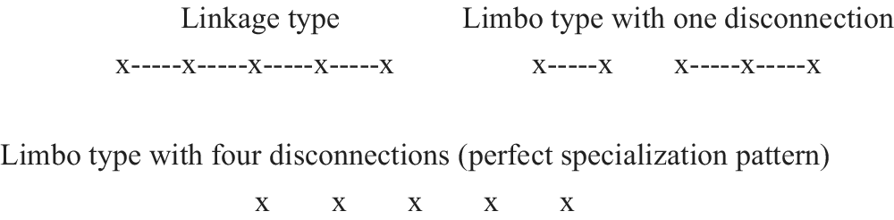
IDL patterns can be classified as one of two types. First, when all countries are linked through link commodities, then this pattern is called the linkage type. In this type, by setting an adequate numéraire, the wage rates of all countries, all commodity prices (= the production costs of active points), and the production costs of all non-active points can be expressed by labor input coefficients according to each IDL pattern. In other words, once the IDL patterns are determined, all wage rates and commodity prices (hereafter, the wage rates/prices) are determined by the patterns themselves, i.e., there is a one-to-one correspondence between IDL patterns and the wage rates/prices.
The second type of IDL pattern is called the limbo type, in which the linkage of countries is imperfect and one or more disconnections in the linkage occur. Therefore, determining all wage rates/prices using only IDL patterns is impossible. Theoretically, this disconnection can occur in the range from 1 to M–1. When there are M–1 disconnections, perfect specialization patterns (hereafter, PSPs) are formed, which have no link commodities and are ordinary textbook cases of the two-country, two-commodity trade model, wherein each country specializes in a commodity with a comparative advantage. An ordinary case in a two-country, two-commodity model is an extreme case in a multi-country, multi-commodity model, as we will demonstrate later.
Figure 1 illustrates these two IDL pattern types through a five-country case. Five countries (expressed by x) are all linked in the linkage type, whereas in one of the limbo types, the linkage is disconnected in one place. The five countries are divided into two groups, within which more than one country is linked. The other limbo type is a PSP and all constituent countries are disconnected. We need to pay attention that there are intermediate IDL patterns between the linkage type and the PSPs and that in these intermediate patterns, there necessarily exist one or more linkages. This intermediate situation never emerges in the two-country cases.

Figure 1. Examples of the Two Types of IDL Patterns
Thus, to discuss Graham’s model in the framework of two-country or two-commodity cases may be accompanied by the oversight of some important matters, so we will provide another example of the oversight. Metzler (Reference Metzler1950, p. 318) wrote as follows: “Graham did not attach sufficient importance to the possible magnitude of movements in the terms of trade between industrial countries and producers of primary products.” However, in the multi-country, multi-commodity case, this statement is incorrect. If a developed country and an emerging country are linked directly and if the emerging country is linked directly to a developing country, then the developed country and the developing country are linked indirectly. Thus, it is sufficiently possible that industrial countries and even least developed countries are linked indirectly, if not directly. In that case, the terms of trade between industrial products and primary products would be fixed.
Derivation of the Equilibrium Solution for the Linkage Type
Here, we explain a method to derive the equilibrium solution for the linkage type practically. This process comprises three steps as follows: searching for and identifying reasonable IDL patterns (Step 1), setting up simultaneous equations according to each IDL pattern and solving them mathematically (Step 2), and selecting an economically meaningful solution set (Step 3). We describe the details consecutively from Step 1 through Step 3 below.
Step 1. We have to search for and identify the reasonable IDL patterns classified into the linkage type. Whether an IDL pattern is reasonable or not is determined only by labor input coefficients, and the judgment of reasonableness is simple, albeit laborious. Provided that all the countries produce at least one commodity and that all the commodities are produced, the number of possible IDL patterns is (M^[N–1]) (N^[M–1])Footnote 18 in an M-country, N-commodity case: if M is 3 and N is 4, the number is 432. As commodity prices and production costs of all non-active points are already known in every pattern, we only have to compare commodity prices with production costs. Almost all of these patterns are not reasonable, and the number of reasonable patterns is (M+N–2)!/([M–1]![N–1]!): if M is 3 and N is 4, this number is 10.Footnote 19 If M and N are large, because of the large number of IDL patterns to be judged, it is difficult to even identify reasonable patterns. Including the rest of this process, the support of a computer program is required to perform the calculations.
Step 2. For all reasonable patterns, we formulate simultaneous equations, which are composed of M equations expressing the full employment conditions of each country and N equations expressing the supply-demand balance for each commodity. However, the independent equations are M+N–1, because one of the N equations is not independent, owing to Walras’s law. The unknowns are the production volumes at each active point, the number of which is M+N–1 for the linkage type (McKenzie Reference McKenzie1954a, p. 175). The reason that the number is M+N–1 is as follows. There must be N active points to ensure that all commodities are produced. In this situation, all countries are entirely unconnected. Therefore, to link all countries, M–1 additional active points are needed. This means that the number of link commodities is the number of countries minus 1. Thus, as the equations and unknowns are equal in number, we can solve all sets of equations mathematically. We provide an example of a three-country, four-commodity case in Appendix 1.
However, whether the solutions calculated mathematically are meaningful economically is another problem, which necessitates the next process.
Step 3. Since production volumes must be positive economically, we have to select a set such that all solutions are positive from the (M+N–2)!/([M–1]![N–1]!) sets of solutions. If such a set exists, its solutions would be the equilibrium solution required. Accordingly, the IDL pattern, production volumes, and wage rates/prices are determined. Further, the consumption volumes and import-export volumes for each country can also be easily calculated.
Derivation of the Equilibrium Solution in the Limbo Type
If, in all of the linkage type IDL patterns, there is no set such that all solutions are positive, it means that one or more disconnections of the linkage have occurred. Then, we must widen the search range to find the equilibrium solution to limbo type IDL patterns. The process consists of three steps (steps 4 to 6) as follows.
Step 4. Same as for the linkage type, we have to identify the reasonable patterns of the limbo type. The number of patterns is very large:
∑(M+N–l–2)!/{(M–l–1)!(N–l–1)!l!} (l = 1, 2, …, M–1)Footnote 20
If M is 3 and N is 4, the number is 15.
Similarly, in the case of the limbo type, whether a pattern is reasonable is determined only by the labor input coefficients. However, because not all the wage rates/prices are determined according to IDL patterns, we have to adopt a different approach from the linkage type. There are two different methods, as follows.
We will explain those methods for the case of IDL patterns with l disconnections. In this case, countries are divided into l + 1 groups (see Figure 1) and the patterns have to be reasonable within each group as well as among groups. Reasonableness of the patterns within each group can be checked easily because linkage determines the relative wage rates. A condition exists for the IDL patterns among groups to be reasonable. That is, the relative wage rates between countries belonging to different groups have to be within a specific range to be reasonable. This constraint condition relating to wage rates has to be satisfied between all combinations of two out of the l + 1 groups, or there are l+1C2 constraint conditions relating to wage rates. If wage rates that satisfy all of these conditions can exist under an IDL pattern, this IDL pattern is then judged as reasonable (we show some examples in section IV, section V, and Appendix 2). Contrarily, if these conditions contradict each other, the IDL pattern is judged as not reasonable. For convenience of explanation, we describe this method accompanied by identification of the range of wage rates as judging method 1.
The other method, called judging method 2, uses the identified IDL patterns of the linkage type. If, while holding the condition that all commodities are produced and all countries produce at least one commodity, we remove one active point of a linkage type IDL pattern, then one disconnection occurs and a limbo type IDL pattern with one disconnection is derived. Further, by adding the same operation to this newly obtained pattern, we can obtain an IDL pattern with two disconnections. By repeating the same operation up to M–1 disconnections, we can identify all limbo type IDL patterns (we show an example in section V).
Step 5. After identifying the patterns, we formulate equations and solve them. When the number of disconnections is l, l +1 country groups are formed. While the wage rates/prices within each country group are determined by the IDL pattern itself, those between groups are not determined by only the pattern. To determine all wage rates/prices, we have to add the wage rate of a country in each group, excluding the group to which a country producing a numéraire commodity belongs, as the unknown.Footnote 21 The number of additional unknowns is l. On the other side, the number of active points reduces by the number of disconnections, or l, in the limbo type (McKenzie Reference McKenzie1954a; see the above-mentioned judging method 2 to understand intuitively). Eventually, regardless of the number of disconnections, the total unknowns are still M+N–1, and we can mathematically solve all sets of equations. We provide an example of a three-country, four-commodity case in Appendix 2.
Step 6. Finally, we have to select a set of solutions that fulfills the following two conditions: all solutions are positive and the obtained wage rates are within the adequate range in the case of using the judging method 1, or the solution set passes a competitiveness test in the case of judging method 2. This test is conducted to check whether non-active points are competitive or not, by comparing the production costs of non-active points with commodity prices. As the entire wage rates/prices are already obtained in Step 5, the test is quite simple. If at least one non-active point is competitive, then the set is disqualified. Of course, the verification of the wage rates’ range and the competitiveness test are equivalent. In any case, only one set satisfies these two conditions and this set is the equilibrium solution.
IV. THE PROBABILITIES OF IDL PATTERNS: THE GRAHAM CASE VERSUS THE MILL CASE
The IDL patterns formed depend on labor input coefficients, quantities of available labor, and expenditure coefficients. Here, we investigate the probabilities of the IDL patterns. Because it is very complicated and difficult to explain them analytically in the case of more than two countries, we use a two-country (A and B), three-commodity (1, 2, and 3) example. Notations a ij (> 0), b j (> 0: Σb j =1), L i (> 0), p j, w i, and x ij mean commodity j’s labor input coefficient in country i, commodity j’s expenditure coefficient in common in both countries, quantities of available labor in country i, commodity j’s price, wage rate of country i, and commodity j’s production volumes in country i, respectively. The numéraire is commodity 1. For simplicity, we suppose:
a B1/a A1 > a B2/a A2 > a B3/a A3
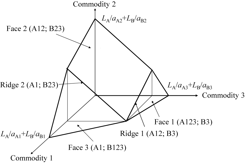
Then we can identify five reasonable IDL patterns, namely, (A123; B3), (A12; B3), (A12; B23), (A1; B23), and (A1; B123): here, for example, (A123; B3) means that country A produces commodities 1, 2, and 3, and country B produces commodity 3. Three are linkage type and two are limbo type (and PSPs because of the two-country case). Figure 2 illustrates the world production possibility frontier (hereafter, WPPF) of this example.

Figure 2. World Production Possibility Frontier
Three faces represent the linkage type IDL patterns, and two ridges are the limbo type IDL patterns. As long as production points lie on the same faces, the wage rates/prices do not change, and only production volumes change. The reason is that the link commodity does not change. On the ridges, the price adjustments responding to shifts in demand are conducted.
We can learn the conditions in which each IDL pattern is formed by following the aforementioned steps 2 and 3 in the case of linkage type and steps 5 and 6 in the case of limbo type. First, let us examine the conditions when the pattern (A123; B3) is formed. In this pattern, p 1=1, p 2=a A2/a A1, p 3=a A3/a A1, w A=1/a A1, and w B=a A3/(a B3a A1). The conditions of full employment and supply-demand balance (only two of the three are independent) are as follows:
a A1x A1+a A2x A2+a A3x A3 = L A
a B3x B3 = L B
x A1p 1 = w AL Ab 1 + w BL Bb 1
x A2p 2 = w AL Ab 2 + w BL Bb 2
x A3p 3+x B3p 3 = w AL Ab 3 + w BL Bb 3
When all the solutions are positive, this pattern is formed. It is obvious that x A1, x A2, and x B3 are positive, but it is unclear whether x A3 is positive or not. By solving the above equations for x A3, we obtain x A3 = L Ab 3/a A3 – (1– b 3)L B/a B3; accordingly, x A3 > 0 ⇔ L B/L A<{b 3/(1 − b 3)}(a B3/a A3). Therefore, if L B/L A<{b 3/(1 − b 3)}(a B3/a A3), the pattern (A123; B3) is formed.
Next, we examine the pattern (A12; B3). In this pattern, p 1=1, p 2=a A2/a A1, and w A=1/a A1; p 3 (= w Ba B3) and w B are unknown. The conditions of full employment and supply-demand balance are as follows:
a A1x A1 + a A2x A2 = L A
a B3x B3 = L B
x A1p 1 = w AL Ab 1 + w BL Bb 1
x A2p 2 = w AL Ab 2 + w BL Bb 2
x B3p 3 = w AL Ab 3 + w BL Bb 3
Conditions for forming this pattern are:
x A1, x A2, x B3 > 0
a A3/(a B3a A1) > w B > a A2/(a B2a A1)Footnote 22
By solving the above equations for w B, we obtain:
w B = (L A/L B){b 3/(1 − b 3)}/a A1
Because this value of w B (> 0) ensures x A1, x A2, x B3 > 0, by substituting this value into the above inequality, we obtain the conditions for forming the pattern (A12; B3) as follows:
{b 3/(1 − b 3)}(a B3/a A3) < L B/L A <{b 3/(1 − b 3)}(a B2/a A2)
Likewise, we can derive the conditions for the remaining three patterns. Figure 3 depicts these results.
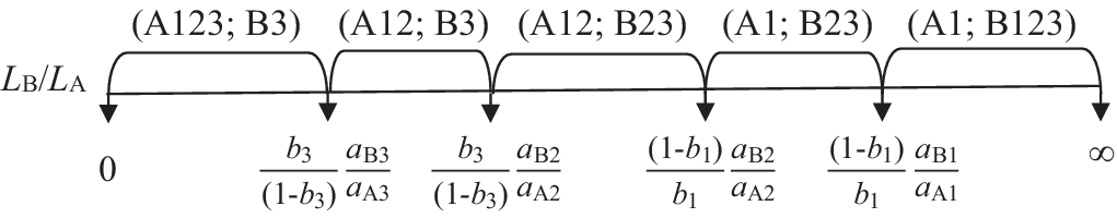
Figure 3. Conditions for Forming Each IDL Pattern
This figure shows that we can calculate the probability of the IDL patterns by defining the range of the relative labor quantities of country B and providing the labor productivity differentials (LPD) of each sector and the expenditure coefficients. If we assume that the range of L B/L A is from 0 to 10, a B1/a A1 is 4, a B2/a A2 is 3, a B3/a A3 is 2, and the expenditure coefficients are all 1/3, then the probability of the limbo type is 25%. If the range of L B/L A is from 1 to 8, within which both countries do not fail to gain from trading—in other words, if the patterns (A123; B3) and (A1; B123) are excluded—the probability is roughly 36%. Figure 3 also shows that the smaller the LPD’s differences between sectors are, the higher the probability of the linkage type. The differences are expressed by angles between two faces in Figure 2, and a large angle means a large difference between the LPDs. Expenditure coefficients also affect the probability. If, for example, b 2 is larger (b 1 and b 3 are smaller), the probability of the pattern (A12; B23) increases; i.e., the probability for commodities with a larger expenditure coefficient to become link commodities increases.
Even though we cannot diagram the case of more than three commodities, as we can imagine easily, with increases in the number of countries and commodities, the differences would become smaller, and, therefore, the probability of the linkage type would increase. Increases in the number of countries also decrease the probability of the PSPs rapidly because the number of constraint conditions relating wage rates increases rapidly. If five or ten countries exist, for the PSPs to be formed, ten (5C2) or forty-five (10C2) constraint conditions have to be fulfilled. When the three givens are arbitrarily set, the possibility that all the constraint conditions are met would be extremely low if not zero.Footnote 23
We will call the aspect of quantity adjustments without price changes the Graham case and the aspect of adjustments with price changes the Mill case. Then, the linkage type is exclusively the Graham case, the limbo type other than PSPs is the coexistence of the Graham and Mill cases, and PSPs are exclusively the Mill case. Therefore, in the multi-country, multi-commodity trade models, the Graham case overwhelms the Mill case.
V. ANALYSIS OF THE MODEL USING A NUMERICAL EXAMPLE
Identification of Reasonable IDL Patterns
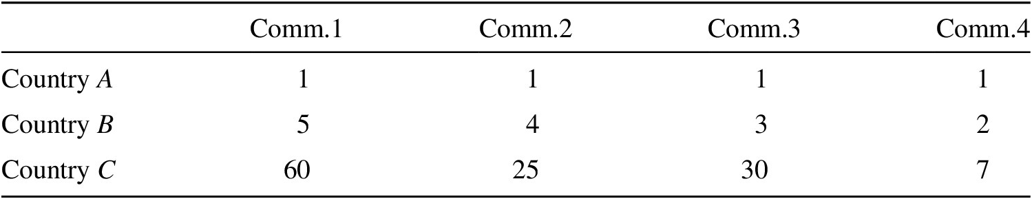
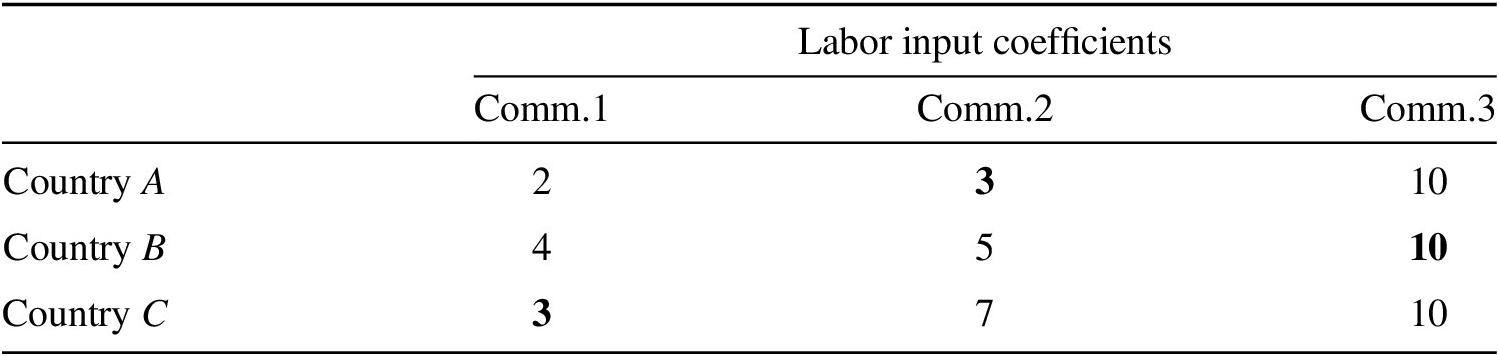
We set a three-country, four-commodity numerical example and analyze the characteristics of the Graham type trade model by observing changes in the equilibrium values arising from changes in the given conditions. Table 1 presents the labor input coefficients. Here, country A symbolizes a developed country, country B represents an emerging country, and country C represents a developing country. Units of commodities are chosen in a manner that all the labor input coefficients of country A are 1, and the commodities are numbered in order of country A’s diminishing comparative advantage between countries A and B. Footnote 24 Labor input coefficients of country C are given arbitrarily. The numéraire is commodity 1.
Table 1. Labor Input Coefficients

Based on Table 1, ten linkage type IDL patterns are determined as shown below. The first parentheses show the IDL patterns, the second are commodity prices in order from commodity 1 to 4, and the third show wage rates from country A to C.
Linkage type IDL patterns
4+1+1 type (one country produces four commodities and the other two produce one commodity each)
1) (A1234; B4; C4) (1; 1; 1; 1) (1; 1/2; 1/7)
2) (A1; B1234; C4) (1; 4/5; 3/5; 2/5) (1; 1/5; 2/35)
3) (A1; B1; C1234) (1; 25/60; 1/2; 7/60) (1; 1/5; 1/60)
3+2+1 type (one country produces three commodities, another country produces two, and a third country produces one)
4) (A123; B34; C4) (1; 1; 1; 2/3) (1; 1/3; 2/21)
5) (A123; B3; C24) (1; 1; 1; 7/25) (1; 1/3; 1/25)
6) (A1; B123; C24) (1; 4/5; 3/5; 28/125) (1; 1/5; 4/125)
7) (A12; B234; C4) (1; 1; 3/4; 1/2) (1; 1/4; 1/14)
8) (A13; B3; C234) (1; 5/6; 1; 7/30) (1; 1/3; 1/30)
9) (A1; B13; C234) (1; 1/2; 3/5; 7/50) (1; 1/5; 1/50)
2+2+2 type (all the countries produce two commodities each)
10) (A12; B23; C24) (1; 1; 3/4; 7/25) (1; 1/4; 1/25)
Next, the limbo type IDL patterns are presented. The IDL patterns and wage rates (including their ranges) are shown below (commodity prices are omitted). In patterns with two disconnections, country C needs to fulfill two wage rates constraints. For example, (1; 1/4–1/3; 1/25–1/7, w B/10–2w B/7) means that country A’s wage rate is 1; country B’s wage rate is more than 1/4 and less than 1/3; country C’s wage rate is more than 1/25 and less than 1/7, and more than 1/10 and less than 2/7 of country B’s wage rate.
Limbo type IDL patterns with one disconnection
11) (A123; B4; C4) (1; 1/3–1/2; 2w B/7) 12) (A12; B34; C4) (1; 1/4–1/3; 2w B/7)
13) (A1; B234; C4) (1; 1/5–1/4; 2w B/7) 14) (A1; B23; C24) (1; 1/5–1/4; 4w B/25)
15) (A1; B3; C234) (1; 1/5–1/3; w B/10) 16) (A12; B3; C24) (1; 1/4–1/3; 1/25)
17) (A13; B3; C24) (1; 1/3; 1/30–1/25) 18) (A1; B123; C4) (1; 1/5; 4/125–2/35)
19) (A1; B1; C234) (1; 1/5; 1/60–1/50) 20) (A123; B3; C4) (1; 1/3; 1/25–2/21)
21) (A1; B13; C24) (1; 1/5; 1/50–4/125) 22) (A12; B23; C4) (1; 1/4; 1/25–1/14)
Limbo type IDL patterns with two disconnections (these are PSPs)
23) (A12; B3; C4) (1; 1/4–1/3; 1/25–1/7, w B/10–2w B/7)
24) (A1; B23; C4) (1; 1/5–1/4; 1/60–1/7, 4w B/25–2w B/7)
25) (A1; B3; C24) (1; 1/5–1/3; 1/60–1/25, w B/10–4w B/25)
From this list, we can confirm that there is one (1+1C2) wage rates constraint in the limbo type patterns with one disconnection and three (2+1C2) with two disconnections. We also provide concrete examples of the judging method 2. We can derive, for example, pattern 11) by removing A4 from pattern 1). In the same way, 11) or 12) is derived by removing B3 or A3 from 4), 23) by removing B4 from 12), and so on.
Furthermore, by focusing on the wage rate of 11), which is derived from 1) and 4), we observe that it lies between those of 1) and 4). Such a relation of derivation and wage rates suggests that, for instance, 1) and 4) adjoin each other and 11) forms the boundary between 1) and 4) on the WPPF. According to Yoshinori Shiozawa (Reference Shiozawa, Shiozawa, Oka and Taichi2017a, pp. 5–6), the WPPF of the multi-country, multi-commodity case has a convex polytope shape, which is covered by ten facets in a three-country, four-commodity case. Each facet represents each IDL pattern of the linkage type, and the joints of the facets represent the IDL patterns of the limbo type. In two-dimensional graphs of two-country (or multi-country) two-commodity cases, the lines correspond to the linkage type patterns and the vertexes represent the limbo type patterns. In three-dimensional graphs of two-country, three-commodity cases, the faces are facets and correspond to the linkage type patterns, and the ridges are joints and represent the limbo type patterns.Footnote 25
On closer examination of these patterns, we can see that there are many cases where some active points do not follow the grades of comparative advantage between two countries. For example, although country B’s commodity 4 is the lowest comparative advantage between countries B and C, country B produces only commodity 4 together with country C in the patterns 1) and 11). Simple relationships between two countries disappear behind complicated relationships among three countries. This fact is widely known since Ronald Jones (Reference Jones1961).Footnote 26
Wage Rates and Link Commodities: The Missing Link in Graham’s Theory
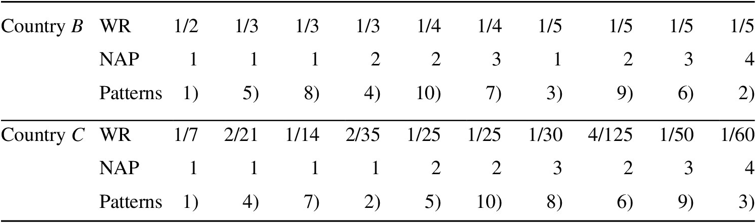
As country A’s wage rate is always 1, we compile the wage rates of only countries B and C in Table 2 by limiting to the linkage type. Wage rates (WR in the table) are arranged in decreasing order, and the number of active points (NAP) and IDL patterns (Patterns) are also shown.
Table 2. Wage Rates, Number of Active Points, and IDL Patterns

There are very large wage differentials according to the IDL patterns. The range of the differentials reaches out from the minimum to maximum of the productivity differentials of individual sectors, namely from 1/2 to 1/5 between countries A and B, from 1/7 to 1/60 between countries A and C, and from 2/7 to 5/60 between countries B and C, which can be easily calculated from Table 2. This stems from the fact that, as mentioned in section III, wage rate differentials are equal to productivity differentials of link commodities, and all the commodities have a possibility to become link commodities when only production techniques are given or before quantities of available labor and demand structures are given.
Generally, similarly to two-country cases, the fewer the NAP, the more advantageous the WR is. However, some phenomena that never emerge in two-country cases are observed. First, there are four patterns with the same WR of 1/5, which is the most disadvantageous for country B in comparison with country A, and, besides, the NAP in these patterns varies from 1 to 4. The reason is that although these patterns are different from each other, the link commodity connecting countries A and B is the same, namely, commodity 1, in which country B has the greatest comparative disadvantage with respect to country A. Especially, Pattern 3) or (A1; B1; C1234) is of interest. When country C produces all the commodities, countries A and B specialize in the production of the commodity of their greatest comparative advantage with respect to country C. Accidentally, the commodity is most comparatively disadvantageous for country B with respect to country A.
Second, though the patterns that countries B and C produce only one commodity are four, respectively, country C’s WRs are all different and country B’s WRs are among three of four. In all the patterns, both countries must select the most advantageous sector for themselves. However, the sector varies according to the IDL patterns.
Third, the WR differentials between countries A and C are different among nine of ten patterns in spite of the four-commodity model. The reason is diversity of the linkage patterns between both countries: five are direct linkages and the remaining five indirect linkages.
Last, we assume that the expenditure coefficient of commodity 2 increases drastically and that of commodity 3 decreases drastically in countries A and B, and, consequently, the IDL pattern changes from 4) or (A123; B 34; C4) to 7) or (A12; B234; C4). Then, the wage rate of country B declines from 1/3 to 1/4 and, simultaneously, that of country C from 2/21 to 1/14, notwithstanding that the three givens of country C do not change at all. The reason is that countries B and C are still linked by the same commodity. As a result, commodity terms of trade for country C deteriorate to country A. Note that the national reciprocal demand, in Mill’s terminology, between countries A and C remains unchanged.Footnote 27
Graham discovered the significance of the link commodities for trade theory. However, because he discussed his theory of international values based on opportunity costs, he could not develop the theory on wage rates sufficiently. The relation between wage rates and link commodities was the missing link in Graham’s theory of international values.
Shifts in Demand, IDL Patterns, and Wage Rates
Now, we observe the movement of equilibrium solutions induced by changes in expenditure coefficients. Labor input coefficients are the same as shown in Table 1. Country A has 500 labor, country B has 2000, and country C has 4000. Each country’s expenditure coefficients are equal for each commodity: those of commodities 2 and 3 are fixed at 0.20; those of commodities 1 and 4 change by 0.01 from 0.01 to 0.59. Then, the transition of IDL patterns and wage rates is as follows. Only expenditure coefficients of commodity 1 are shown and those of commodity 4 (0.6 – expenditure coefficients of commodity 1) are omitted.

The starting point is Pattern 4). From here, demand for commodity 1 wherein country A has competitiveness increases, and demand for commodity 4 wherein countries B and C have competitiveness decreases. Until expenditure coefficients of commodity 1 reach 0.13, this pattern is maintained, and therefore prices/wage rates are unchanged and the quantity adjustments, or the Graham case, continue. Meanwhile, country A increases the production and export of commodity 1, decreases the production and export of commodity 3, and decreases the import of commodity 4. Country B increases the production and export of commodity 3, decreases those of commodity 4, and increases the import of commodity 1. Country C increases the import of commodity 1 and increases the export of commodity 4.
When the coefficients reach 0.13, country A can no longer increase the production of commodity 1, owing to the labor quantity constraints: because A is the only country producing commodity 2 and world demand for commodity 2 is unchanged, country A cannot decrease the production of commodity 2. Thus, quantity adjustments between country A and countries B and C become non-functional and the IDL pattern switches to Pattern 12). In this pattern, price adjustments, or the Mill case, continue between country A and both countries. Between B and C, however, the Graham case is still effective. Under the Mill case, wage rates of both B and C continue to decline, and when the coefficients reach 0.19, the production of commodity 2 in country B become competitive, leading to Pattern 7). What brings Pattern 12) to an end is the wage rates constraints.
After this, similar processes follow and Pattern 6) is the final point. In every switch of IDL pattern, what causes the disconnection of linkages, including the switch from 22) to 24), is always labor quantity constraints, and what causes linkages, including the switch from 24) to 14), is always wage rates constraints. In the above example, the PSP, namely Pattern 24) appears, where the Mill case holds exclusively. In the other patterns except for this special case, either the Graham case holds exclusively or it is effective together with the Mill case. Although we intentionally selected the above example accompanied by the PSP, the PSPs seldom appear ordinarily, that is, under the condition that the three givens are arbitrarily provided. Even in the above example, the probability of the linkage type accounts for more than 70% (0.43/0.60) and the Graham case nearly 80% (0.43/0.60 + 0.09/0.60/2).
Pay attention that switching runs along mutually resembling patterns without a jump, and that changes in wage rates on the occasion of the switch are small. This suggests that the equilibrium solutions move on adjoining facets or their joints covering the WPPF by responding to small and continuous changes in expenditure coefficients. As long as shifts in demand are small, either wage rates/prices do not change at all or the changes are small.
Changes in Production Techniques and Wage Rates/Prices
Here, we describe the effects of changes in production techniques on wage rates/prices.Footnote 28 Suppose that the IDL pattern 10) (A12; B23; C24) is formed. Commodity 2 is the common link commodity among three countries, with wage rates (1; 1/4; 1/25) and commodity prices (1; 1; 3/4; 7/25).
When the labor productivity of commodity 4 in country C doubles (the labor input coefficient halves), the price of commodity 4 halves. Country C’s real wage rate certainly increases due to the decline in commodity 4’s price, but this is common with the other countries in which labor productivity does not increase at all. This is not a good result for country C. In short, relative wage rates are unchanged. The results of increases in the labor productivity of commodities produced in only the home country leak into foreign countries.Footnote 29
On the contrary, increases in labor productivity of link commodities raise the home countries’ wage rates. Increases in wage rates, in turn, raise the production costs of commodities whose increases in labor productivity are lower than those of the link commodities. Suppose that the labor productivity of commodity 2 in country C increases and consequently country C’s wage rate increases. Then, two consequences are possible. First, commodity 4 made in country C maintains competitiveness despite the price increases, and the commodity terms of trade of both countries A and B deteriorate. Second, commodity 4 made in country C loses its competitiveness, and some IDL patterns having been not reasonable thus far, e.g., (A12; B234; C2) or (A123; B34; C2), newly acquire reasonableness, leading to changes in the IDL pattern.
If changes in production techniques occur in plural sectors of plural countries, and thereby the structure of international competitiveness changes widely, the IDL pattern and the wage rates/prices would also change widely. Unlike shifts in demand structures, changes in production techniques are always drastic and necessarily change wage rates/prices. Changes in production techniques are the very driving force of structural change in the world economy.
VI. CONCLUDING REMARKS
The most important key phrase for the Graham type trade model is “link commodities.” These commodities, during demand shifts, perform quantity adjustments without price changes or the Graham case. Nowadays, many firms that produce commodities with high supply elasticity conduct quantity adjustments in the presence of demand shifts. Except for primary commodities with low supply elasticity, many firms revise commodity prices only when they experience a change in production costs. The Graham type trade model is compatible with such a reality. At present, however, trade theories focusing on the PSPs and price adjustments or the Mill case are dominant. We need to rid ourselves of this undue emphasis on the PSPs and price adjustments.
Another dominant tendency in contemporary trade theory is the emphasis on intra-industry trade. With the development of world trade statistics after World War II, the existence of commodities produced in common in more than one country has been recognized. However, these commodities have not been treated as link commodities but have been discussed within the framework of intra-industry trade or differentiated products (Grubel Reference Grubel1967; Krugman Reference Krugman1980). Trade models based on differentiated products are substantially one-sector models and, therefore, do not have generality. If trade of the products with decreasing costs were general, many trade theories would lose their foundations. Furthermore, there are intra-industry trade phenomena that we cannot explain by differentiated products and economies of scale: agricultural products, garments, and so on. Much of the so-called intra-industry trade should be considered as trade with link commodities.
The Graham type trade model with the condition of full employment does have a problem. As Metzler (Reference Metzler1950, p. 320) has indicated, this model assumes that productive resources have a high degree of mobility within each country to conduct quantity adjustments under the condition of full employment. However, in reality, the movement of resources from one sector to another requires an extremely long period of time. Under the condition of unemployment, however, changes in the operating and employment rates are sufficient for quantity adjustments. Accordingly, this model has to develop an underemployment version.Footnote 30
APPENDICES
Appendix 1: The Wage Rates/Prices and Simultaneous Equations in the Linkage Type
Here, we provide an example of the wage rates/prices and simultaneous equations in a three-country, four-commodity case. Suppose there are three countries A, B, and C, and four commodities 1, 2, 3, and 4. We define a ij, b ij, Li, p j, and wi as commodity j’s labor input coefficient in country i, commodity j’s expenditure coefficient in country i, quantities of available labor in country i, commodity j’s price, and wage rate of country i, respectively. The numéraire is commodity 1. Commodity j’s production volumes in country i is expressed by x ij. Consumption volumes are expressed as wiLib ij/p j and the import-export volumes are the differences between production volumes and consumption volumes in each country. In a three-country, four-commodity case, the production volumes of six (= 3 + 4 – 1) active points are unknown and those of non-active points are zero. For example, in the IDL pattern that country A produces commodities 1 and 2, country B produces commodities 2 and 3, and country C produces commodities 3 and 4, the wage rates/prices and simultaneous equations are expressed as follows. Although we have to rewrite these in the case of other patterns, this is easy and would be sufficient for exemplification.
Prices and wage rates:
p 1 = 1
p 2 = a A2/a A1
p 3 = (a B3/a B2) p 2 = (a B3/a B2) (a A2/a A1)
p 4 = (a C4/a C3) p 3 = (a C4/a C3) (a B3/a B2) (a A2/a A1)
wA = 1/a A1
wB = (a A2/a B2) wA = a A2/(a B2a A1)
wC = (a B3/a C3) wB = (a B3a A2)/(a C3a B2a A1)
Conditions of full employment:
a A1x A1 + a A2x A2 = LA
a B2x B2 + a B3x B3 = LB
a C3x C3 + a C4x C4 = LC
Conditions of supply-demand balance (only three of the four are independent):
x A1p 1 = wALAb A1 + wBLBb B1 + wCLCb C1
x A2p 2 + x B2p 2 = wALAb A2 + wBLBb B2 + wCLCb C2
x B3p 3 + x C3p 3 = wALAb A3 + wBLBb B3 + wCLCb C3
x C4p 4 = wALAb A4 + wBLBb B4 + wCLCb C4
As the wage rates/prices are expressed only by the labor input coefficients, we can confirm that once the IDL pattern is determined, the wage rates/prices are determined only by the condition of production techniques. As there are six unknowns (x A1 to x C4) and six independent equations, we can solve the equations mathematically.
Note that the trade equilibrium condition is fulfilled. Although there are no explicit expressions, by multiplying both sides of full employment expressions by wage rates, and also by deforming the left-hand sides adequately, that is, by replacing products of labor input coefficients and wage rates with commodity prices, and furthermore by multiplying the right-hand sides by the summation expressions of expenditure coefficients or b i1+b i2+b i3+b i4 (=1), we can also confirm that national income (summation of production volumes multiplied by prices) equals national expenditure (summation of amounts expended on each commodity): in the case of country A,
p 1x A1+p 2x A2 = wALA(b A1+b A2+b A3+b A4)
If the solutions of the above equations are all positive, these are the equilibrium solutions. When the solutions include zero or negative production volumes, we have to solve other sets of equations.
Appendix 2: The Wage Rates/Prices and Simultaneous Equations in the Limbo Type
We take the IDL pattern that country A produces commodities 1 and 2, country B produces commodities 3 and 4, and country C produces commodity 4 only as an example. We take notation of Appendix 1 over and, in addition, express unknown wage rates as xi (i = A, B, C). Further, we suppose a B1/a A1 > a B2/a A2 > a B3/a A3 > a B4/a A4. Then, the condition that this pattern is formed is “production costs of commodity 3 in country A > those in country B” and “production costs of commodity 2 in country A < those in country B.” Thus, wage rates/prices and conditions are expressed as follows.
Prices and wage rates:
p 1 = 1
p 2 = a A2/a A1
p 3 = a B3xB
p 4 = a B4xB
wA = 1/a A1
wB = xB
wC = (a B4/a C4) xB
Conditions of full employment:
a A1x A1 + a A2x A2 = LA
a B3x B3 + a B4x B4 = LB
a C4x C4 = LC
Conditions of supply-demand balance (only three of the four are independent):
x A1p 1 = wAL Ab A1 + xBLBb B1 + (a B4/a C4) xBLCb C1
x A2p 2 = wAL Ab A2 + xBLBb B2 + (a B4/a C4) xBLCb C2
x B3p 3 = wAL Ab A3 + xBLBb B3 + (a B4/a C4) xBLCb C3
x B4p 4 + x C4p 4 = wALAb A4 + xBLBb B4 + (a B4/a C4) xBLCb C4
Constraint conditions relating to wage rates:
wAa A3 > wBa B3 and wAa A2 < wBa B2 or a A2/(a A1a B2) < wB < a A3/(a A1a B3)
Here also, as there are six unknowns (x A1 to x C4 and xB) and six independent equations, we can solve the equations mathematically. If the obtained solution set fulfills the two conditions mentioned in Step 6 of section III, this is the equilibrium solution. Otherwise, we have to calculate for other IDL patterns.
We have to pay attention that in the limbo type, different from the linkage type, small demand shifts change the wage rates/prices. By solving the above equations for xB, we obtain the following:
xB = (LA/a A1) (b A3 + b A4) /{(a B4/a C4) LC (b C1 + b C2) + LB (b B1 + b B2)}
This expression showsFootnote 1 that the expenditure coefficients of all countries are involved in determining the wage rates of countries B and C; if country A increases (decreases) expenditure coefficients of commodities 3 and 4 produced in countries B and C, the wage rates of countries B and C increase (decrease); conversely, if countries B and C increase (decrease) expenditure coefficients of commodities 1 and 2 produced in country A, wage rates of both countries decrease (increase). Here, it seems that Mill’s theory of reciprocal demand is valid.
However, there is a different aspect. Suppose that only b A3 increases, only b A1 decreases, and the other expenditure coefficients are unchanged. Then, country C’s wage rate decreases with that of country B despite unchanged reciprocal demand between countries A and C. The reason is the link between countries B and C.
Appendix 3: On Jones’s Perfect Specialization Numerical Example
Ronald Jones (Reference Jones1961) has provided a numerical example of a three-country, three-commodity Ricardian trade model and showed which pattern is efficient among PSPs. The answer is the pattern that minimizes the product of labor input coefficients of active points. This is valid in a general case of M-country, M-commodity. These models are the complete opposite of the Graham-type trade model in the sense that there are no link commodities. Table A3 is Jones’s numerical example: country names, commodity names, and arrangements are changed.
Table A3. Jones’s Numerical Example
The labor input coefficients of the effective PSP’s active points are printed in boldface. This is surely one of the reasonable IDL patterns. In addition to this, the six linkage type patterns and the six limbo type patterns with one disconnection are reasonable. As already mentioned, the total thirteen reasonable IDL patterns are determined only by production techniques. However, to determine a specific pattern out of the thirteen patterns, information on the distributions of labor and the demand structures is needed.
Here, we explore the conditions forming the PSP. For the PSP to be formed, each active point has to be competitive. Concretely,
3wC < 2wA and 3wC < 4wB (commodity 1 in country C)
3wA < 5wB and 3wA < 7wC (commodity 2 in country A)
10wB < 10wA and 10wB < 10wC (commodity 3 in country B)
By simplifying,
3wA/5 < wB < wC < 2wA/3
If we can give the distributions of labor and the demand structures to meet this condition, the PSP is formed. Although combinations of both to meet the condition are innumerable, it is considerably difficult to identify them practically. There is an idea to simplify. Assume that all the expenditure coefficients are 1/3. Then, conditions of supply-demand balance are expressed as follows.
x C1p 1 = wALA (1/3) + wBLB (1/3) + wCLC (1/3)
x A2p 2 = wALA (1/3) + wBLB (1/3) + wCLC (1/3)
x B3p 3 = wALA (1/3) + wBLB (1/3) + wCLC (1/3)
By replacing production volumes of these expressions with “available labor quantities divided by labor input coefficients” (x ij = Li/a ij), and commodity prices with “labor input coefficients multiplied by wage rates” (p j = a ijwi), and by arranging adequately, the following is obtained.
2wCLC = wALA + wBLB
2wALA = wBLB + wCLC
2wBLB = wALA + wCLC
By subtracting second from first expression and deforming it, we obtain wA/wC=LC/LA. That is, the inverse of the relative wage rates is the relative labor quantities. Therefore, the above inequality of wage rates is replaced with the following inequality of the labor quantities.
3LA/2 < LC < LB < 5LA/3
When country A’s labor quantities are, e.g., 600, those of countries B and C must be in the range from 900 to 1000 and “country C’s labor quantities < country B’s labor quantities.” Under the other distribution of labor, the PSP with full employment and trade equilibrium is not formed. If these two conditions are not important, only the fulfillment of the above inequality of wage rates is the condition forming the PSP, which may be accompanied by unemployment and (or) trade imbalance.
Thus, if the labor input coefficients, the available labor quantities, and the expenditure coefficients are arbitrarily given, the PSP with full employment and trade equilibrium would seldom appear.