Introduction
In external beam radiation therapy, beam apertures of 4 × 4 cm2 to 40 × 40 cm2 are commonly used in treatment planning and delivery.Reference Sharma1, Reference Aspradakis, Byrne and Palmans2 However, with the advent of stereotactic radiosurgery (SRS), stereotactic body radiotherapy (SBRT), intensity modulated radiation therapy and volumetric modulated arc therapy (VMAT), smaller beam sizes (below 4 × 4 cm2) are being used in treatment planning and delivery.Reference Aspradakis, Byrne and Palmans2 Nevertheless, there are major challenges in the small photon field dosimetry due to the partial occlusion of the direct photon beam source’s view from the measurement point,Reference Das, Ding and Ahnesjö3 lack of lateral charged particle equilibrium, steep dose-rate gradient, volume averaging effect of the detector response and variation of the energy fluence in the lateral direction of the beam.Reference Das, Ding and Ahnesjö3–Reference Alfonso, Andreo and Capote5 Consequently, the experimental measurements of dosimetric parameters such as percent depth doses (PDDs), beam profiles and output factors for small fields continue to be a challenge. Additionally, the accuracy of small field measurements is also highly dependent on the choice of the detector.
Several dosimeters have been used for small field dosimetry with varying challenges and limitations;6 however, the ideal characteristics of a detector suitable for small field dosimetry are high resolution (small full width half maximum (FWHM)), water equivalent, linear response, energy and dose-rate independence.6, Reference Carrasco, Jornet and Jordi7 Detectors that have been used in small fields dosimetry include small air ionisation chambers,Reference Laub and Wong8, Reference Le Roy, De Carlan and Delaunay9 liquid ionisation chambers,Reference Andersson, Kaiser and Gómez10–Reference Chung, Davis and Seuntjens12 silicon diodes,Reference Eklund13 diamond detectors,Reference Scott, Kumar, Nahum and Fenwick14 plastic and organic scintillators,Reference Gagnon, Thériault and Guillot15 radiographic and radiochromic films,Reference Francescon, Cora and Cavedon16, Reference Alnawaf, Buston and Cheuung17 metal oxide semiconductor field-effect transistors,Reference Ramani, Russell and O’Brien18 thermoluminescent dosimeters and optically stimulated luminescence detectors.Reference Jursinic19 The International Atomic Energy Commission (IAEA)-Technical Report Series No. 482 (Technical Report Series (TRS) 483)6 provides a comprehensive overview of the properties of detectors used in small field dosimetry and their limitations. According to Carrasco et al.,Reference Carrasco, Jornet and Jordi7 the W1 Exradin plastic scintillator (Standard Imaging, Inc., Middleton, WI, USA) with the optimal characteristics including water equivalence, linear dose–response, dose-rate independence, energy independence in megavoltage (MV) range and high spatial resolution is an acceptable detector for measuring dosimetric parameters in small photon fields.
A significant limitation on the accuracy of the dose delivered to patients in radiation therapy depends on the accuracy of the treatment planning system (TPS) dose calculation algorithms. In the past few years, the desire to achieve accurate dose calculations in TPSs for small fields and heterogeneous media has necessitated the development of algorithms commensurate in calculation accuracy.Reference Fogliata and Cozzi20 Dose calculation algorithms in TPSs are classified into either data-driven algorithms or model-driven algorithms or Monte Carlo (MC) simulation. Data-driven algorithms are based on the measured data and use simplified methods such as ‘Modified Batho’Reference Cassell, Hobday and Parker21 or ‘Equivalent Tissue to Air Ratio’Reference Sontag and Cunningham22 to account for inhomogeneity and can greatly overestimate doses as much as 20% in areas where lateral electron disequilibrium exists such as the lung.Reference Engelsman, Damen and Koken23 On the other hand, the model-driven algorithms [e.g., analytical anisotropic algorithm (AAA),Reference Tillikainen, Helminen and Torsti24 collapsed cone convolution (CCC) algorithmReference Ahnesjö, Andreo and Brahme25 and Acuros XB (AXB) algorithmReference Vassiliev, Wareing and McGhee26] are based on beam models which may or may not have adjustable parameters. The model-driven algorithms are capable of modelling electron transport in an approximate or explicit manner. The AAA and CCC algorithms have been considered acceptable for conditions of moderate electron disequilibrium but errors as large as 8% have been reported for small fields with 18 MV in a lung phantom.Reference Tillikainen, Helminen and Torsti24 In comparison to the AAA and CCC algorithms, the AXB algorithm is capable of producing more accurate dose calculations within heterogeneous media.Reference Han, Mikell, Salehpour and Mourtada27 The MC approach to dose calculations is generally considered the gold standard for determining dose distributions in any medium. It is known to give more accurate dosimetry in areas of electron disequilibrium, and where interpretations of dosimetric measurements are challenging. As such, it has been used by many authors to benchmark the accuracy of different dose calculation techniques.Reference Fogliata, Vanetti and Albers28, Reference Hasenbalg, Neuenschwander, Mini and Born29 Han et al.Reference Han, Mikell, Salehpour and Mourtada27 showed less than 2% agreement when comparing dose distributions produced by the AXB algorithm and MC simulation for an 18 MV beam and 2·5 × 2·5 cm2 field incident on a heterogeneous phantom.
A number of investigationsReference Hoffmann, Alber, Söhn and Elstrøm30–Reference Qin, Gardner and Kim33 have been concerned with the validation and comparison of the relatively new AXB algorithm against measurements using various detectors, MC calculations, AAA algorithms or a combination of these modalities. However, few studies have evaluated the accuracy of the AXB algorithm against measurements using the W1 Exradin scintillator detector (Standard Imaging, Inc., Middleton, WI, USA) for small fields in a heterogeneous phantom.Reference Qin, Gardner and Kim33–Reference Pasquino, Cutaia and Radici35 Limited studies have investigated the accuracy of small field dosimetry with the AAA and AXB for field sizes as small as 1 × 1 cm2.Reference Godson, Ravikumar and Sathiyan34, Reference Pasquino, Cutaia and Radici35 In this study, we evaluated the accuracy of the AXB and AAA algorithms in the eclipse TPS (Varian Medical System, Palo Alto, CA, USA) version 13·6 for small radiation fields ranging from 0·5 × 0·5 cm2 to 3 × 3 cm2. Dosimetric parameters calculated from the TPS using the AXB and AAA algorithms are compared with phantom measurements using the W1 Exradin scintillator (Standard Imaging, Inc., Middleton, WI, USA) and simulated data using the EGSnrc MC code. The goal is to evaluate the dosimetric accuracy of the AXB and AAA dose calculation algorithms in the Eclipse TPS for small fields and to investigate the potential use of the W1 Exradin scintillator detector for patient-specific quality assurance measurements using an anthropomorphic head and neck phantom.
Materials and Methods
Dose calculations in Eclipse TPS
Commissioning beam data are treated as a reference and ultimately used by TPSs; therefore, it is extremely important that the data used are of the highest quality to avoid dosimetric and patient treatment errors that may subsequently lead to a poor radiation outcome. Our Truebeam linacs are matched to the Varian Golden Beam Data (GBD) and hence the commissioning data used for the beam configurations for both the AAA and AXB algorithms in the TPS are based on the GBD provided by the vendor. However, comprehensive measurements were done for validation during commissioning of both the TPS and Linacs using the Task Group 106 (TG-106)Reference Das, Cheng and Watts36 of the Therapy Physics Committee of the American Association of Physicists in Medicine (AAPM) guidelines and recommendations on the proper selection of phantoms and detectors, setting up of a phantom for data acquisition (both scanning and no-scanning data), procedures for acquiring specific photon and electron beam parameters and methods to reduce measurement errors, beam data processing and detector size convolution for accurate profiles.
We verified the golden beam input data by measuring machine’s outputs, PDDs and profiles (in-plane and cross plane) at different depths in a water tank for various field sizes (ranging from 3 × 3 cm2 to 40 × 40 cm2) and all photon energies: 6 MV, 6FFF, 10 MV, 10FFF and 15 MV. We used the CC13 ionisation chamber (IBA Dosimetry GmbH, Schwarzenbruck, Germany) with active volume of 0·13 cm3 and an IBA photon dosimetry diode detector with an active area diameter of 2 mm for profiles and small fields’ measurements. We also created phantoms in the TPS and calculated doses for various geometries and energies and compared with measurements.
For this work, the AXB and AAA calculation algorithms in the Eclipse TPS (Varian Medical System, Palo Alto, CA, USA) were validated in a homogenous medium for 6 MV, 6FFF MV, 10 MV and 10FFF MV photon beam energies. Measurements and calculations were performed in a 30 × 30 × 30 cm3 water equivalent phantom created in the TPS. The grid size used for the dose calculation was 1 × 1 × 1 mm3. To investigate the dose distribution as a function of depth in the phantom, central axis (CAX) PDD curves were calculated in the water phantom using both AAA and AXB algorithms for field sizes from 0·5 × 0·5 cm2 to 3 × 3 cm2 at source-surface distance (SSD) = 100 cm. Relative output factors (ROFs) were evaluated for all field sizes and energies at the depth of 5 cm and SSD = 95 cm at CAX using both algorithms. The calculated point doses at the depth of 5 cm for each field size and energy were normalised to doses using 10 × 10 cm2 field size. Beam profiles at a depth of 5 cm and SSD = 100 cm were calculated for all field sizes and beam energies. All dose calculations were performed using the Eclipse TPS version 13·6 (Varian Medical System, Palo Alto, CA, USA). The AXB algorithm uses the material composition for the voxels from a predefined material library.Reference Hoffmann, Jørgensen, Muren and Petersen37, Reference Fogliata, Nicolini, Clivio, Vanetti and Cozzi38
MC simulations
MC simulation is a computerised mathematical technique used to simulate photon transport based on the fundamental principles of radiation transport. The EGSnrc MC code including the user code DOSXYZnrc, which is a three-dimensional voxel dose calculation module, was used to carry out MC simulations of radiation transport through a water phantom with dimensions of 20 × 20 × 50 cm3, a resolution of 2·5 × 2·5 × 2·5 mm3 and a field size of 3 × 3 cm2. For smaller field sizes of 0·5 × 0·5 cm2 to 2 × 2 cm2, a phantom with dimensions of 6 × 6 × 50 cm3 and a resolution of 1 × 1 × 1 mm3 was used. The MC code simulates the transport of each radiation particle in the given medium according to the probabilities or cross-sections of the allowed interactions. In this way, the path of each particle is traced until it is either absorbed or escapes from the phantom and the discrete energy deposition steps are accrued. The final dose distribution is the result of histories of accumulated energy deposition events. Depending on the field size, about 107 photon histories were used for each simulation and the values of the electron cut off energy (ECUT) and photon cut off energy (PCUT) transport cut-off energies used are 100 and 10 keV, respectively. The electron AE and photon AP production thresholds used were 10 keV. The accuracy of MC dose calculations will increase with decrease in voxel size; however, decreasing the voxel size will result in increase in statistical uncertainty in the dose calculations. Therefore, to improve the statistical accuracy will require increasing the number of photon histories simulated and hence increase in CPU time and computer memory.Reference Hasenbalg, Neuenschwander, Mini and Born29, Reference Lobo and Popescu39, Reference Mackie, Khatib and Battista40 The elemental composition of soft tissue used in the simulation is that of ICRU-44.Reference White, Booz and Griffith41 A realistic Varian linear accelerator was modelled as the source of radiation using data supplied by the manufacture (Varian Medical System, Palo Alto, CA, USA).
Experimental measurements
The Exradin W1 scintillator (Standard Imaging, Inc., Middleton, WI, USA) used in this study is a commercially available detector that contains a scintillating element with an active volume of 1 mm diameter by 3 mm length and an acrylic (Polymethyl methacrylate (PMMA)) optic fibre with 1 mm diameter core. The biggest concern for using the W1 Exradin scintillator is to account for the Cerenkov radiation produced in the transport optic fibre. When charged particles are travelling at a speed greater than the phase velocity of light, Cerenkov radiation is emitted in the form of visible light. The amount of Cerenkov radiation directly correlates with the length of optical fibre exposed in the radiation beam, and these signals act as noise and cause erroneously large readings if not corrected.Reference Archambault, Beddar and Gingras42 Guillot et al.Reference Guillot, Gingras and Archambault43 proposed a chromic removal method to remove the Cerenkov radiation using green and blue filters and separating the light signal into two channels. The blue channel is mostly contributed by Cerenkov radiation. The W1 Exradin was connected to a two channel SuperMax electrometer (Standard Imaging, Middleton, WI, USA), which collects charges from both channels and eliminates the Cerenkov radiation.Reference Archambault, Beddar and Gingras42, Reference Guillot, Gingras and Archambault43 According to Archambault et al.,Reference Archambault, Beddar and Gingras42 this method has been shown to achieve dosimetric accuracy of 0·7% compared to ion chambers. Furthermore, studies showed that perturbation correction factors for plastic and organic scintillators in small fields are close to unity.Reference Ralston, Liu and Warrener44–Reference Wuerfel46 Since these detectors are water equivalent, they match the water mass stopping-power and mass energy absorption coefficient to within ±2% for the range of beam energies in clinical use.6 Therefore, the electrometer reading in the unit of cGy obtained with the Exradin W1 scintillator gives the absolute dose, and no correction factor needs to be applied.
Measurements in water tank
The 1D Scanner Water Tank (Sun Nuclear, Melbourne, FL, USA) was used for the experimental measurements of PDDs and profiles. PDDs were measured with jaw-defined field sizes of 0·5 × 0·5 cm2, 1 × 1 cm2, 2 × 2 cm2 and 3 × 3 cm2 for four photons energies: 6 MV, 6FFF MV, 10 MV and 10FFF MV, at an SSD of 100 cm. Small fields do not show plateau in the centre of a profile, and therefore determining the exact detector positioning in the centre of the field is challenging; however, the detector was still aligned accurately to the field centre for accurate measurements. To measure the beam profiles, the W1 Exradin was mounted on a computer-controlled IBA Dosimetry (TM) scanning system (RFA300-System, Scanditronix/Wellhofer, Minnesota, USA). In small field measurements, since there is no enough space within the field to place a reference detector, the profile measurements were performed without a reference detector. When measuring in a water tank without a reference detector, it must be assured that the output of the linac is stable with time, for example, by measuring the profile multiple times.Reference Zhen, Hrycushko and Lee47 Since no reference detector was used for these measurements, we used time-integration or the average of multiple scans to reduce the instantaneous fluctuations. This method is well accepted and, however, can dramatically increase the time needed to acquire scans.
Measurements in solid water
Slabs of solid water phantom (Sun Nuclear Corporation, Melbourne, FL, USA) with dimensions of 30 × 30 × 2 cm3 were used for all ROF measurements. The slabs were stacked together such that the Exradin W1 scintillator was placed at a depth of 5 cm on the LINAC couch top with an additional 5 cm of solid water phantom underneath the detector for backscatter. The detector was centred in the radiation field and a two channel SuperMax electrometer in the control room was connected to channels 1 and 2 of the W1 Exradin detector, which collects charges from both channels and eliminates the Cerenkov radiation. All the experiments were performed at a dose rate of 600 MU/minute for 6 and 10 MV, 1200 MU/minute for 6FFF MV and 2400 MU/minute for 10FFF MV photon beams at doses of 100 MU and at 100 cm SAD with field sizes ranging from 0·5 × 0·5 cm2 to 3 × 3 cm2 defined by the collimator jaws. The output reading of the 10 × 10 cm2 field was used for normalisation.
Measurements in anthropomorphic head and neck phantom
We investigated the potential use of the W1 Exradin scintillator for patient-specific quality assurance measurements using an anthropomorphic head and neck phantom. We used the stereotactic end-to-end verification (STEEV) head phantom (CIRS, Norfolk, VA, USA) as the anthropomorphic phantom representing the patient for the small field dose measurements. The phantom provides a good approximation of non-homogeneous media present in head and neck (Figure 1a) cases. The phantom was scanned on a SOMATOM Definition AS Open CT simulator (Siemens Healthcare LTD, Oakville, ON, Canada) using institutional protocol for SRS and at 1 mm slice thickness. All the images were then transferred to the Eclipse TPS. Two treatments plans were generated on two different targets at two different locations using institutional protocols. The first target was located in the brain (Figure 1a), whereas the second target was located in the neck region (close to the trachea, Figure 1b). For the brain target, a VMAT treatment plan was generated using two arcs (one full arc and a half vertex arc). The prescription was 2700 cGy in three fractions using 10 FFF MV photon beam without jaw tracking. For the neck target, two full arcs, clockwise and counter clockwise, were used to deliver a prescribed dose was 5000 cGy in 25 fractions using 6 MV photon beam. Two predrilled cylindrical holes in the neck of the phantom provided access for the scintillator to be positioned in the targets. At the treatment unit, cone beam CT was used to accurately position the phantom to ensure that the targets are aligned correctly to the radiation field portals. All treatment deliveries were accomplished on a Varian TrueBeam Linear accelerator.
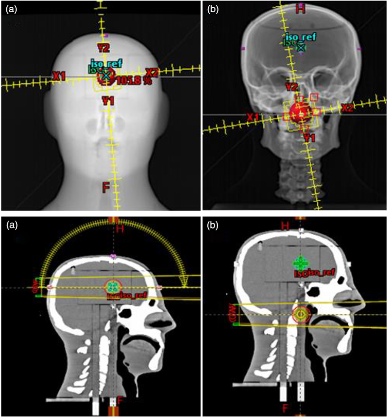
Figure 1. VMAT treatment plans for (a) the target located in the brain using one and half arcs and (b) the target located in the neck (close to the trachea) using 2 full arcs. This figure presents the target size of 3 cm in diameter in the stereotactic end-to-end verification (STEEV) head phantom.
Results
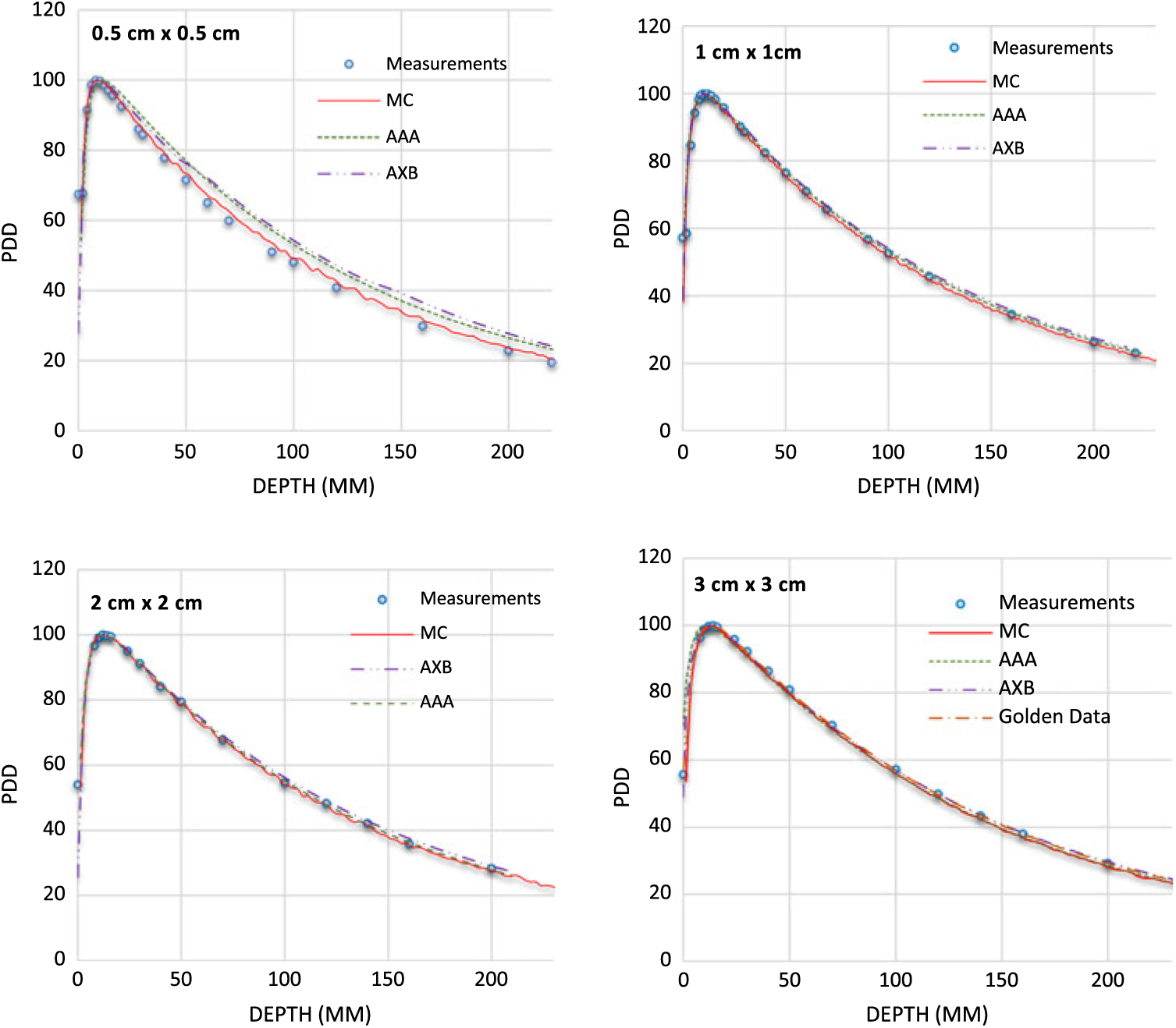
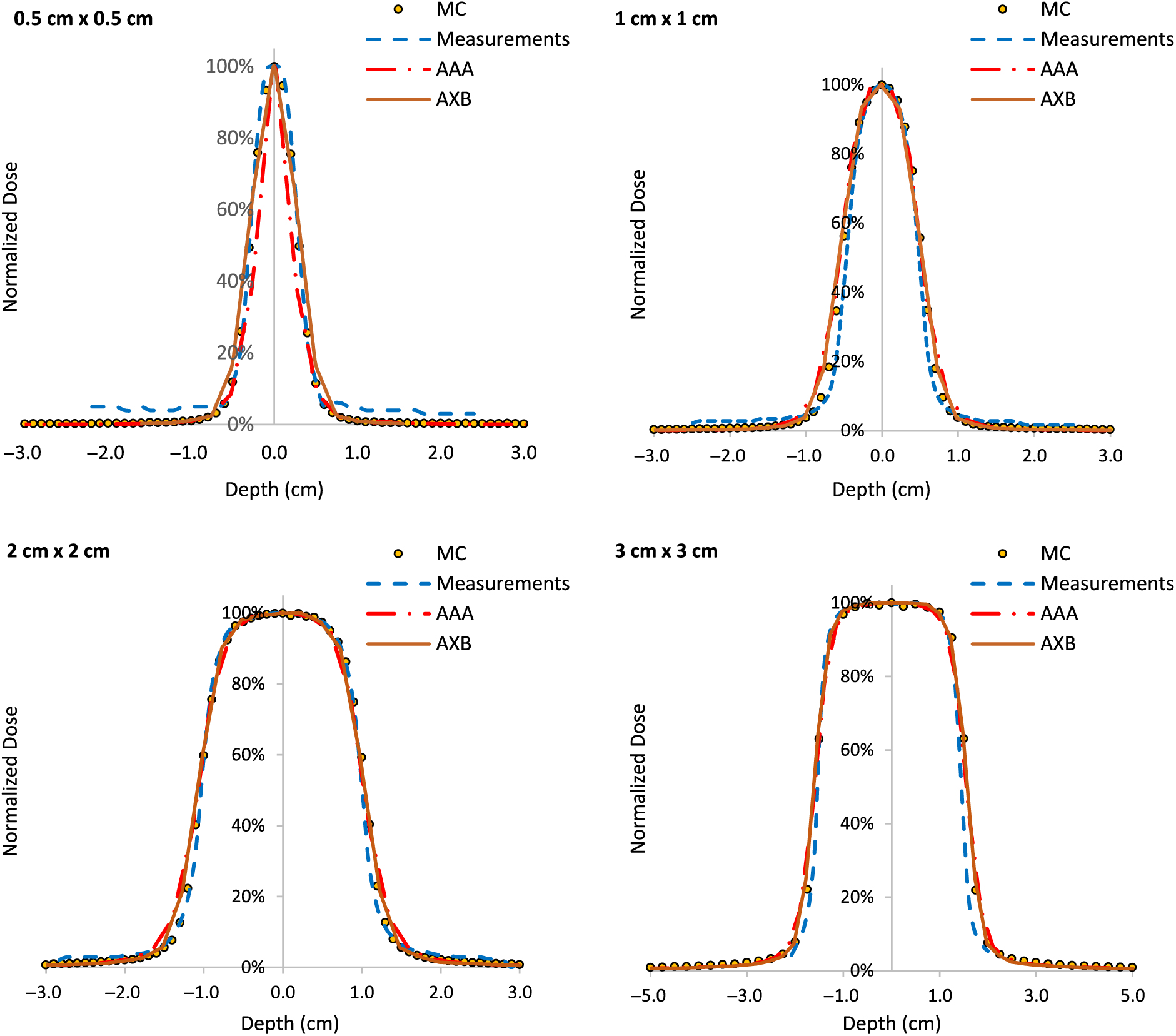
PDDs for 0·5 × 0·5 cm2, 1 × 1 cm2, 2 × 2 cm2 and 3 × 3 cm2 field sizes and for 6 MV, 6FFF MV, 10 MV and 10FFF MV photon beam energies are shown in Figures 2–5. The Varian GBD for a 3 × 3 cm2 field size is also shown in Figures 2–5. Figures 6 and 7 show beam profiles measured for 6 MV and 6FFF MV photon beams respectively at a depth of 5 cm comparing MC simulation, measurements and the AAA and AXB calculation algorithms. For the 6 MV photon, the FWHM values derived from MC, W1 Exradin measurements, AAA and AXB profiles are 0·61, 0·51, 0·64 and 0·64 cm for the 0·5 × 0·5 cm2 field size; 1·01, 0·97, 1·15 and 1·15 cm for the 1 × 1 cm2 field size; 2·1, 2, 2·06 and 2·06 cm for the 2 × 2 cm2 field size; and 3·12, 3·0, 3·12 and 3·12 cm for the 3 × 3 cm2 field size, respectively. Similarly, for the 6FFF MV photon, the FWHM values derived from MC, W1 Exradin measurements, AAA and AXB profiles are 0·60, 0·60, 0·44 and 0·68 cm for the 0·5 × 0·5 cm2 field size; 1·08, 1·01, 0·85 and 1·10 cm for the 1 × 1 cm2 field size; 2·1, 2, 2·1 and 2·11 cm for the 2 × 2 cm2 field size; and 3·02, 3·0, 3·04 and 3·16 cm for the 3 × 3 cm2 field size, respectively.
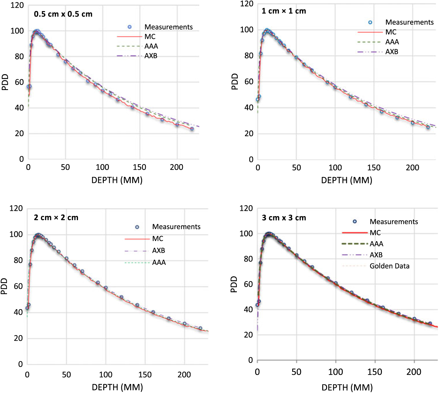
Figure 2. Percentage depth dose (PDD) profiles for 6 MV photon beams with field sizes ranging from 0·5 cm × 0·5 cm to 3 cm × 3 cm in a homogeneous water phantom comparing W1 Exradin scintillator measurements, Monte Carlo (MC) simulations and the calculation algorithms analytical anisotropic algorithm (AAA) and Acuros XB (AXB) in the eclipse treatment planning system. The Varian golden beam data are also included in the plot for a 3 cm × 3 cm field size.

Figure 3. Percentage depth dose (PDD) profiles for 6 FFF MV photon beams with field sizes ranging from 0·5 cm × 0·5 cm to 3 cm × 3 cm in a homogeneous water phantom comparing W1 Exradin scintillator measurements, Monte Carlo (MC) simulations and the calculation algorithms analytical anisotropic algorithm (AAA) and Acuros XB (AXB) in the eclipse treatment planning system. The Varian golden beam data are also included in the plot for a 3 cm × 3 cm field size.
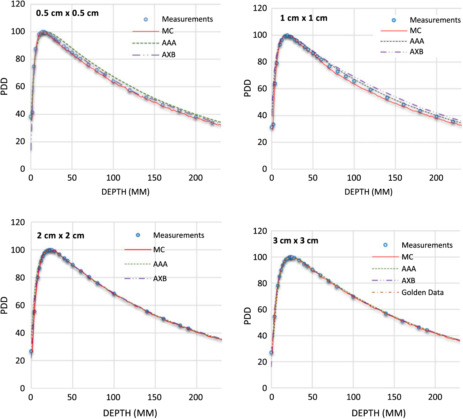
Figure 4. Percentage depth dose (PDD) profiles for 10 MV photon beams with field sizes ranging from 0·5 cm × 0·5 cm to 3 cm × 3 cm in a homogeneous water phantom comparing W1 Exradin scintillator measurements, Monte Carlo (MC) simulations and the calculation algorithms analytical anisotropic algorithm (AAA) and Acuros XB (AXB) in the eclipse treatment planning system. The Varian golden beam data are also included in the plot for a 3 cm × 3 cm field size.

Figure 5. Percentage depth dose (PDD) profiles for 10 FFF MV photon beams with field sizes ranging from 0·5 cm × 0·5 cm to 3 cm × 3 cm in a homogeneous water phantom comparing W1 Exradin scintillator measurements, Monte Carlo (MC) simulations and the calculation algorithms analytical anisotropic algorithm (AAA) and Acuros XB (AXB) in the eclipse treatment planning system. The Varian golden beam data are also included in the plot for a 3 cm × 3 cm field size.

Figure 6. Beam profiles for 6 MV photon beam with field sizes ranging from 0·5 cm × 0·5 cm to 3 cm × 3 cm in a homogeneous water phantom comparing W1 Exradin scintillator measurements, the calculation algorithms analytical anisotropic algorithm (AAA) and Acuros XB (AXB) in the eclipse treatment planning system and Monte Carlo (MC) simulated data.
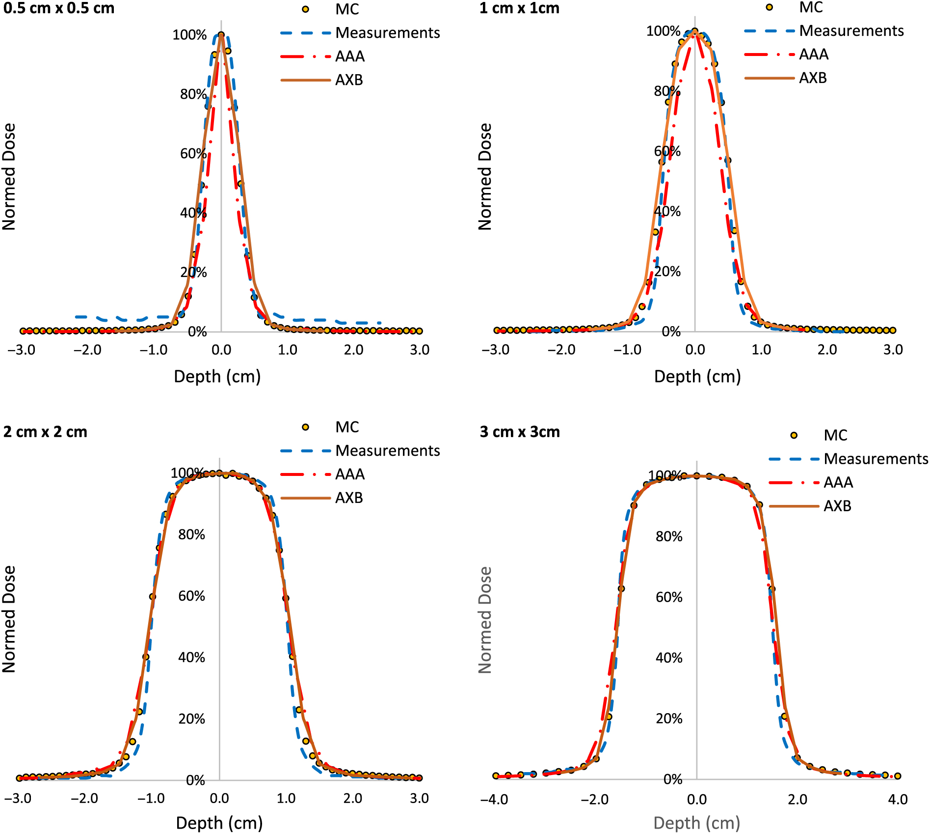
Figure 7. Beam profiles for 6FFF MV photon beam with field sizes ranging from 0·5 cm × 0·5 cm to 3 cm × 3 cm in a homogeneous water phantom comparing W1 Exradin scintillator measurements, the calculation algorithms analytical anisotropic algorithm (AAA) and Acuros XB (AXB) in the eclipse treatment planning system and Monte Carlo (MC) simulated data.
Table 1 shows the PDD results at depths of 5, 10 and 20 cm comparing MC simulated data, measured data with the W1 Exradin detector and calculated data from the eclipse TPS with both AAA and AXB calculation algorithms. The data show good agreement between the W1 Exradin measurements and the MC simulation data. Data in Table 1 show that the difference of the PDDs between AAA and measurements averaged over all the energies is 6·6, 1·7, 0·7 and 1·2 at the depth of 5 cm; 4·4, 2·0, 1·2 and 1·2 at the depth of 10 cm; and 5·5, 2·5, 0·5 and 1·2 at the depth of 20 cm for field sizes of 0·5 × 0·5 cm2, 1 × 1 cm2, 2 × 2 cm2 and 3 × 3 cm2, respectively. Similarly, the difference between AXB and measurements averaged over all beam energies is calculated to be 4·6, 0·2, 1·6 and 1·9 at the depth of 5 cm; 3·2, 1·6, 2·8 and 2·1 at the depth of 10 cm; and 8·2, 4·8, 4·1 and 3·3 at the depth of 20 cm for field sizes of 0·5 × 0·5 cm2, 1 × 1 cm2, 2 × 2 cm2 and 3 × 3 cm2, respectively. ROFs from measurements and TPS calculations using AAA and AXB are tabulated in Table 2 for different beam energies and field sizes. Compared with the W1 Exradin measurements, the ROF values are underestimated by the AAA algorithm, averaged over all the energies by 9·9, 2·4, 1·4 and 0·7% for field sizes of 0·5 × 0·5 cm2, 1 × 1 cm2, 2 × 2 cm2 and 3 × 3 cm2, respectively. Similarly, the ROF values are overestimated by the AXB algorithm, averaged over all the energies by 1·3 and 1·6% for 0·5 × 0·5 cm2 and 1 × 1 cm2 field sizes and underestimated by 0·3 and 0·9% for 2 × 2 cm2 and 3 × 3 cm2 field sizes, respectively. In general, the AXB algorithm is in good agreement with measurements for small fields than the AAA algorithm.
Table 1. Percentage depth dose values acquired at different depths comparing Monte Carlo simulated data, measured data with the W1 Exradin detector and calculated data from the eclipse TPS with both the analytical anisotropic algorithm (AAA) and Acuros XB (AXB) calculation algorithms for different field sizes and photon beam energies
Table 2. Relative output factors (ROFs) comparing calculated data using both analytical anisotropic algorithm (AAA) and Acuros XB (AXB) algorithms against measurements using the W1 Exradin detector. %diff is calculated for eclipse AAA and AXB with respect to W1 Exradin scintillator measurement
Table 3 shows the comparison of isocenter point doses for MC simulation, W1 Exradin measurement and AAA and AXB TPS calculation algorithms at the centre of different brain target sizes in the STEEV phantom (Figure 1a). The target sizes ranged from 0·5 to 3 cm3. For the 0·5 cm3 target size, results from the MC simulation, doses calculated by Eclipse AAA and AXB algorithms are about 1·5, 4·3 and 1·3% higher than dose measured by W1 Exradin, respectively. For the 1 cm3 target size, doses simulated by MC and calculated by Eclipse AAA and AXB algorithms are 3·3, 2·7 and 4·5% higher than that measured by W1 Exradin, respectively. For the 2 cm3 target, MC simulation, AAA and AXB show dose difference of −2·2, 4·0 and 3·4%, respectively, compared to W1 Exradin measurements, and similarly, for the 3 cm3 target the MC simulation, AAA and AXB show dose difference of −1·8, 2·1 and 1·6%, respectively, compared to measurements. Table 4 shows the point doses at the centre of the target located at the neck region close to the trachea (Figure 4b) using MC simulation, W1 Exradin measurements and AAA and AXB TPS calculated dose. For the 0·5 cm3 target size, the dose simulated by MC and calculated by TPS AAA and AXB are about 0·9, 4·3 and −1·9% different from measurements, respectively. For the 1 cm3 target size, doses simulated by MC and calculated by Eclipse AAA and AXB algorithms vary by about −4·6, 5·6 and 5·1% compared to measurements, respectively. For the 2 cm3 target, MC simulation, AAA and AXB show dose differences of 4·9, 6·5 and 5·4%, respectively, compared to measurements and similarly for the 3 cm3 target, the MC simulation, AAA and AXB show dose differences of 4·9, 6·5 and 5·4%, respectively, compared to measurements. In general, the MC simulation and AXB show good agreement with measurement for small fields’ measurements in the anthropomorphic head phantom.
Table 3. Comparison of isocenter point doses for MC simulation, W1 Exradin measurement and the analytical anisotropic algorithm (AAA) and Acuros XB (AXB) TPS calculation algorithms at the centre of different brain target sizes of the anthropomorphic head and neck phantom. The beam energy used for the treatment planning and delivery is 10FFF MV
* The differences (%diff) were found with W1 Exradin measurements.
Table 4. Comparison of isocenter point doses for MC simulation, W1 Exradin measurement and the analytical anisotropic algorithm (AAA) and Acuros XB (AXB) TPS calculation algorithms at the centre of different neck target (close to trachea) sizes of the anthropomorphic head and neck phantom. The beam energy used for the treatment planning and delivery is 6 MV
* The differences (%diff) were found with W1 Exradin measurements.
Discussions
In modern radiation therapy, recent technological advances in dose delivery, patients positioning, target localisation and immobilisation of patients have led to more complex treatment planning such as SRS and SBRT. In these techniques, small field sizes are often used to treat small target volumes and minimising doses to surrounding normal tissues. Consequently, it becomes necessary to be able to determine the dose in small photon beams with high accuracy, both in TPS commissioning and patient-specific quality assurance. However, the lateral electron disequilibrium, the finite size of the detectors and the non-water equivalence of the materials make the accuracy of small-field dosimetry challenging. Many publications have been concerned with the validation and comparison of the AXB algorithm against measurements, MC simulations, AAA algorithms or a combination of these modalities in small fields.Reference Zhen, Hrycushko and Lee47–Reference Fogliata, Lobefalo and Reggiori49 Stathakis et al.Reference Stathakis, Esquivel and Quino31 investigated the accuracy of small field dosimetry using the AXB dose calculation algorithm in homogenous and heterogenous media. They concluded that in a homogeneous phantom, the AAA and AXB showed good agreement with MC simulations. However, when dose calculations in heterogenous phantoms were compared to MC simulations, the AXB had better agreement than AAA. Qin et al.Reference Qin, Gardner and Kim33 evaluated plastic scintillator dose measurements for small field stereotactic patient-specific quality assurance. They concluded that the Exradin detector demonstrated superior performances in plans with small fields and heavy modulation, and thus the Exradin is a suitable detector for clinical routine SRS quality assurance dose measurements. Fogliata et al.Reference Fogliata, Lobefalo and Reggiori49 evaluated the dose calculation accuracy for small fields defined by jaws or MLCs using the AAA and AXB algorithms. They used single point output factor measurement using a PTW microDiamond detector for 6 MV, 6FFF MV and 10FFF MV beams with a Varian TrueBeam. Measurements were compared with the AAA and AXB dose calculation algorithms. They found an agreement of less than 0·5% for field sizes as small as 2 × 2 cm2. For smaller fields, both algorithms either overestimated the dose for jaw-defined field sizes or underestimated the dose for MLC-defined field sizes. In the very small field region (as small as 0·5 × 0·5 cm2), the AXB achieved agreement within 3% with measurements. In this study, we observed that the AXB showed good agreement of about 0·3% with Exradin measurements, whereas the AAA showed a relative difference of 2·9% (Table 2). The AAA algorithm shows dose underestimation of about 10·9% for field sizes as small as 0·5 × 0·5 cm2 with the 10 MV beam. The AXB algorithm shows dose underestimation of less than 1% for 2 × 2 cm2 and 3 × 3 cm2 field sizes and dose overestimation of less than 2·5% for 0·5 × 0·5 cm2 and 1 × 1 cm2 field sizes (Table 2).
Godson et al.Reference Godson, Ravikumar and Sathiyan34 investigated the depth of dose maximum (Dmax) and depth dose at 10 cm (DD10) with different detectors including cylindrical ion chamber, shielded diode, unshielded diode and parallel plate ion chamber. They used small field sizes of 1 × 1 cm2, 2 × 2 cm2 and 3 × 3 cm2 using a Varian linear accelerator with 6 MV photon beam. They reported the biggest detector-to-detector variation for DD10 for the 1 × 1 cm2 and negligible deviation was found for larger fields. For 1 × 1 cm2 field size, they reported DD10 minimum and maximum values of about 57% (using shielded diode) and 60% (using parallel plate ion chamber), respectively. In this study, we measured DD10 of 55·9% for 6 MV photon beam and 1 × 1 cm2 field size, which agrees well with the shielded diode measurement. Also, the DD10 with shielded diode measurement by Gordon et al.Reference Godson, Ravikumar and Sathiyan34 of 59 and 61% for the field sizes of 2 × 2 cm2 and 3 × 3 cm2, respectively, agrees well with the W1 Exradin measurement of DD10 of 59·3 and 60·8% in our study. Pasquino et al.Reference Pasquino, Cutaia and Radici35 investigated dosimetric characterisation in small X-ray fields using a microchamber and a plastic scintillator detector. They measured PDDs for 1 × 1 cm2, 2 × 2 cm2 and 3 × 3 cm2 field size for 6 MV photon beam and acquired DD% at depths 5 cm, 10 cm and 20 cm. They concluded that both micro-ion chamber (A26 IC) and W1 Exradin could play an important role in small field relative dosimetry. Our measurements for 6 MV photon beam agreed well with their results. AAA and AXB beam profile and PDD results were not very different in a homogeneous medium. However, in the presence of heterogeneity, our results confirmed that AXB presents closer agreement with measured values compared to AAA (Tables 3 and 4). The results in Tables 3 and 4 showed that the average dose difference between measurements and MC simulation is 0·2 and 3·8% for the tumours located in the brain and neck region, respectively.
There are some limitations that may be associated with the measurements, simulations and TPS calculations when dealing with small fields such as the accurate positioning of the detector for measurement, accurate material composition for AXB algorithm and noise in MC simulations for small voxel size. Although we attempted to position the detector at the centre of the tumours and also aligned the detector correctly to the field centre for accurate measurements of PDDs, profiles and ROFs, determining the exact detector positioning in the centre of the field is still a challenge. Also since the AXB algorithm uses the material composition for the voxels from a predefined material library for dose calculations, accurate material composition data for each voxel are important for accurate dosimetry.
Conclusions
We have investigated the accuracy of AXB algorithm and the AAA in small fields against W1 Exradin and MC techniques. We made the comparison of dosimetric parameters including PDDs, beam profile and ROFs in water phantom. We observed that the W1 Exradin measurements agree well with MC simulation in both homogeneous medium and heterogeneous anthropomorphic phantom medium representing a patient. Therefore, W1 Exradin can be used efficiently to measure dosimetric parameters in small fields and for patient-specific quality assurance measurements. In both homogenous and heterogeneous media, the AXB algorithm dose prediction agrees well with both measurements and MC simulation and was found to be superior to the AAA algorithm.
Author ORCIDs
Ernest Osei 0000-0002-4114-3273
Acknowledgements
The author Sepideh Behinaein would like to acknowledge with gratitude the support received from all the Medical Physicists, Electronic Technologists, Medical Physics Associate, Radiation Therapists and Radiation Oncologists in the Radiation Oncology Program at the Grand River Regional Cancer Centre during the time of residency at the Medical Physics Department.