INTRODUCTION
Monte Carlo method has proven to be the most accurate calculation algorithm for assessing the dose distribution in radiotherapy.Reference Toossi, Momennezhad and Hashemi 1 The beam characteristics are often different due to variation in accelerator designs and on-site beam tuning. It is necessary to simulate each accelerator individually to calculate the phase space data. Monte Carlo simulation is usually used as a benchmarking tool in predicting dose distributions in phantoms,Reference Serrano, Hachem and Franchisseu 2 especially in cases where the experimental dose measurement is very difficult, or reaches its limitations.
The usual approach in the evaluation of the accuracy of dose calculation algorithms is to compare results with experimental measurements The purpose of this research is comparison between 6 MV Primus (Siemens, Munich, Germany) LINAC simulation output with commissioning data using EGSnrc.
In this work, the EGSnrc MC code, including user codes BEAMnrc and DOSXYZnrc, was employed to model a Siemens Primus linac working in 6 MV photon mode and to calculate the dose distributions in a water phantom and also measure the percentage depth dose (PDD) and beam profile in the model. The data were compared with that calculated using treatment planning system computer measured in water.
MATERIAL AND METHODS
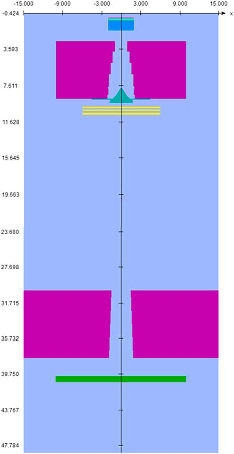
In this study, Monte Carlo simulation was carried out using BEAMnrc and DOSXYZnrc codes to perform all dose calculation in this project. Both programs are based on an electron gamma shower user code (EGSnrc) that come as a package under licence to the National Research Council of Canada (nrc). According to manufacturer’s specifications about the geometry and the materials, the MC model of the treatment head of the 6 MV Primus (Siemens) linac Systems, was built using the following component modules: the exit window, target, primary collimator, flattening filter, monitor chamber and secondary collimator. The Primus accelerator simulation components are shown in Figure 1.

Figure 1 Simulated head of linear accelerator.
PEGS4 (EGS preprocessor) cross-section data for the specific materials in the accelerator were from 700icru PEGS4data file. This data file contains cross-section data for particles with kinetic energy as low as 0·01 MV and physical density such as mass density, atomic number, and electron density for all the different materials used in the accelerator.
A total of 2×10⁸ histories were run in the accelerator head calculations. The electron cut-off energy (ECUT) was set to 0·7 MeV while the photon cut-off energy (PCUT) was set to 0·01 MeV.
The primary output of the BEAMnrc simulation for the head of linear accelerator is a file called phase space file which has information about all the particles leaving the accelerator. This phase space was scored in a plane upright to the beam axis at 100 cm distance from the target. The BEAMDP program (BEAM utility program) was used to read and process the data in the phase space files to plot energy spectrum of photon beam in four fields (Figure 2).
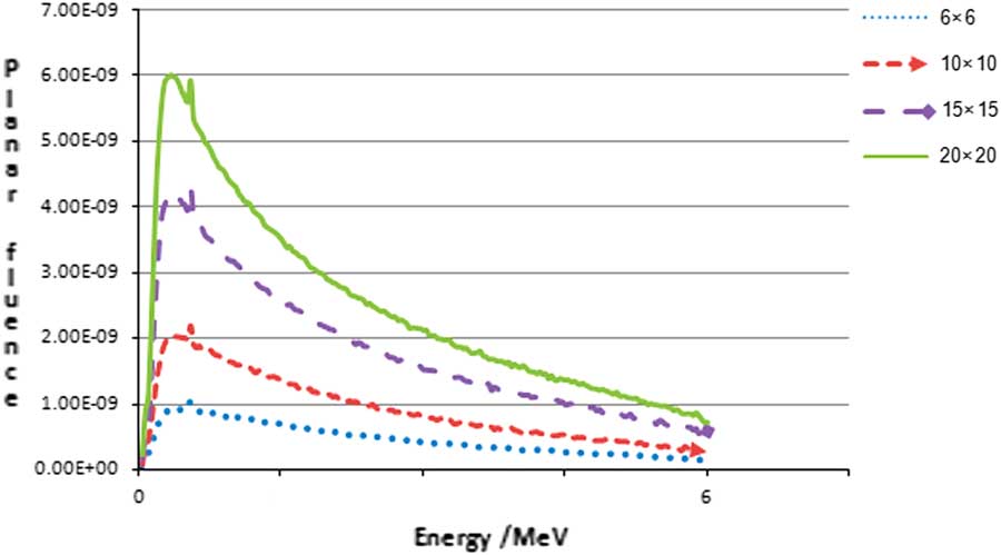
Figure 2 Energy spectrum of photon beam in four fields with BEAMDP.
To validate the Monte Carlo model for the photon beam output from the Primus linear accelerator, five phase space files were created with 4×4 cm2, 6×6 cm2, 10×10 cm2, 15×15 cm2, 20×20 cm2 field sizes. These files can be used as input file to DOSXYZnrc simulation to determine the dose distribution in water phantom created by DOSXYZnrc program. The water phantom was created using DOSXYZnrc code distribution. The voxel size used was 0·5×0·5×0·2 cm3. The water phantom was located at source to surface distance (SSD) of 100 cm. The electron cut-off energy (ECUT) was set to 0·7 MeV, the photon cut-off energy (PCUT) was set to 0·01 MV. A total of 1×10⁹ histories were run in the phantom simulation, the statistical uncertainty of the simulation was kept <1%.The output file from DOSXYZnrc program (*.egslst) was analysed by Microsoft Office Excel. Dose results were analysed by producing the percentage depth dose (in five fields) in the central axis and dose profiles (in three fields) (Figures 3 and 4).

Figure 3 The percentage depth dose of calculated Monte Carlo (MC) and measurement of commissioning results in 5 field sizes.

Figure 4 Beam profile comparison of commissioning data and calculated Monte Carlo (MC) results at 10 cm depth.
The PDD and beam profile were normalised to the maximum dose at depth 1·5 cm. The simulated PDD and beam profile were compared with that calculated using commissioning data.
Output factors have been determined by dividing the dose in a reference point for a given field size by the dose in the same point for the 10×10 cm2 reference field for the same amount of incident radiation on the X-ray target. For the total scatter output factor Sc,p, these dose points were taken from the total dose distribution calculated in the full scatter phantom, the values for the collimator scatter output factor Sc were calculated in the air (by eliminating phantom in DOSXYZnrc). Once these two output factors are known, the phantom scatter output factor Sp is given through:
 $${\rm S}_{{\rm p}} \left( r \right){\equals}{\rm S}_{{{\rm c},{\rm p}}} \left( r \right)\,/\,{\rm S}_{{\rm c}} \left( r \right)$$
where Sc,p(r) is the total scatter factor defined as the dose rate (or dose per MU) at a reference depth for a given field size r divided by the dose rate at the same point and depth for the reference field (e.g., 10×10 cm2). Thus, Sc,p (r) contains both the collimator and phantom scatter and when divided by Sc(r) yields Sp(r).Reference Khan and Gibbons 3
Table 1 shows the final values of Sp at depth 10 cm for the five field sizes. The parameter TPR20,10 is defined as the ratio of doses on the beam central axis at depths of 20 cm and 10 cm in water obtained with a constant source to detector distance of 100 cm and a field size of 10×10 cm2 at the position of the detector. The TPR20,10 can be related to the measured PDD20,10 using the following relationshipReference Podgorsak 4 , 5 :
 $${\rm TPR}_{{20,10}} {\equals}1 \! \cdot \! 2661\,{\rm PDD}_{{20,10}} -0 \! \cdot \! 0595$$
Table 1 Table of Sp at depth 10 cm for the five field sizes

Values for TPR20,10 were calculated for five field sizes. The TPR20,10 values for depth 10 cm and fields size 10×10 cm2 are presented in Table 2.
Table 2 Table of PDD20,10 and TPR20,10 (depth=10 cm, field size 10×10 cm2)

TMR is a special case of TPR and defined as the ratio of the dose rate at a given point in phantom to the dose rate at the same source-point distance and at the reference depth of maximum dose. The TMR at depth 10 cm is calculated from PDD using the following relationshipReference Podgorsak 4 , 5 :
 $$\eqalignno{& {\rm TMR}_{{(z,{\rm A},{\rm hv})}} \cr & {\equals} \left( {{\rm PDD}_{{(z,{\rm A},{\rm hv})}} /100} \right)\left( {f{\plus}z / f{\plus}z_{{\max }} } \right)^{2} $$
where PDD is the percentage depth dose, z is the depth, z max is the reference depth of maximum dose , f=SSD. The PDD depends on four parameters: depth in a phantom z, field size A, SSD (often designated with f) and photon beam energy hv.
The TMRs values for depth 10 cm and fields size 10×10 cm2 are presented in Table 3.
Table 3 Table of Tissue-maximum ratio values for depth 10 cm (SSD=100 cm)

RESULTS AND DISCUSSION
Measurements of PDD
To validate the photon production of the modelled primus LINAC, the photon spectrum and dose distribution were calculated using Monte Carlo simulation.
The photon energy spectrum as a function of photon energy is shown in Figure 2. The spectrum was plotted at the phantom surface (SSD=100 cm) for the four field size. Then the simulated PDD for the five field sizes were compared with that calculated using commissioning data as shown in Figure 3.
Comparison showed a good agreement between simulated and calculated data at build-up region with a similarity in the shape of the curves. But an obvious difference at the surface region of both curves may be ascribed to electron contamination in the photon beam that interacts at the surface region of the simulated water phantom.Reference Pena, Franco and Gomez 6 This leads to difficulty to predict the actual value of deposited dose at the surface region. The simulated and calculated data for the depths D max agreed well, within 1·1% difference. Our results were in agreement with Aljamal and Zakaria’s result.Reference Aljamal and Zakaria 7
Measurements of profile
At 10 cm depth, the beam profiles determined by MC simulation and commissioning data. The simulated beam profile matched acceptable with that calculated at the central region (Figure 4).
The profile illustrates the discrepancy between the calculated results and the measured results. It can be caused by the uncertain setup of the ionisation chamber, leveling of the ionisation chamber, water tank, imprecise modelling of the linac head and random error that resulted during the simulation.Reference Jabbari, Sberi, Tvakoli and Amouheydari 8 In some condition for better results, we used voxel with various sizes, for example in the build-up region voxels was so smaller than voxels in the tail region.
These decrease the time of simulation and can perform better comparison between the results. Such calculates require high precision which can be achieved by increasing the number of histories of the simulation.Reference Stathakis, Balbi, Chronopoulos and Papanikolaou 9
Measurements of Sp
Sp calculated from Scp and Sc measurements using the relationship Equation (1). Table 4 shows the values of Sp at SSD=100 cm and depth 10 cm in five field sizes.
Table 4 The values of Sp (SSD=100 cm, depth=10 cm)

Sp values for fields ≥4 cm width are independent of beam defining system and dependent only on measurement depth, beam quality and beam area irradiated.Reference McKerracher and Thwaites 10 Average differences for five field sizes in this approach is about 0·83%.
Measurements of TPR20,10
In this study, the TPR values calculated from PDD using the relationship Equation (2). This empirical relationship was obtained from a sample of almost 700 linacs.Reference Chang, Wei Wang and Shiau 11 Good agreement was found between calculated.
TPR20,10 using Monte Carlo simulation and commissioning data. The difference between Monte Carlo simulation and commissioning data is about 0·29% in SSD=100 cm and Depth=10 cm.
Measurements of TMR
At depths 10 cm, the TMRs calculated from PDD data using the relationship Equation (3) in five field sizes.The difference in the TMRs values between Monte Carlo simulation and commissioning data in five fields, represented in Table 5.
Table 5 The difference in the TMRs (SSD=100 cm, depth=10 cm)

Good agreement in field sizes ≤10 cm2 (about 0·6–1%) and acceptable agreement in field sizes ≥10 cm2 (about 2·5%) was found between calculated TMRs using Monte Carlo simulation and commissioning data. The decrease in TMR with field size is due to; incident scattered radiation, changing balance with depth of phantom scatter and the presence of secondary electrons from the beam.( contaminated electrons).Reference Toutaoui, Ait chikh, Khelassi-Toutaoui and Hattali 12
CONCLUSIONS
In this study, the PDD, beam profile, Sp, TPR20,10 and TMR were calculated using Monte Carlo simulation and compared with the measurement performed by commissioning data. To obtain accurate results from Monte Carlo simulations in radiotherapy calculations, precise modelling of the linac head and a sufficiently large number of particles are required.Reference Ding 13 , Reference Verhaegen and Seuntjens 14
The results of the beam quality specification comparison were more consistent, with this study method to calculate TPR20,10 values agree about 0·29%.
Data in Table 2 suggest that they can be used to provide a close approximation (within 0·2%, for the beam evaluated in this study) to TPR20,10 from PDD data, if direct measurement from TPR data is unavailable.
The results showed that the BEAMnrc and DOSXYZnrc codes have an excellent performance in calculating the depth dose, beam profile, TPR20,10 and TMR measurements for 6 MV photon beam. The Monte Carlo model of primus 6 MV linear accelerator built in this study can be used as promising method to calculate the dose distribution for cancer patients.
Acknowledgements
The authors would like to thank Mr H. Babapour for his kind cooperation. The manager and staff of Shahid Rajaei hospital of Babolsar are also greatly appreciated for their efficient support regarding this study.
Ethical Standards
This article does not contain any studies with human participants or animals performed by any of the authors.