
The Social Security Administration (SSA) oversees the provision of benefits across a range of programmes serving the elderly, the poor, the disabled, widows and dependent children. The most familiar programme, pensions for elderly or the Old-Age (OA) component of the Social Security programme, is applicant-driven and formula-based. At retirement, eligible workers apply for benefits and a standard formula – based on long-term earnings history – determines benefits. These programme features imply a fairly high level of uniformity and equity across states. However, this simple implication is not realised in practice. The level of benefits flowing to states varies, predictably, depending on the proportion of seniors in the state population, but also, surprisingly, varies even accounting for that factor. In the state of Michigan, the total amount of OA benefits paid to state residents in 2010 was $18.2 billion or $13,400 for each person in the state aged 65 or older. This is in contrast to the state of Louisiana, where the total amount of OA benefits paid to state residents in the same year was $5.4 billion or $9,700 for each person in the state aged 65 or older. This is an extraordinary difference, and these types of differences in aggregate benefit levels across states have profound redistributive implications given the size of the programme relative to the total economy. What explains this disparity? To address this question, the article proceeds in three parts. First, we briefly summarise a diverse set of literature that describes and explains differences in federal spending in the states. Second, we describe the size and operation of the OA programme, and differentiate between the scope of OA coverage and average benefit payments. In this section, we develop several specific hypotheses about why expenditures may vary across states. Third, we present a statistical model that identifies the key drivers of cross-state variation in OA coverage and benefits. We ultimately find that state unemployment rates are strongly linked to OA expenditures – in states where unemployment is high, we observe broader coverage and higher benefits. This surprising result highlights the multiple policy goals that the OA programme serves – both lifting seniors out of poverty and shifting federal resources to states experiencing high levels of unemployment.
How do policy outcomes – and federal spending – vary across the states?
Research on state-to-state differences in public policy outcomes takes three broad forms: work that emphasises features of states, work that emphasises the actions of national elected official and bureaucrats and work that reveals how state actors can influence the flow of resources from the federal government. The state-centred work analyses differences related to state-level public policy choices directly under the control of state legislatures and governors. State-level variation has been linked to diverging paths of historical development, diverse political cultures, the presence of different racial and ethnic majorities, the ideologies of political leaders and citizens, different types of dominant economics interests and elites, and the economic health of the state (Elazar Reference Engelhardt and Gruber1966; Jacoby and Schneider Reference Jacoby and Schneider2001; Amberg Reference Amberg2008; Lieske Reference Lieske2010). The variety of policies that this research encompasses is quite broad: from income support programmes and Medicaid to child support enforcement actions (for the latter, see Keiser and Soss Reference Keiser and Soss1998). States also react in important ways to the policy choices of neighbouring states (Peterson and Rom Reference Peterson and Rom1990). The DC-centred work analyses how federal choices – in the White House, Congress or federal administrative agencies – may concentrate spending in particular states. Berry et al. (Reference Berry, Burden and Howell2010) examine the geographic distribution of federal spending (direct expenditures and grants) focussing on how spending varies across congressional districts and counties. They find that districts with a more senior representative from the president’s party tend to see higher federal expenditures of this form. In work designed to determine how much federal spending in various forms translates into economic activity, Nakamura and Steinsson (Reference Nakamura and Steinsson2014) demonstrate that federal spending – specifically, military procurement – can vary and have quite different impacts across states and regions. A third set of work investigates how state-level actions impact the level of federally administered programme spending (Rich Reference Rich1989; Nugent Reference Nugent2009). States can, for example, invest resources to assist eligible residents in applying for a variety of benefits that are fully or partially funded by the federal government – supplemental nutrition assistance, unemployment insurance, Medicaid and even veteran’s disability benefits (Miller and Kaiser Reference Miller and Kaiser2012). States can also vary in the way administrative determinations make it easier or harder to qualify for federal assistance: the SSA has identified substantial state-to-state variation in the rejection of initial disability claims (Strand Reference Strand2002) and the Department of Agriculture has documented state variation in Temporary Assistance for Needy Families payments – which impacts eligibility for, and amount of, supplemental nutrition assistance (Hanson and Andrews Reference Hanson and Andrews2009).
The aggregate effect of these federal and state choices generates quite remarkable differences in the “return” on tax dollars across states. The ratio of fiscal year 2013 federal spending to gross revenue collections for the entire United States was about $1.10 (Internal Revenue Service 2014; Pew Reference Pew2014). The expenditure total excludes interest payments on federal debt, classified expenditures and international transactions, but remains above $1.00 as some of the spending is financed by borrowing. For some states, this ratio is over $3.00 (Mississippi, New Mexico and West Virginia), whereas other states are large net contributors to the fiscal union, with ratios below $0.75 (Minnesota, Delaware, New Jersey and Nebraska). This disparity – and the fact that Red States are more often net beneficiaries – has attracted attention from journalists and other observers (e.g. see Gilson Reference Gilson2012; Tierney Reference Tierney2014).
The federal OA programme may be unique in that none of the literature on state policy variation applies. Eligibility and benefit levels are strictly a function of federal rules – there is no state administrative discretion to alter benefit levels. There is also no federal agency discretion that could result in higher benefits in particular states. State or federal administrative actors, members of Congress, state governors or legislators cannot influence the average benefit for workers only in particular states. Early DC decisions can, and did, impact the scope of coverage and eligibility in ways that disadvantaged some states, particularly Southern states, but today nearly 95% of US workers are covered by the OA programme. The OA programme is interesting precisely as it operates outside the influence of state-level actors but accounts for a remarkably large proportion of the overall flow of federal expenditures to the states. It may be possible for states to attempt to lure seniors – and their Social Security checks – by offering low or no income taxes on benefits, but there are few other steps that state leaders could take to influence the level of benefits that flow to their state. The one exception is whether or not participants in the states’ public sector retirement plan are also covered by Social Security – in seven states all public sector workers participate in Social Security, and in 33 states no public sector workers participate. Federal legislative choices are also unlikely to result in cross-state differences. Members of Congress can change the way that the benefit levels are determined or adjusted upwards each year, but those choices apply to all recipients in the same way, regardless of place of residence.
Despite the absence of direct opportunities to influence the flow of resources to particular states, the state-to-state variation in OA programme outcomes remains important for two reasons. First, the sheer size of the programme suggests that even small state-to-state variation may be important. The combined benefit expenditures of the Old-Age and Survivors Insurance components of Social Security approached $700 billion in fiscal year 2014, nearly 20% of the entire federal budget. With the exception of Medicaid, the OA programme is much larger than the sum of all the various grant and transfer payments addressed in the literature on state-to-state variation in federal spending. Second, the literature on state variation highlights differences in the economy of the states – states have different dominant industries, levels of income and unemployment levels. These differently situated states could experience widely divergent policy outcomes even under a standardised approach to the calculation of benefits and eligibility. The link between particular state features and OA expenditure across states is poorly understood, at best.
What is the OA programme and how does it impact individual states?
In 2014, nearly 42 million Americans received Social Security OA benefits on a monthly basis – 39 million retirees, two million spouses and almost one million children (SSA 2015). As perhaps the most effective anti-poverty programme in the United States, the OA component lifted more than 14 million seniors out of poverty in 2011 (Van de Water and Sherman Reference Van de Water and Sherman2012). In fact, OA payments are largest source of retirement income for persons aged 65 and older [Government Accountability Office (GAO) 2012].
The OA programme is financed through employee and employer payroll taxes and provides cash retirement benefits to workers upon retirement at a designated age. Workers are eligible for OA benefits if they have a work history that includes Federal Insurance Contributions Act (FICA) withholdings over a period of roughly 10 years. OA benefits are then determined by a formula that includes 35 years of earnings history. The SSA computes an average monthly indexed wage – indexed to account for inflation – and calculates benefit based on that wage. Both benefits and FICA withholdings are capped. This combination of uniform eligibility requirements and formula-based benefits means that similarly situated workers will receive identical benefits independent of where they live. There is no adjustment of OA benefits based on place of residence. In addition, there is no link between OA benefits and receipt of other benefits or eligibility for other services. OA benefits are the same if a recipient lives at home or is a resident of a skilled care nursing facility. In addition, OA benefit levels do not vary depending on eligibility for, or participation in, Medicare or Medicaid. The most important exceptions to this uniform treatment of earnings are the Windfall Elimination Provision and the Government Pension Offset: OA benefits levels (for worker or survivor) are reduced if an individual worked for an employer who did not withhold Social Security taxes. Social Security benefits may also be reduced if individuals file for benefits before full retirement age and may be further reduced if benefits are claimed early and the recipients continue to earn income from work.
If individual benefits are strictly a function of earnings and there are no discretionary choices about eligibility or benefit levels, then the primary factor that should explain variation in OA expenditures is the proportion of the state population aged 65 or over. Figure 1 summarises the link between senior population and the level of benefits flowing to each of the 50 states – the relationship is obviously positive but also very noisy.
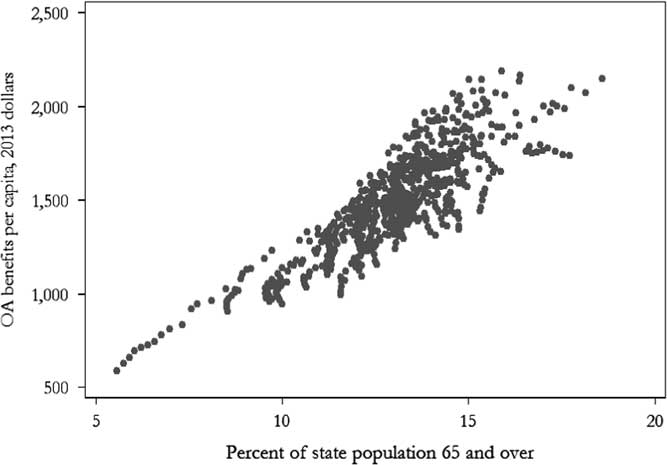
Figure 1 Total real Old-Age (OA) benefits per capita and state senior population, 1999–2013.
Different metrics tell a similar story. One convenient way to describe the impact of OA expenditures in individual states is to look at the ratio of OA expenditures to state gross domestic product (GDP). This metric is summarised, nationally and for Michigan and Louisiana, in Figure 2.
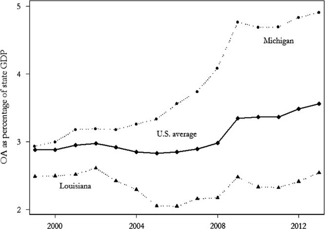
Figure 2 Old-Age (OA) programme expenditures as a percentage of state gross domestic product (GDP), 1999–2013.
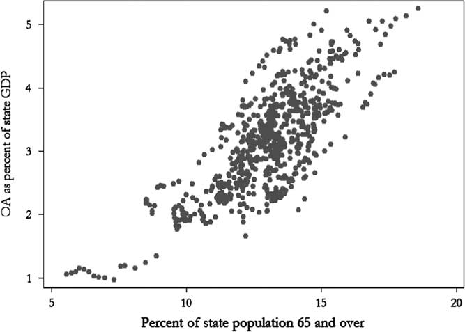
As suggested in the introduction, the OA programme has a much larger impact in Michigan than in the Louisiana – and this large difference is quite persistent over time. One obvious candidate reason for this difference is the size of the senior population in each state and, of course, this matters. Similar to Figure 1, Figure 3 summarises OA expenditures as a percentage of state GDP and the proportion of the state population over age 65 for each state from 1999 to 2013.

Figure 3 Old-Age (OA) expenditures as percentage of state gross domestic product (GDP) and state senior population, 1999–2013.
The figure demonstrates the link between the senior population and the economic importance of OA expenditures, but also highlights the tremendous variation in the impact of OA expenditures on the state economy in states with very similar senior populations – states with 12–14% of the population aged over 65 are observed with impacts from 2 to 4% of state GDP. Why is this important? As part of efforts to understand the impact of federal spending on the economy, a study by Romer and Romer (Reference Romer and Romer2014) is one of a handful of attempts to assess the macroeconomic impact of Social Security benefits. Their focus is on the aggregate impact of legislated changes in benefit levels (such as the Tax Reform Act of 1969) on consumption. They find a large effect of benefit increases – a one-to-one increase in consumer spending (a permanent 1% increase in benefits translates into an immediate 1% increase in consumption in the same month, an effect that persists for at least five months). The implication is clear: Social Security transfer payments translate into direct and immediate economic benefits. Consistent with this implication, state-level work on the impact of Social Security on poverty among the elderly indicates that the programme reduces the elderly poverty rate from 48 to 7% in Michigan, but from 50 to 15% in Louisiana. Despite the uniform features of the programme, the elderly poverty rate remains twice as high in Louisiana as in Michigan (Van de Water and Sherman Reference Van de Water and Sherman2012).
Why do outcomes vary across states?
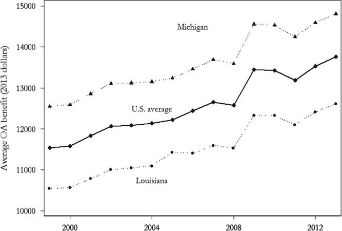
Across states that have similar over-65 populations, there are two factors specific to the OA programme that drive expenditures and account for most of the differences across states: variation in coverage (the proportion of the over-65 population receiving OA benefits) and variation in the average benefits (total OA payments divided by the number receiving benefits). Average benefits and coverage are summarised for the sample period in Figures 4 and 5.
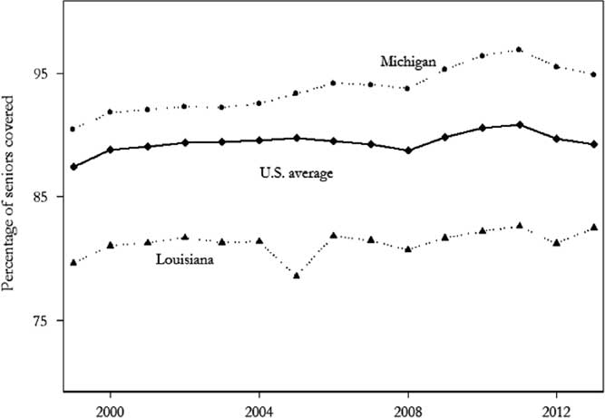
Figure 4 Percentage of population aged 65 and over receiving Old-Age (OA) benefits.

Figure 5 Average annual Old-Age (OA) benefit.
Michigan has a high and rapidly growing average benefit and a consistently high coverage relative to Louisiana – those persistent differences are the source of the discrepancy identified in the introduction.
But what explains these differences and why do they persist? We suggest two types of answers: state senior populations are not homogeneous and state economic performance varies.
Senior populations are not homogeneous (poverty, race, migration)
Senior populations are likely to be quite different across the states: some states have higher poverty rates, a growing senior population and high proportions of minority residents. We expect that each of these factors will be associated with the scope of coverage and the level of benefits.
What do we know about people who are covered in the OA programme? In a recent study of who never receives benefits under the OA programme, SSA researchers determined that seniors who were never beneficiaries fell into three categories: workers in noncovered positions, workers with insufficient work experience and late-arriving immigrants. Infrequent workers – who do not accumulate enough credits – account for about one-third of those not receiving benefits (Whitman et al. Reference Whitman, Reznik and Shoffner2011). These infrequent workers, unsurprisingly, tended to be poorer and have less education than workers who were eligible for benefits. Given these individual-level findings, we expect states with a workforce composed of people who are poor and poorly educated to have lower coverage.
Race may also matter. An inverse relationship between social welfare expenditures and the minority and/or black population has been found in a variety of work on the US states (Plotnick and Winters Reference Plotnick and Winters1985; Grogan Reference Grogan1994; Brown Reference Brown1995; Hero and Tolbert Reference Hero and Tolbert1996). Historically, the coverage of the Social Security OA programme varied widely across states – the initial exclusion of agricultural and domestic workers implied much lower coverage of the labour force in Southern states. This broad early exclusion implied that minority populations in the South – primarily African-Americans – would remain outside of the Social Security programme for decades, and the impact of this exclusion is still controversial (DeWitt Reference DeWitt2010). Although the OA programme has expanded to include 95% of the current workforce, the proportion of the covered senior population – the former workforce – is smaller, varies substantially across states and may impact both overall state coverage and average benefit levels.
Finally, state choices about whether state and local government workers will participate in Social Security should affect coverage rates. Until 1983, most state and local workers were also excluded and roughly one-fourth of all current state and local workers remain outside the programme (Whitman et al. Reference Whitman, Reznik and Shoffner2011). Some states exclude all state and local government workers; many states include all state and local government workers, and thus coverage in these states should be higher.
In addition to affecting coverage, state demographic characteristics should also influence average benefits. OA benefits are calculated based on a 35-year earnings history. In a state with many poor households, we would expect a lower average long-term earnings history than states with fewer poor households. A similar link should appear between education levels and average benefits. As highly educated workers have long-run lifetime earnings that are much higher than poorly educated workers, the average benefits should be higher in states with many highly educated workers. Finally, the senior populations will be much different in states that experience in-migration of seniors than in states that experience out-migration. Lin (Reference Lin1997) found that “leavers” – seniors who migrated – had higher levels of income and education than seniors who stayed in place after retirement. This leads us to expect that states experiencing larger increases in the number of seniors – states that are destinations for senior in-migration – should have higher coverage and higher benefits.
In sum, we expect that states with populations that are high proportion minority, with lower-than-average college completion rates, with fewer in-migrant seniors and with higher than average poverty rates, will have lower coverage and lower average benefit levels. States that have public sector pension plans that exclude workers from the OA programme will also have lower rates of coverage.
State economic experience is not homogeneous (current unemployment, prior wages)
States vary in both economic legacies (the structure of the state economy in terms of agriculture, manufacturing or service jobs) and in current economic performance. High levels of manufacturing employment, for instance, might be associated with historically higher levels of average wages. Further, labour markets can be highly regional, with high unemployment persisting in some regions even during booms or low unemployment persisting in other regions during recessions (the North Dakota energy boom in the recent recession, for instance). Recent economic research suggests that these differences are tied to both economic and demographic features of states and that the timing of business cycle peaks and troughs can be quite variable across states (Owyang et al. Reference Owyang, Piger and Wall2005).
State unemployment levels should affect coverage and benefits. States with low unemployment rates may see lower coverage (percentage of the over-65 population receiving benefits), as older workers have an incentive to remain in the labour force. Americans are living longer and many older workers would like to refrain from drawing Social Security in order to shore up their savings (personal savings, IRA, 401K and 403B retirement accounts). The availability of employer-subsidised health insurance may also make work attractive. Finally, workers can increase annual benefits by remaining in the labour force beyond the full retirement age (annual benefits increase by each year a worker defers collection beyond full retirement age, up to age 70; benefits are reduced by 8% for each year workers collect before full retirement).
However, during the 2007–2009 recession, many older workers found their jobs eliminated, downsized or their work hours substantially reduced. These older workers also had a harder time finding reemployment than younger workers (GAO 2012). The result is that workers turned to other sources of income or support. For a broader treatment of the impact of the Great Recession on federal and state social welfare and job training programmes, see Chaffin (Reference Chaffin2013). Media coverage described the somewhat unexpected implication for the OA programme: Steve Goss, Chief Actuary for the SSA, estimated that “about 200,000 more people filed initial claims in 2009 and 2010 than the agency had predicted before the recession” (Rich Reference Rich2012). Estimates produced by the Urban Institute indicate that nearly 40% of workers who lost their jobs between 2008 and 2011 and did not return to work ended up claiming Social Security as soon as they turned 62 (reported in Rich Reference Rich2012). If this is the case, then a state with high unemployment will experience an increase in coverage, as workers shift from work to the OA programme in large numbers.
If unemployment drives up coverage, then average benefits should also increase. When a new cohort of filers enters the OA programme, average benefit levels increase: the real wages of a new cohort exceeds the real wages of recipients who are already in the programme. A new entrant at full retirement age who entered the labour force at 18 has a work history that spans 1967–2015, whereas a 90-year-old who entered at 18 years has a work history that spans 1943–1990. As real wages increase over time (especially in the 1950s and 1960s), younger recipients have higher earnings average than older recipients. Media coverage described the spike in coverage in 2009 but did not report the spike in average benefits: while the Social Security annual cost of living adjustment was zero in 2009, the increase in the average annual benefit was over 6%! Outside of recessions, the effect is similar, but smaller. The 2014 OASDI Trustees’ Report noted that average benefits increased from 2012 to 2013 by 5.4%, whereas the mandated cost of living adjustment was only 1.7% (Trustees of the Federal Old-Age, Survivors, and Federal Disability Insurance Trust Funds 2014).
In addition to current economic conditions impacting coverage and benefit levels, state economic legacies will also have an impact. States have different economic profiles, some service-intensive, others with more manufacturing and others with large agricultural sectors. These differences mean that wage income, unemployment and other measures of economic performance can vary quite a bit across states. We expect that states with economies that generate higher levels of real per capita income will have both more covered workers and that those workers will qualify for higher benefits. The impact of past economic performance is much different from the impact of current economic performance. States with strong current economic performance might have workers who qualify for higher benefits, but a lower proportion of the over-65 population receiving benefits, as work and wages are attractive enough to continue work beyond 65. States with robust economies in the past should have workers with earning records that support higher average benefits and sufficient work experience to qualify for benefits, implying more coverage.
A statistical model of state-level OA expenditures
To determine the impact of state demographic and economic features on OA coverage and benefits, we pool data over a 14-year period – 2000–2013 – from the 50 states. We combine census data on state demographics (total population, poverty levels,Footnote 1 education levels, minority population and senior population) with data from the SSA on expenditures and beneficiaries in each state, as well as data on state public pension plans. We also merge data on per capita income from the Bureau Economic Analysis and data on unemployment rates from the Bureau of Labor Statistics.Footnote 2 The data sources and descriptive statistics for each variable are provided in Appendix 1. The technical objective of the model is to understand how the coverage of the OA programme and the average benefit in each state are associated with, or affected by, economic and demographic characteristics of the states. Although we assume that the states share a common adjustment process – the parameters of the model are common across states – the fact that we measure each variable annually at the state level means that the modelling approach accommodates the fact that unemployment and income levels may rise or fall at different times in different states.
We use a panel data estimator to determine the link between OA expenditures and coverage and state demographic and economic characteristics. This modelling strategy requires a number of methodological choices. With one exception, we assume that all effects are contemporaneous. Changes in unemployment or poverty this year, for instance, will impact average benefits this year as new filers enter the pipeline. As the ultimate focus of the article is the role of unemployment, we chose to keep the model as straightforward as possible and to introduce only one lagged independent variable: real per capita income. As OA benefits are calculated based on a 35-year earnings history, states that have had high-wage jobs in the past are likely to have retiring workers who have high OA benefits. We introduce a 15-year lag of real per capita income to capture earnings experience near the midpoint of a working career for a worker nearing full retirement age. (The results are the same – almost identical –if we use any lag longer than 12 years and we evaluated models with lags up to 25 years.)
We transform the data in two ways before estimating the coefficients. Any data that are in dollars (expenditures, income) are adjusted to real 2013 dollars using the Consumer Price Index. Second, with the exception of coverage data on state and local government workers, all of the variables introduced in the model are the difference between the current year value and the prior year value (the first difference). Using the variables without taking this step is problematic as these series are not stationary – the mean of the series changes over time. A fairly broad literature reveals that using variables that are not stationary can – or will – generate spurious results (see e.g. Phillips Reference Phillips1986). We test each variable to ensure that the first difference is stationary using conventional tests implemented in most statistical software (see Im et al. Reference Im, Pesaran and Shin2003). Using the first difference also mitigates problems of collinearity. Unemployment rates, poverty rates and real income are closely correlated at the state level, but the first differences in these series are not highly correlated. Canonical tests for collinearity (the variance inflation factor) revealed no problems.
To estimate the models of OA coverage and benefit levels, we use a generalised least squares (GLS) panel estimator with an autoregressive order 1 heteroskedastic error structure (see Wooldridge Reference Wooldridge2002, for an explication of this First Difference approach). The coefficients describe how benefit levels or coverage change as demographic and economic characteristics change in a particular state. Therefore, as unemployment rises or falls within a state, what happens to coverage and average benefits? The key results were quite robust to the choice of estimator: whether we used the first difference estimator with simple ordinary least squares, fixed effects or the GLS estimates reported in the tables.Footnote 3 The estimates and standard errors for models of both programme features – coverage and average benefits – are summarised in Table 1.
Table 1 Old-Age (OA) programme coverage and expenditures by state
Note: n=650 (50 states×13 years). Standard errors in parentheses.
Feasible generalised least squares panel estimator with heteroskedastic panels and a common AR(1) error term. Estimates from STATA 13.0.
**p<0.05, *p<0.10.
Coverage
What types of states have a large proportion of seniors receiving an OA benefit? Each variable included in the model influences changes in coverage. The coefficients indicate that states with a rising unemployment rate and an increasing proportion of poor, white residents have a higher proportion of the 65 and over population covered by payments from the OA programme. States with these features – Michigan and Kentucky in 2009, 2010 and 2011 – average about 92% coverage. This finding reflects the reality described in the GAO report cited above: when unemployment is high and workers are displaced, workers may apply for and begin receiving OA benefits earlier than they planned. States with lower unemployment, less poverty and more minorities – Maryland and Virginia in 2005, 2006 and 2007 – averaged about 86% coverage. The difference between these states is only 6 percentage points, but this difference translates into large numbers. If Maryland and Virginia had coverage rates of 92%, OA benefits would have been paid to 127,000 more residents.
The range of the annual change in the proportion of seniors covered is fairly narrow, from a low of −3.1% (Wyoming, 2006) to a high of 3.3% (Louisiana, 2006). Unemployment and poverty have the largest impact on this change in coverage: a 1 SD increase in the first difference in unemployment translates into a 0.19 percentage point increase in coverage, and 1 SD increase in the first difference in the poverty rate is associated with 0.17 percentage point increase in coverage. The comparable impact of an increase in the proportion minority is a 0.09 percentage point decline in coverage. This decline could be a consequence of states with large Hispanic populations and late-arriving immigrants reducing coverage rates, but Louisiana – 32% African-Americans and only 4% Hispanics – has among the lowest coverage rates in the nation.
Two of the results are surprising: while the effects are small, there is a negative link between education levels and coverage, even controlling for the variety of factors we expect to matter. In addition, an expanding senior population is associated with decreasing coverage rates. A 1 SD change in the growth rate of the senior population translates into a large 0.34 percentage point decline in coverage. States experiencing a large growth in the senior population – due to ageing or migration – will have a smaller proportion of the growing senior population covered by the OA programme.
Average benefit level
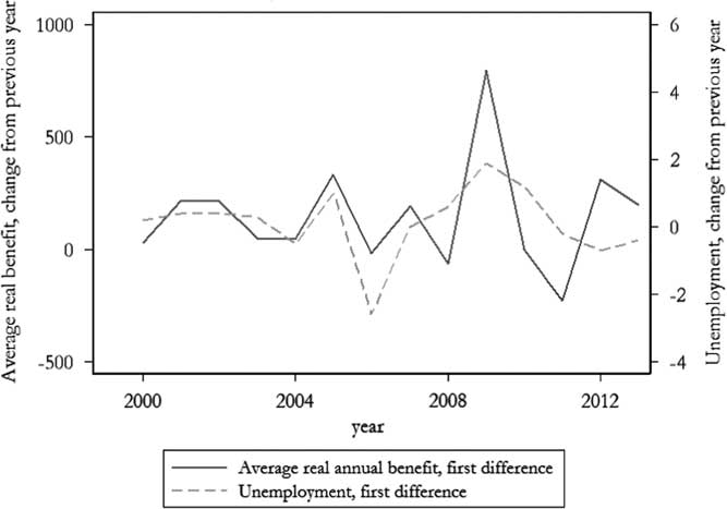
Which states have high benefit levels? The estimates suggest that five of the variables included in the model are important, but the impact of unemployment is particularly large. States with historically high growth in real per capita income are associated with higher average benefit levels, as expected. States with rising unemployment levels experience substantial growth in average benefits. The effect of unemployment swamps the other factors in the model: a 1 SD change in the first difference of unemployment (~1%) is associated with a more than $100 increase in annual average benefit levels (about a 0.75% increase in the average benefit). This finding reveals that the earnings history of new filers supports a higher benefit than the earnings history of earlier cohorts, even with any penalty related to claiming before full retirement age. The data are simply unambiguous about this result. Figure 6 plots the average difference in average benefits each year and the average difference in unemployment rates each year. The average benefit level surges upwards in periods of high unemployment and moves up at a slower rate when unemployment is low.
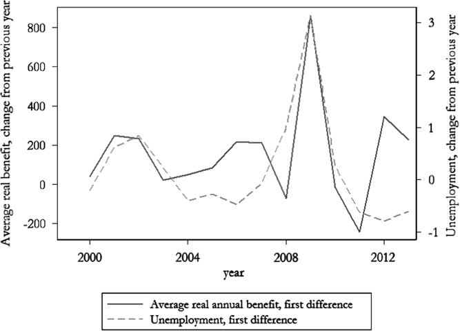
Figure 6 Unemployment and average real old-age benefit levels, first difference, 2000–2013
Using data for individual states can reveal how this process unfolds in different ways in different states. Figures 7 and 8 summarise the path of first difference in unemployment level and average benefits in Louisiana and Michigan. Note the different paths of each indicator in 2006. In Louisiana, unemployment falls and average real benefit falls by $18 (more accurately, changes in nominal benefits fail to keep pace with inflation). In Michigan, unemployment increases by a small amount and the average real benefit increases by over $200.

Figure 7 Unemployment and average real old-age benefit levels, first difference, 2000–2013. Note: State of Louisiana.
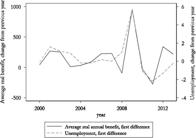
Figure 8 Unemployment and average real old-age benefit levels, first difference, 2000–2013. Note: State of Michigan.
To test the robustness of this result outside of the sample period, we collected data on average national unemployment and average national benefit increases from 1983 to 2014. The observed relationship between the first difference in real benefits levels and the first difference in unemployment was very close to the results in Table 1: an increase of just over $100 in average annual benefits for each 1% increase in unemployment. Finally, we also tested to see whether it was simply the huge spike in unemployment in 2009 that accounted for the impact of unemployment. We found that the impact of unemployment is positive and statistically significant if the sample is restricted to the period ending in 2007.
Other variables in the model also matter, but the impact is much lower. States with growing minority populations have benefits that grow faster than other states – a 1 SD increase in the first difference of the state proportion minority implies a $30 increase in average annual benefits. States with an increase in college completion will also see lower average benefits, inconsistent with our expectations. This is perhaps the most puzzling result we uncover – in places and at times that overall educational attainment falls, OA average benefits rise. Part of this is due to one year – 2011 – where Social Security average benefits decline in nearly all states, whereas the college completion measure increases by a large amount in almost all states. Overall, states with poorly educated and minority residents experiencing growing levels of unemployment will see average benefits climb; the new and large cohort of workers who elect to begin receiving Social Security OA payments qualifies for sometimes much higher benefits than current recipients. The growth rate of the senior population has no link to the level of average benefits.
Overall, the combination of insights from the two models reveals what explains state variation. In most cases, if a variable is positively associated with average benefits, it is negatively associated with coverage and vice versa. This is the case with real per capita income, minority population, poverty, senior population and college completion. When a high proportion of the state is covered, the average benefit is lower. When a smaller proportion of the state is covered, the average benefit is higher. The exceptions to this are unemployment and public sector worker participation. States where public sector employees are covered have both broader coverage and higher average benefits. Unemployment is positively associated with both coverage and benefit levels: states with rising unemployment have broader coverage and higher benefit levels and the effect of unemployment in both models is large.
Conclusion
When scholars discuss the welfare state and its capacity to mitigate economic insecurity, the United States is often viewed as an exception. Other advanced industrial societies, particularly in Western Europe, instituted social insurance programmes earlier and with universal benefits. Reviewing work in this tradition, one set of researchers concludes that “the image of American social policy is one of stinginess and backwardness” (Amenta, Bonastia and Caren Reference Amenta, Bonastia and Caren2001, 215). In this context, the OA programme is an anomaly, one component of what Quadagno (Reference Quadagno1987) labels the “bifurcated” welfare state – where a majority of worthy (elderly) beneficiaries are differentiated from a minority of unworthy (single, poor, mother) beneficiaries. As the OA programme is popular, the level of financial support – measured by the proportion of the economy or the proportion of the federal budget devoted to pensions for the elderly – places the United States at the average among Organization for Economic Co-Operation and Development (OECD) nations: about 17% of the total federal budget and 7% of the total economy (OECD 2013).
However, despite a structure designed to ensure equitable treatment independent of place of residence, the programme impacts the US states in surprisingly different ways. The empirical finding that is most robust – across model specifications, measures of OA expenditures and choice of estimator – is the link between unemployment and OA expenditures. In states with growing unemployment, the proportion of covered seniors expands, average benefits expand and, as a consequence, the level of OA expenditures directed to the state expands. This result suggests that OA expenditures do not simply lift seniors out of poverty. The OA programme is a critical component of response to recession and labour market disruption. The estimates presented here do not permit us to specify the effect of these expenditures on overall performance of the state economy or show exactly how these expenditures mitigate the effects of a recession, but the results do suggest an important and unexpected impact of OA programme expenditures. Future research could exploit individual-level or household-level data – SSA administrative data or the Survey of Income and Program Participation – to determine how spells of unemployment increase the probability of triggering OA benefits and which workers (low or high income, above or below full retirement age, for instance) are most likely to initiate OA benefits during a recession.
Economists expect that federal expenditures will increase as the economy deteriorates. Unemployment insurance payments and nutrition assistance programmes are typically identified as the automatic stabilisers that require no or few statutory triggers to respond to an economic crisis (Zilak et al. Reference Zilak, Gundersen and Figlio2003; Congressional Budget Office 2013). However, as a haven for older workers displaced by long-term job losses, the Social Security OA programme serves much the same function. The programme expands in scope and in average benefits during recessions, in states where unemployment is growing at a particularly fast rate. This is a poorly understood but important feature of the Social Security programmes. The results presented above suggest that there are opportunities to investigate the multiple ways that the stream of benefits from the OA programme impacts state economic performance. For instance, if coverage expands to large numbers of newly unemployed workers, then the impact of unemployment on economic consumption could be blunted. In addition, if unemployed workers trigger OA benefits, then state unemployment insurance funds might see some short-term relief during a harsh recession. Future research could quantify the size and duration of these aggregate effects.
Research on state-to-state variation in federal expenditures has largely and understandably focused on federal programmes that permit some discretionary actions by state officials. The governor, the legislature or administrative actors can implement federal programmes at the state level in ways that influence the flow of resources to the state. The OA programme is a reminder that, even in the absence of this type of discretion, the flow of resources can be quite uneven and behave in entirely unexpected ways. In states with a booming economy – lower unemployment – workers defer entry to Social Security. In states with a deteriorating economy – higher unemployment – workers use Social Security as an important safety net. The wave of new filings for benefits early in the Great Recession took the SSA by surprise, but the underlying dynamic that produced this spike is not new or idiosyncratic. The Social Security OA programme serves not only the original intended goal of taking retired seniors out of poverty, but perhaps an unintentional goal of shifting federal expenditures to the places where unemployment is most severe.
Acknowledgement
The authors would like to thank Gunther Hega, Susan Hoffmann, Wei-Chiao Huang and the anonymous reviewers for comments and feedback. A preliminary version of this work was presented at the annual meetings of the Midwest Political Science Association in 2012.
Supplementary material
To view supplementary material for this article, please visit https://doi.org/10.1017/S0143814X17000277
Appendix I. Data sources and descriptive statistics
Data sources
Pension plans. Proportion of state and local government workers covered by Social Security
Public Plans Data. Center for Retirement Research at Boston College, the Center for State and Local Government Excellence and the National Association of State Retirement Administrators. http://publicplansdata.org/
Social Security Old-Age (OA) programme beneficiaries by state
Table 5.J.2 Social Security Bulletin. Annual Statistical Supplement. Various Years
Social Security Old-Age (OA) programme expenditures by state
Table 5.J.1 Social Security Bulletin. Annual Statistical Supplement. Various Years
State college completion rate
Bureau of the Census. 1990, Census of Population; 2000, Census of Population; 2006–13, American Community Survey, Single Year Estimates and ACS Fact Finder.
2001–2005 estimated by authors from 2000 and 2006–2010 observations.
State manufacturing employment
Bureau of Labor Statistics. State and Metro Area Employment, Hours, & Earnings (download.bls.gov/pub/time.series/sa/)
State minority population
Bureau of the Census. 2010–2014 (July 1 estimates) American Fact Finder; 2000-2009, Intercensal Estimates of the Resident Population by Sex, Race, and Hispanic Origin for States: April 1, 2000 to July 1, 2010
State per capita income
Bureau of Economic Analysis, Regional Economic Accounts (www.bea.gov/iTable/)
State population, 65 and over
Bureau of the Census. 2011–2014. American Community Survey; 2000–2010. Intercensal Estimates of the Resident Population by Sex and Age for States: April 1, 2000 to July 1, 2010; 1999. Estimated by authors from 2000 and 2001 data.
State population, total
Bureau of the Census. 2011–2014. American Fact Finder. July 1 estimates; 1999–2009. Intercensal Estimates of the Resident Population for the United States, Regions, States, and Puerto Rico: April 1, 2000 to July 1, 2010
State poverty rates
Bureau of the Census, Small Area Income and Poverty Estimates (census.gov/did/www/saipe)
State unemployment rates
Bureau of Labor Statistics, Local Area Unemployment Statistics (download.bls.gov/pub/time.series/la/)
Descriptive statistics
Average annual state OA expenditures per beneficiary (benefit level)
Mean and range: $12,528 ($10,421–$15,365)
Average first difference: $158
Percentage of state over-65 population receiving benefits (coverage):
Mean and range: 89.7 (78.5–98.7)
Average first difference: 0.14
Percent change in over-65 population, annual, by state
Mean and range: 1.9 (−3.6–6.2)
Average first difference: 0.22
Percentage of state population that is non-white:
Mean and range: 17.9 (2.7–74.3)
Average first difference: 0.04
State college completion rates, percentage, 25 years and older
Mean and range: 26.5 (14.6 –3.3)
Average first difference: 0.50
State poverty rates, percentage
Mean and range: 12.7 (5.6–23.1)
Average first difference: 0.24
State real per capita income, in thousands of 2014 dollars
Mean and range: 41.554 (28.800–63.731)
Average first difference: 0.377 ($377)
State unemployment rate, annual average, percent:
Mean and range: 5.8 (2.3–13.7)
Average first difference: 0.18
State and local government workers covered by Social Security, proportion
Mean and range: 0.807 (0.0–1.0)
Average first difference: n/a