Motivating a dynamic approach to modelling public policy

A growing body of public policy theories argues that politics is a terrain that is restructured over time. A prime example is the work of Baumgartner, Jones and colleagues, which claims that over time most policy areas may be subject to changes in policymakers’ focus (Jones Reference Jones1994; Baumgartner and Jones Reference Baumgartner and Jones2002; Jones and Baumgartner Reference Jones and Baumgartner2005; Baumgartner and Jones Reference Baumgartner and Jones2015). As a consequence, no single logic of policymaking and no single frame of reference lasts forever. Historical contingencies are fundamental to politics, and the threshold for action even within a single policy area may change over time, as the weighting of policy problems is dynamic (Jones and Baumgartner Reference Jones and Baumgartner2005, 90–91).

Other major contributions to the study of public policy have a different conceptualisation, description and explanation of policy change, but they share the important implication that the determinants of public policy may change over time. One example is the Advocacy Coalition Framework, according to which every coalition of policymakers contains secondary aspects, policy core beliefs and so-called deep core beliefs. Secondary aspects comprise a large set of narrower beliefs of the policymakers concerning, for instance, their evaluation of relevant problems and performances within a policy subsystem as well as their preferences regarding regulations or budgetary allocations (Sabatier Reference Sabatier1998). Policy core beliefs refer to a coalition’s basic normative commitments and causal perceptions across an entire policy domain, and deep core beliefs include basic ontological and normative beliefs operating across almost all policy domains (see also Weible et al. Reference Weible, Sabatier and McQueen2009, Reference Weible, Sabatier, Jenkins-Smith, Nohrstedt, Henry and deLeon2011). When it comes to the core beliefs, these are assumed to be very stable, though not time-invariant. Even if changes mainly involve secondary aspects, this may, for instance, have implications for the relative importance of various causal factors within a given policy domain (Sabatier Reference Sabatier1998, 104).

Another example is Hall’s (Reference Hall1993) seminal work on social learning and policy paradigms, according to which both the instruments and goals of public policymaking may change over time (see also Campbell Reference Campbell2002; Blyth Reference Blyth2013; Princen and ’t Hart Reference Princen and ’t Hart2014). In Hall’s thinking, policy change comes in three basic types. First-order changes are policy shifts that leave the larger policy regime in place, for instance, changing the minimum lending rate or fiscal stance to adjust macroeconomic policy. In Hall’s analogy, first-order changes adjust the settings on the “instruments” of policymaking. Second-order changes, on the other hand, replace the instruments themselves (Hall Reference Hall1993, 278–279) – in the example of macroeconomic policy, changes in the system of monetary control or adopting or abandoning strict targets for monetary growth would be second-order changes. Third-order changes alter the instruments, their settings and the hierarchy of goals behind policy. Hall’s prime example of a third-order change is the paradigmatic shift in British macroeconomic policy in the 1970s and 1980s from Keynesian to monetarist modes of economic regulation.

Just as changes in deep core beliefs are assumed to be rare according to the ACF, paradigmatic third-order changes are very rare according to Hall’s theory. It is important to note, however, that even second-order changes or, in the parlance of ACF, changes in policy core beliefs will most likely be reflected in time-varying relationships in time series models of public policy. A second-order change, for instance, reflects an alternation of the hierarchy of goals behind policy (Hall Reference Hall1993, 282), and a change in the policy core beliefs of policymakers may involve a change of their causal perceptions of a policy domain (Sabatier Reference Sabatier1998, 103). Put differently, if the decisionmakers’ causal understanding of the relationship between problems and solutions changes within policy domains such as defense, welfare, transportation or environmental policies, then the relationship between x and y probably changes as well.Footnote ¹

Across the different theoretical approaches and different subfields of policy research there is a consensus that the dynamic implications of these theories are not adequately analysed by using standard time series regression techniques (Jones and Baumgartner Reference Jones and Baumgartner2005; Hall Reference Hall2006, 90–91). The basic problem with standard regression models is simple. If relationships between x and y are time-variant then the basic regression assumption of unit homogeneity is violated. In other words, changes in the value of an explanatory variable, x, will not produce corresponding changes in the value of the policy output variable, y, of the same magnitude, or even direction, across all time (cf. Hall Reference Hall2003, 382).

As we will discuss in detail below, common responses to this problem are to divide time series into epochs or to specify interaction terms conditioning the relationship between x and y. The problem, however, is that such approaches require strong theories about when the relationship between x and y transforms. Often, as argued by Jones and Baumgartner (Reference Jones and Baumgartner2005, 23), we have no a priori idea when such changes take place: “If we look at a series of policy activities, as we do for crime, social welfare, and other policy areas, we find clear evidence of self-reinforcing changes. While it is possible to model such complex series, how does one know in advance when these interactions will occur?”. Similarly, in a recent review of the Advocacy Coalition Framework, Jenkins-Smith et al. (Reference Jenkins-Smith, Nohrstedt, Weible and Sabatier2014) identify four major pathways to policy change, each of which may be a necessary but not sufficient source of change in policy core beliefs. Finally, even if theory does contain a strong prediction of the timing of a transformative policy change, we need a flexible estimation model in order to be able to falsify or support that prediction empirically.

This discontent with standard time series approaches has led policy scholars to advocate alternative methods that are better aligned with their theoretical approaches to public policy. One example is systematic process tracing (Hall Reference Hall2003), which can be a strong approach to identifying causal processes leading to a political outcome. Another example is the stochastic process approach advocated by Jones and Baumgartner (Reference Jones and Baumgartner2005). A major advantage of a stochastic process approach is the focus on entire distributions of data (not only mean and variance) and the lack of assumptions required. Yet, we also set aside important information by using these approaches: giving up the ability to examine directly the relationships between changes in (potentially multiple) policy determinants and changes in policy outputs or ignoring the chronology of our data. Thus, we sympathise with the expansion of methods better aligned with the ontology of the major public policy theories, but we believe there also is a strong case for improving the statistical time-series analysis of policy dynamics. In the next section, we motivate the adoption of a flexible approach to time series policy analysis suited to uncovering time-varying relationships.

Estimating dynamic relationships in public policy research

Given the goal of examining dynamic relationships between an explanatory variable (x) and a policy output (y), we propose that the hypothetical ideal statistical model has two features. First, it would estimate variation in x’s relationship to y over time (t), directly from the data. Formally, we might write,

(1) $$y_{t} \,{\equals}\,x_{t} \beta _{t} {\plus}{\epsilon}_{t} $$

The t subscript on β _t indicates a new parameter value is estimated each time period, indicating how the relationship between x _t and y _t changes or remains constant. Such a model’s estimates would be guided by the data, as they would be estimated directly.

Second, an ideal model would estimate β _t in a way that respects its chronology. That is, given the emphasis theory places on history and path dependence in public policy (cf. Jones and Baumgartner Reference Jones and Baumgartner2005, 49), we must not assume β _t′ is completely independent of β _t″ (e.g. β _t is not independent of β _t−1 or of β _t−4, etc.).

The main barrier to this idealised model is identification – that is, its parameters outnumber its data points and therefore, even with infinitely long time series, one cannot estimate them without making additional assumptions. The time series regression modelling toolkit contains many second-best alternatives, however. We argue that time-varying relationships of the form presented in Equation 1 are common in policy studies, but that the tools commonly used to study them provide answers that are not guided only by the data nor do they account for the data’s chronology.

In this section, we provide an accessible introduction to a well-studied method for estimating dynamic relationships that meets both criteria; we review the advantages these criteria hold for public policy research; and we consider the method’s strengths relative to commonly used approaches. Namely, we propose that researchers examining policy changes featuring time-varying relationships of this sort consider a class of modelling techniques known as DLM (Kim and Nelson Reference Kim and Nelson2000; Mcavoy Reference Mcavoy2006; Shumway and Stoffer Reference Shumway and Stoffer2010) or flexible least squares (Kalaba and Tesfatsion Reference Kalaba and Tesfatsion1988; Wood Reference Wood2000).Footnote ² The difference between the two, for our purposes, lies in assumptions about the distribution of errors in DLMs. We refer to DLMs throughout as we adopt this formulation to estimate uncertainty.

In what follows, we make the case for more widely adopting DLMs for studying policy change. It is worth reiterating that DLMs, a subset of the broader category of state-space models, are not unknown in political science (Gerber and Green Reference Gerber and Green1998; Green et al. Reference Green, Gerber and de Boef1999; Mitchell et al. Reference Mitchell, Gates and Hegre1999; Brandt et al. Reference Brandt, Williams, Fordham and Pollins2000; Wood Reference Wood2000; Mcavoy Reference Mcavoy2006; Enns and McAvoy Reference Enns and McAvoy2011; Fariss Reference Fariss2014). Indeed, Beck (Reference Beck1983) argued that the approach had strong advantages for theory testing and should be added to the arsenal of those who work with time series data. Though they have been applied to study public opinion and international conflict, specifically to deal with the kind of effect heterogeneity that we are concerned with, the method has not gained traction in studies of public policy. Potential applications are, nevertheless, widespread. The goal of estimating time-varying relationships originally motivated state-space models’ development in physics and, more recently, has encouraged their adoption and popularisation especially in economics and finance (for background, see: Kim and Nelson Reference Kim and Nelson2000; Mergner Reference Mergner2009).

Returning to Equation 1’s hypothetical model, the DLM recovers estimates of time-varying effect coefficients, that is, β _t , provided some scaffolding in the way of assumptions about how β _t changes with time. Specifically, in a DLM β _t is a realisation of an underlying “state” that varies as a Markov chain over time. This formulation ensures identification and reflects one of the principles we proposed above: that dynamic relationships should be estimated in a way that respects the data’s chronology. As we will see, DLMs can flexibly return time-constant coefficient estimates where appropriate or detect the presence of dynamics. A simple DLM built to emulate Equation 1 might be structured as follows:

(2) $$y_{t} \,{\equals}\,{\mib X}_{{\mib t}} \bibeta_{{\mib t}} {\plus}v_{\bib t} $$

$$v_{t} \!\sim\!i.i.d.(0,\sigma _{v}^{2} )$$

(3) $$\bibeta_{{\mib t}} \,{\equals}\, \bibeta_{{{\mib t}{\minus}{\bf 1}}} {\plus}{\mib w}_{{\mib t}} $$

$${\mib w}_{{\mib t}} \,\sim\,i.i.d.(0,Q)$$

The first line, Equation 2, is called the measurement equation. Inputs to the policy-making process in vector X _t influence policy y _t via the vector of time-varying effect coefficients β _t . The disturbances, v _t , are independent zero-mean Gaussian noise with variance $$\sigma _{v}^{2} $$ . The third line, Equation 3, is the state equation. Here, the effect coefficients, β _t , are modelled as an unobserved state varying in a random walk over time. The state disturbances, in vector w _t , are also mean-zero Gaussian noise with covariance matrix Q and are uncorrelated to v _t .

Equations 2 and 3 demonstrate how a DLM respects the goal of producing estimates guided by the data and accounting for chronology. Estimates of β _t come directly from the data and are linked over time in Equation 3. This structure allows estimates of β _t to be informed by the whole time series, while still ensuring them flexibility to reflect any pattern of variation indicated by the data. What value added does this bring to policy studies examining time-varying relationships? We suggest several. For one, estimates that depend only on the data limit the assumptions analysts must make. As we review below, many methods for identifying dynamic relationships must justify not only their measurements, cases and modelling choices – as in any empirical analysis – but also must justify a priori expectations about the timing of shifts in relationships or the use of statistical tests to pinpoint them.

Perhaps more importantly, estimates of dynamic relationships arising from the data enrich our ability to falsify hypotheses. Hypotheses about time-varying relationships may be falsified if a relationship does or does not exist, does or does not vary, or does or does not vary at a particular time. DLMs can speak to these criteria simultaneously. This has the advantage of avoiding bias from or corrections for multiple testing if the analyst wishes to consider different null hypotheses. Furthermore, since DLMs feature time-connected estimates of β _t , they utilise all the information in the data, maximising the statistical power of the estimates and using information from the full time series to estimate each coefficient.

Consider, briefly, advantages DLMs enjoy relative to other approaches to estimating time-varying relationships. A common approach to this problem is to estimate variation in effect parameters by subdividing time series into shorter epochs and running separate regressions on each subset of the data or, similarly, including interaction terms for epochs. This encounters several weaknesses. The first relates to statistical power. Subdividing time series necessarily weakens inferences by working with smaller data subsamples, increasing risks of both Type I and Type II errors. Second, and potentially more challenging, subdividing requires analysts to identify and motivate the choice of relevant time periods a priori. A principled choice of time periods may be available for certain tests, but considering more than one choice ventures into multiple testing. Furthermore, subdividing still forces analysts to assume effect parameters are constant within epochs.

Low statistical power is also a difficulty for CUSUM and CUSUMSQ plots as tests for parameter stability (Wood Reference Wood2000; Baltagi Reference Baltagi2011). These plot functions of cumulative sums of residuals to identify shifts in parameters. Although this approach is estimated directly from the data, it falls short of the criterion of time-connectedness. Having identified a change in a parameter via CUSUM plotting, this method provides no guidance in estimating or accounting for temporal dependency in parameter shifts.

Difficulties in motivating a priori information also apply to the Chow test, which can reveal if an effect parameter shift occurs at a particular point (Beck Reference Beck1983; Wood Reference Wood2000) – a point the analyst identifies. Again, having identified potential change points, there is no clear method for estimating parameter changes that respect time-dependence.

Concerns with statistical inefficiency and motivating a priori information also extend to moving window analysis (Kwon and Pontusson Reference Kwon and Pontusson2010; Finseraas and Vernby Reference Finseraas and Vernby2011). Moving window analyses ignore large portions of data to estimate each bit of dynamics in effect coefficients. Although eventually all data are considered, observations at the beginning and end of time series are less influential than those in the middle, and each individual estimation has less statistical power than would be achieved using all data. Furthermore, decisions such as window size and which observations to include in each analysis can be consequential for the results, and yet are left to the analyst’s choice.

Still more systematic methods include multivariate generalised autoregressive conditional heteroskedasticity models (MV-GARCH) or dynamic conditional correlations (DCC) (Engle Reference Engle2002; Lebo and Box-Steffensmeier Reference Lebo and Box-Steffensmeier2008). These dynamically estimate the covariance matrix of multivariate time series using a framework adapted from GARCH modelling. This is a powerful method for identifying a certain type of dynamics, namely in correlations. Although they satisfy our proposed criteria of being data-driven and (partially) time-connected, they require quite large data sets and address themselves to correlations and not to the explanatory modelling problem described in Equation 1.Footnote ³

There are, of course, limitations to DLMs. As in any parametric modelling, the assumptions underlying the method matter and model reliability is better confirmed than assumed. Therefore, we provide guidance in probing the conditions for applying DLMs by using appropriate diagnostics and demonstrate how to use in-sample predictions and simulations to check the appropriateness of DLMs for a given application.Footnote ⁴

Estimating a DLM

A standard approach to estimating DLMs like the one we describe above is via a combination of maximum likelihood and the Kalman filter (Kim and Nelson Reference Kim and Nelson2000; Commandeur and Koopman Reference Commandeur and Koopman2007; Petris et al. Reference Petris, Petrone and Campagnoli2009; Shumway and Stoffer Reference Shumway and Stoffer2010), though Bayesian estimation methods are also common (Petris et al. Reference Petris, Petrone and Campagnoli2009; Shumway and Stoffer Reference Shumway and Stoffer2010). We describe here how to apply the former approach to estimate a DLM. To illustrate the method, we walk through the process of estimating the model described in Equations 2 and 3 – an example of a dynamic model of the impact of various influences on some policy output in a single time series.

DLMs are estimated recursively. Referring to Equation 3, at each time t, β _{t −1} serves as our expectation of the new period’s value of β _t , conditional on the information observed up to time t−1. On the basis of this conditional expectation for β _t , we calculate a prediction for the outcome in time t: $$\hat{y}_{t} $$ . The error in this prediction, $$y_{t} {\minus}\hat{y}_{t} $$ , is used to update our final estimate of β _t , such that larger errors provoke larger shifts in coefficient estimates. The recursion proceeds sequentially from time 1 through time n. This means that at any point, t, all past information about the underlying state is summarised in the point estimates, β _t , and their covariance matrix at time t−1.

Shifts in the coefficient estimates each period are moderated by the ratio of uncertainty regarding the estimates of β _t to the total overall estimation uncertainty in the model (including that from β _t ). Where uncertainty about β _t is a larger share of overall model uncertainty, this ratio – termed Kalman gain – is closer to one. Updates to the coefficients become more responsive to that period’s prediction error as the Kalman gain approaches one. A formal definition of the Kalman gain and detailed estimating equations are provided in the Online Appendix A.

The final step in the estimation is to smooth the time-varying state estimates using information from the full time series. Kalman smoothing utilises the same approach as the filter, but is run in reverse. Recall that when filtering at each time period, t, all information about the unobserved states up to period t is summarised in the point estimates and associated uncertainty of last period’s state estimates: β _t−1 . The smoother, by running in reverse from time T back to time 1, updates each period’s estimate of β _t conditional on all information in the model. Filtering alone is used for applications in which the goal is to forecast future outcomes, whereas smoothing is applied in applications aimed at making inferences about effect parameters. In public policy, our inferences are generally of the latter type, addressing effect estimates in fixed time series. For that goal, filtering by itself suffers several weaknesses relative to filtering plus smoothing. First, changes in filtered parameter estimates lag changes in smoothed parameter estimates (Commandeur and Koopman Reference Commandeur and Koopman2007, 85–89). This is a product of the estimation process and does not negatively impact filtering’s predictive accuracy. However, the lagged filtered parameter estimates are out of sync with the best estimate of the actual pattern in the data – a situation smoothing resolves. Second, filtering overstates uncertainty in early estimates of β _t , as chronologically earlier observations are estimated using fewer data points. Third, filtering can over- or understate the magnitude of shifts in coefficient estimates relative to smoothed estimates. In sum, smoothing provides the more accurate inference for β _t because it uses more information than filtering alone (Kim and Nelson Reference Kim and Nelson2000, 27). Furthermore, as we have argued our estimates of β _t must not be fully independent of one another, we prefer combined filtering and smoothing.Footnote ⁵

Final effect coefficient estimates are these smoothed time-varying coefficients. The recursive estimation procedure is identified conditional on a set of starting values for β ( β ₀) and estimates of Q, $$\sigma _{v}^{2} $$ and the starting value of the covariance matrix of innovations, ∑₀. These are estimated via maximum likelihood. The process begins with initial values for each of these latter parameters, and then each β _t is estimated from time 1 using the Kalman filter followed by smoothing.

As can be seen in Equation 2, the DLM also relies on assumptions about the independence, normality and homoskedasticity of errors. Violations of these assumptions can be checked straightforwardly by examining standardised residuals from an estimated model (see, for example, Commandeur and Koopman Reference Commandeur and Koopman2007, 90–96). An assumption common to standard time series techniques that is not encoded in the DLM framework, is stationarity. That is, our methods often require we assume that statistical features of time series inputs to the model, like their mean and variance, do not vary over time. Such variation cannot be captured by static coefficient estimates. However, since coefficients vary with time in the DLM data used in such applications need not exhibit stationarity (Commandeur and Koopman Reference Commandeur and Koopman2007, 134; see also, Petris et al. Reference Petris, Petrone and Campagnoli2009, 34, 115).

The basic DLM described here can also be extended to accommodate a variety of alternative settings, for example, autoregressive processes, moving averages, constraining certain parameters to be constant, generalised linear models for nonnormally distributed response variables and others (Petris et al. Reference Petris, Petrone and Campagnoli2009; Shumway and Stoffer Reference Shumway and Stoffer2010). As we show later, the DLM can also be extended to panel data.

Statistical software for estimating DLMs is widely available. An excellent starting point for applying them in the reader’s own work is to review volume 41 of the Journal of Statistical Software, a special issue on state-space estimation in STATA, R, SAS, RATS and other statistical software packages. The results we present are estimated using the “dlm” library for R (Petris Reference Petris2010), which is one of several options in R (Petris and Petrone Reference Petris and Petrone2011; Tusell Reference Tusell2011).

We turn now to applying DLMs to a real empirical case in policy studies to demonstrate its usefulness and potential applications.

A DLM analysis of US defense policy

We illustrate the dynamic modelling approach using real data on US defense spending, applying the technique to test for dynamic relationships between the explanatory variables and policy outputs. US defense spending offers an attractive test ground for several reasons. First, although the use of public spending as a policy indicator has been subject to some debate, the defense area is one where changes in spending have often been taken as evidence of important changes in defense policies (see e.g. Hartley and Russett Reference Hartley and Russett1992; Wlezien Reference Wlezien1996; True Reference True2002). Second, many studies have tried to model time series of US defense spending, which provides some direction for our choice of explanatory variables. The many defense studies partly reflect a genuine interest in this policy field during the Cold War, and partly reflect the availability of rather reliable and long time series within this policy field. A broad range of drivers of US defense spending have been examined in these time series studies including election cycles (Nincic and Cusack Reference Nincic and Cusack1979; Cusack and Ward Reference Cusack and Ward1981; Zuk and Woodbury Reference Zuk and Woodbury1986; Kamlet and Mowery Reference Kamlet and Mowery1987), measures of unemployment (Griffin et al. Reference Griffin, Wallace and Devine1982; Kiewiet and McCubbins Reference Kiewiet and McCubbins1991; Cusack Reference Cusack1992; Majeski Reference Majeski1992; Su et al. Reference Su, Kamlet and Mowery1993), arms races (Ostrom Reference Ostrom1977; Ostrom Reference Ostrom1978; Ostrom and Marra Reference Ostrom and Marra1986; Correa and Kim Reference Correa and Kim1992), inertia (Ostrom Reference Ostrom1977; Majeski Reference Majeski1983; Correa and Kim Reference Correa and Kim1992) and public opinion (Hartley and Russett Reference Hartley and Russett1992; Higgs and Kilduff Reference Higgs and Kilduff1993; Wlezien Reference Wlezien1996). A more complete overview of variables and measures adopted in previous work is included in Table A.1 in the Online Appendix B.Footnote ⁶

The US defense spending studies disagree with respect to several model assumptions, including the choice of explanatory variables and the exact specification of the dependent variable. Nevertheless, common to virtually all of them is the modelling assumption that relationships are invariant over time. The assumption is so uncontested that it is not given serious consideration in most previous defense spending studies. This is a further argument for investigating whether the approach advocated in this article is able to detect dynamic relationships within such a well-researched field as US defense spending. Only one study we know of escapes this characterisation of the field. True (Reference True2002) examined US defense spending over several decades and found that the relationship between defense spending and prior spending, international tensions and wars, and US intelligence estimates of Soviet defense spending showed some evidence of changing over time.

To reach this conclusion, True (Reference True2002) split the time series into two periods, 1966–1979 and 1980–1992. Given the limitations with this research strategy we reviewed above, we reevaluate True’s findings using a DLM to detect dynamics in effect coefficients over time. We take our analysis of US defense spending in two stages. First, using the dynamic estimation approach advocated here, we analyse US spending based on similar data as True (Reference True2002), but for a longer time period, 1956–2010.Footnote ⁷ Second, we broaden the range of explanatory variables in light of the outcomes of the model 1 analysis and in light of the broader literature on US defense spending. We hold constant across both model specifications the response variable: the percentage of annual change in US defense budget authority.Footnote ⁸ Thus, we collected similar data but for an expanded period, 1956–2010.

Table 1 provides an overview of the range and specification of explanatory variables used in models 1 and 2, respectively. As argued above, the dominant theories of public policy do not generally offer guidance about when relationships change, only that they may change over time. For instance, partisan alignments around the defense issue may change over time, reflecting new problem developments, a new understanding of the issue and/or new linkages of defense to other issues such as terrorism, the economy and employment. Similarly, the importance of public opinion on this issue relative to other drivers of policymaking may change over time resulting in a dynamic impact of public opinion on defense spending. On the other hand, it could also be the case that such transformative change is less prevalent than claimed by theories of public policy. The previous time series analyses on defense spending do not tell us much about this question and it is therefore warranted to initiate a closer inspection of this question utilising the rich time series data on US defense spending.

Table 1 Explanatory variables from previous research

Note: A more comprehensive list of explanatory variables from previous research can be found in the Online Appendix B. US=United States; GDP=gross domestic product.

^* This model builds on True (Reference True2002).

^† This model builds on the outcome of the model 1 analysis as well as the broader literature on defense spending (see also Table A.1 in the Online Appendix B).

^‡ Heffington, Colton, Brandon Beomseob Park, and Laron K Williams. (2017) The “Most Important Problem” Dataset (MIPD): a new dataset on American issue importance. Conflict Management and Peace Science. [dataset]

Summary statistics for all variables in both models can be found in the Online Appendix C. For both models, we summarise results by plotting estimated effect coefficients over time with confidence intervals. Since the model estimates coefficients and standard errors for each year (observation) in the data, coefficient tables are impractical. Results are most easily interpreted graphically. Both models use data standardised by subtracting variable means and dividing by one standard deviation.Footnote ⁹ As a result, both models also exclude constants. For assessments of both models’ in-sample predictive accuracy, see the Online Appendix E.

Results: model 1

Dynamic coefficient estimates from our first model specification are plotted in Figure 1. There is some initial evidence here that influences on public spending do not have constant effects over time. Periods of war and international tension are not consistently related to changes in defense spending, for example, with certain periods associated with more and certain periods with less spending. Furthermore, lagged real defense spending (in levels) is not consistently negatively associated with subsequent spending changes, which indicates a dynamic adjustment process (see De Boef and Keele Reference De Boef and Keele2008). Whereas a negative coefficient may be interpreted as reflecting negative feedback, with the defense budget regressing back to its “normal” level, a positive coefficient would signal positive feedback in the sense that high budgets would be followed by further increases (see also Wood and Doan Reference Wood and Doan2003). Figure 1 does not show a full shift from negative to positive feedback, but the varying effects over time of the lagged spending measure may be interpreted as evidence in support of the emphasis on changing feedback processes in the punctuated equilibrium theory (Baumgartner and Jones Reference Baumgartner and Jones2002).

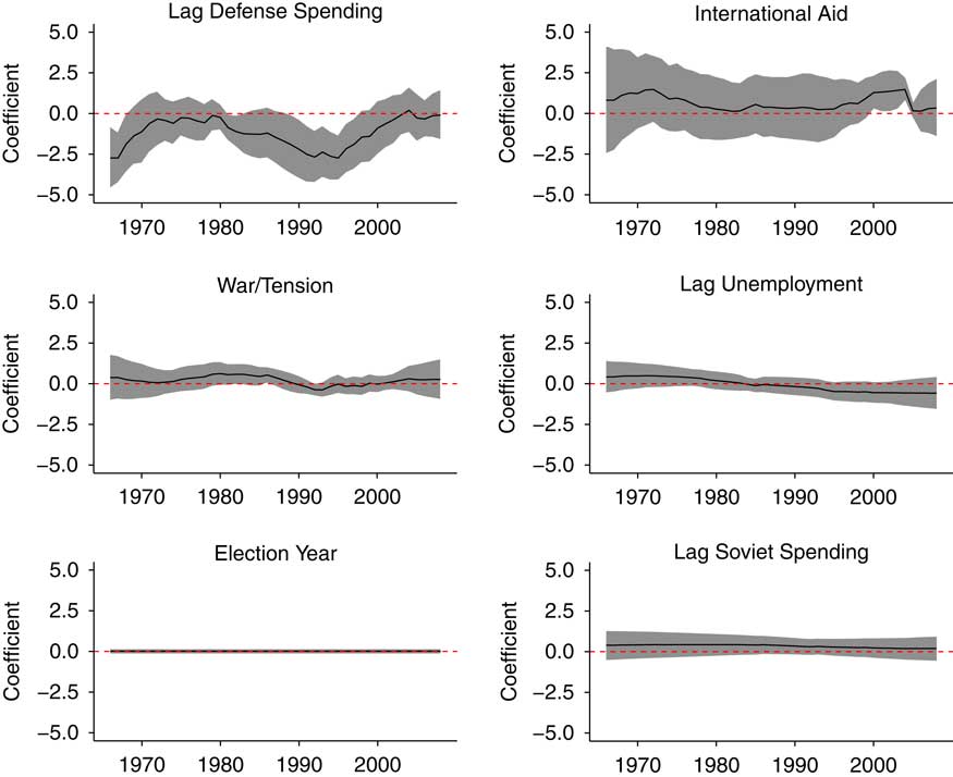
Figure 1 Estimated time-varying coefficients from model 1. Note: Effect coefficients are plotted over time. The solid line indicates the point estimate for the coefficient each period, whereas grey areas are 95% confidence intervals. The dashed horizontal line indicates 0. Where the grey area overlaps the dashed line, estimates are not statistically significant by conventional standards.

The rest of the estimates from the model show little evidence of dynamic effects. International aid demonstrates a brief positive association with defense spending in the first decade of the 21st century. This largely reconfirms True’s (Reference True2002) null finding regarding his hypothesis that international aid and military spending were determined in coordination. The period of our data also present in his analysis shows virtually no evidence in favour of this. Lagged unemployment shows statistically indistinguishable effects throughout, despite its mean estimated effect crossing the zero line during our period of analysis. The effects of both lagged Soviet defense spending and the election year indicator are basically constant and statistically indistinguishable from zero.

As the combination of relatively short time series and numerous parameters being estimated places high demands on our limited amount of data, we may improve our estimates if we can eliminate unimportant information from the model. Thus, we now turn to our revised model specification.

Results: model 2

In our second model, plotted in Figure 2, we see more suggestive evidence of dynamic effects over time. The results in this second model specification are estimated with greater certainty than the first and further sharpen some of the trends glimpsed in the first model. First, consistent with results in Figure 1, Figure 2 shows lagged defense spending is only sometimes negatively associated with percentage change in defense spending. Substantially, the dynamic estimates on lagged defense spending suggest that during the second half of the 1980s and through most of the 1990s the defense budget was regressing back to a “normal” level following a peak at the height of the Cold War. That is, the higher than average lagged spending levels in this period had a negative relationship to spending changes, and, indeed, the defense budget decreased annually from 1986 through 1998.

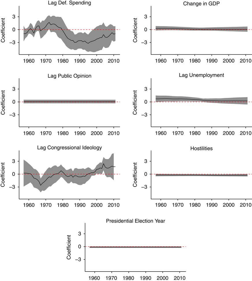
Figure 2 Estimated time-varying coefficients from model 2. Note: Effect coefficients are plotted over time. The solid line indicates the point estimate for the coefficient each period, whereas grey areas are 95% confidence intervals. The dashed horizontal line indicates 0. Where the grey area overlaps the dashed line, estimates are not statistically significant by conventional standards. GDP=gross domestic product.

Second, international hostilities display less dynamics than effects for True’s war and tensions indicator in the previous model, and yet it reaches negative statistical significance around the same time as the war/tension indicator – in the early 1990s. Although perhaps counter to intuition, the negative association between intensity of US participation in foreign hostilities and defense spending changes is likely meaningful here. Hostilities vary annually even during periods of international tension and are, therefore, measured more finely than a simple indicator. However, the summary statistics show it does not vary widely – US participation in militarised interstate disputes peaks several times during our period of analysis. Therefore, these estimates tell us that, despite an uptick in US participation in militarised interstate disputes in the 1990s, the period of hostilities following the end of the Cold War coincided with decreasing military spending, in contrast to the rest of the time series.

Third, the perhaps most noteworthy result in Figure 2 is that the effect of political preferences in the House of Representatives actually changes its direction over time. In contrast with classic conceptions of party positions on the defense issue, a more conservative House ideology had a negative association with changes in defense spending in the 1960s. The estimate became indistinguishable from zero until the late 1990s, and then the association reversed so that more conservative House ideology was related to greater spending through the first few years of the new century. These results indicate that partisan politics intrudes into defense spending changes only irregularly and in changing ways over time. Furthermore, the effects can be decisive. At its greatest positive point, in 2004, a 1 SD shift in House ideology towards conservatism would have an estimated effect of increasing defense spending by around 20%. The actual shift in House ideology that year was around one-fourth of a standard deviation towards the conservative side. At its most negative, in 1967, a shift towards conservatism in the House was associated with an even greater in magnitude drop in defense spending.

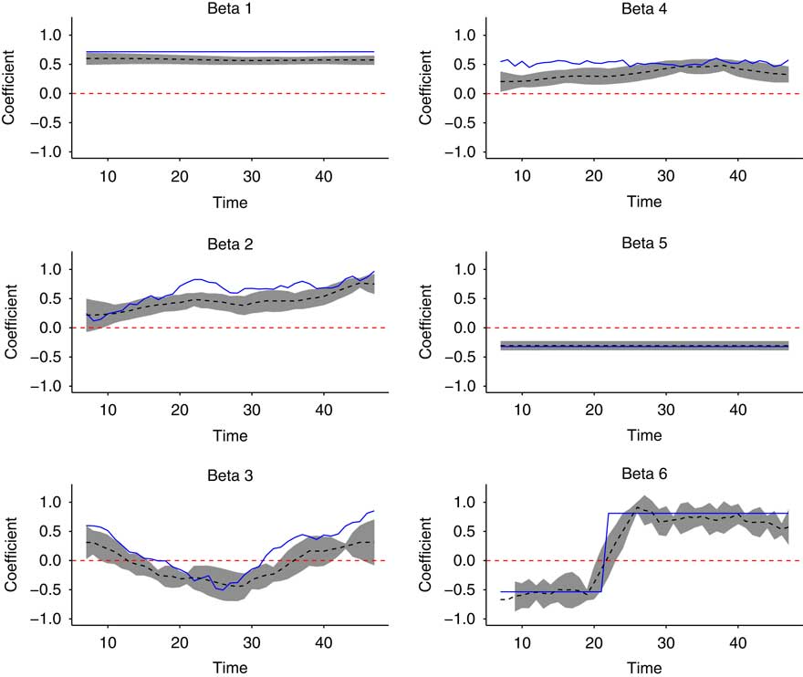
Figure 3 Estimated and true time-varying coefficients from simulated data. Note: The solid line is the known value of the coefficient. The dashed lines plot central predictions of dynamic effect coefficients, and the grey regions are 95% confidence intervals around those predictions.

The timing of these effect estimates is noteworthy. The most negative estimate falls in 1967, following the major escalation of US involvement in Vietnam after the Gulf of Tonkin Resolution, whereas the most positive estimate falls in 2004, as the depth of US involvement required in Iraq was becoming clear the year after declaring victory. At these times of major foreign escalations, the partisanship of the House of Representatives is likely most important to presidents’ ability to mobilise resources for increases in the defense budget. After all, the late 1960s and the early 2000s were both periods of increasing defense budgets to accommodate expanding conflicts and they were also periods in which the presidents could rely on copartisan majorities in the House. Such partisan dynamics are in line with recent qualitative, comparative studies (e.g. Mortensen et al. Reference Mortensen, Green-Pedersen, Breeman, Chaqus-Bonafont, Jennings, John, Palau and Timmermans2011), but have not gained much scholarly attention in time series analyses of public policy and public spending.

Fourth, the effect of the lagged national unemployment rate also merits attention. This effect estimate shows evidence of minor gradual changes in effect, going from a significant relationship to defense spending until the period of the Reagan buildup, after which it no longer shows a statistical relationship to changes in defense spending. Thus, our model indicates that the traditional expectation that increasing defense spending is a way to offset unemployment finds support throughout most of our time series up until the last year of the Reagan buildup. However, after this point, we no longer find a statistically significant relationship. This finding is a strong candidate for a case in which politicians’ core beliefs about policy have evolved. By the time of the defense buildup in the first part of the new century, several trends made defense spending a less useful tool for addressing unemployment: responding to international terrorism lent itself less to massive buildups of troops and bases, and sizable portions of defense spending were outsourced to private contracts. Thus, the logic underlying the former connection between unemployment and defense spending altered in the mid-1980s and seemingly has not returned.

Finally, public sentiment that defense is an important problem shows no association to defense spending changes, being consistently statistically insignificant and near zero. Likewise, presidential election years show no relationship to the outcome either.

DLM accuracy using simulated data

The model description demonstrates the DLM is capable of estimating coefficients that change with time, and our empirical examples show how these models can help us learn about policy-making trends. Nevertheless, it is another matter to ask whether the dynamic estimates from a DLM are necessarily the “true” coefficients we would like to recover from the estimation. We examine this latter, more crucial, question by simulating a time series of 41 observations on which to test our model. The chosen number of observations reflects the length of our actual time series used to generate Figure 1. We simulate a mix of six dynamic and constant true effect parameters and use them to calculate a simulated outcome variable that is a function of six randomly simulated explanatory variables and a normally distributed error term.

The design of the simulation reflects different types of time-varying relationships implied by policy theories. While the framework of punctuated equilibrium theory claims that changes can be sudden and quite dramatic, the advocacy coalition framework depicts more gradual changes, and a similar shape of change would be expected from the social learning perspective. In addition, it is important to validate that the DLM can in fact return constant effects where appropriate. Thus, two of the six factors are related to the outcome via constants (Beta 1 and Beta 5). One is constant except for a single large shift from a negative to a positive effect (Beta 6), which is chosen in order to examine whether the approach can pick up a major and sharp punctuation in the relationship between the explanatory variable and the outcome variable. One is related to the outcome via a coefficient that varies randomly according to a normal distribution over time but has no systematic pattern (Beta 4). Finally, two of these factors are related to the outcome via effect coefficients exhibiting distinct, gradual temporal patterns (Beta 2 and Beta 3).

The factors themselves, our simulated explanatory variables, are a matrix of six random vectors drawn from standard normal distributions. The outcome variable is calculated deterministically from the data and the true effects we wish to recover, after which we add a realisation of mean-zero normally distributed random noise to each observation. We exclude an intercept term from the model and, prior to running the model, we standardise the outcome by subtracting its mean and dividing by its standard deviation. We do not transform the explanatory variables, as they are random draws from standard normal distributions.

Figure 3 shows the results of running our DLM on this simulated data. The solid lines plot the true coefficients for our model and the dashed lines surrounded by grey confidence intervals plot our estimates of them. The model is quite successful at tracking how coefficients evolve over time, in the case of the two dynamic coefficients (Beta 2 and Beta 3), and it filters out noise to estimate Beta 4 as roughly constant. Beta 1 and Beta 5 are estimated accurately as constants, though the estimate for Beta 1 is biased slightly downward. Finally, the model converges to a roughly correct estimate of Beta 6, though it estimates the last few observations somewhat too conservatively.

We note that repeating this test with all coefficients varying dynamically, or none varying dynamically, does not substantively change the accuracy. Maintaining the same patterns of dynamics and the same number of independent variables, we can also demonstrate that changing the length of the time series has relatively little impact on model performance. We refer the reader to the Online Appendix G for graphs of these models in which we vary the length of the time series from a low of 30 observations to a high of 100 observations. Results are virtually identical to those reported here, though confidence intervals shrink with longer time series.

These are important evidence demonstrating that the DLM modelling approach is sensitive to various types of transformative changes, both the gradual movement predicted by the social learning and advocacy coalition framework, as well as the more punctuated changes of main interest to the punctuated equilibrium theory. It should be noted, however, that these findings do not amount to conclusive evidence that the DLM will recover the true coefficients under all circumstances, only that the DLM can recover true estimates under conditions similar to our own empirical tests. We encourage the reader to perform simulations emulating the patterns of variation in their own data when applying the DLM. To aid in this, we provide example code in the Online Appendix H for creating simulations like our own using the R statistical software environment and the “dlm” package (Petris Reference Petris2010).

Extending DLMs to panel data

Sometimes policy scholars utilise panel data, for instance, several countries observed over time, to evaluate dynamic policy theories. Extending DLMs using panel data can be accomplished in several ways. Two common choices are to model the panel time series in the DLM framework either as seemingly unrelated time series equations (SUTSE) or by using a hierarchical model with levels accommodating panel variation. In the former approach, the model structure is virtually the same as above except that errors in both the measurement and state equations are assumed correlated across panel units within time periods (Petris et al. Reference Petris, Petrone and Campagnoli2009, 132–134). This amounts to a partial relaxation of the assumption that all errors are independent. Errors in a SUTSE DLM model take a block diagonal form, in which errors within a period across units are correlated and all other errors are independent. It can, however, become computationally demanding to estimate the large covariance matrices that result when the number of panel units is large.

In such cases, an alternative is to estimate a dynamic hierarchical model. In this framework, the state equation has (at least) two levels. The dynamic coefficient estimates (in the measurement equation) are estimated as realisations from an underlying state (first state level), and the state varies as a Markov chain over time (second state level) (Petris et al. Reference Petris, Petrone and Campagnoli2009, 134–136). This introduces dependence across panel units, which also varies dynamically, without requiring estimation of large covariance matrices. In such a framework, with panel units denoted by j, a basic model would be:

$$\matrix{ {y_{{jt}} \,{\equals}\,{\mib X}_{{{\mib jt}}} \bibeta_{{{\mib jt}}} {\plus}v_{{jt}} ,} \hfill & {v_{t} \,\sim\,i.i.d.(0,\sigma _{{jt}}^{2} )} \hfill \vskip 10pt \cr {\bibeta_{{{\mib jt}}} \,{\equals}\, \bilambda _{{\mib t}} {\plus}{\epsilon}_{{{\mib jt}}} ,} \hfill & {{\epsilon}_{{{\mib jt}}} \,\sim\,i.i.d.(0,\Sigma _{t} )} \hfill \vskip 10pt\cr {\bilambda_{{\mib t}} \,{\equals}\, \bilambda_{{{\mib t}{\minus}{\bf 1}}} {\plus}{\mib w}_{{\mib t}} ,} \hfill & {{\mib w}_{{\mib t}} \,\sim\,i.i.d.(0,Q)} \hfill \cr } $$

It remains, as Commandeur et al. (Reference Commandeur, Koopman and Ooms2011) noted, that, at the time of writing, not all software packages for estimating DLMs support every form of DLM. Readers who find their preferred software does not include commands for easily estimating dynamic hierarchical or seemingly unrelated regressions can find this functionality in the “dlm” package for R. Similarly, readers who wish to estimate dynamic nonlinear regressions will find that, at the time of writing, “dlm” does not provide commands for this while MATLAB, RATS or the “KFAS” R package do provide such tools.